Multidimensional quantum cosmic models: New solutions and gravitational waves

Abstract

This paper contains a discussion on the quantum cosmic models, starting with the interpretation that all of the accelerating effects in the current universe are originated from the existence of a nonzero entropy of entanglement. In such a realm, we obtain new cosmic solutions for any arbitrary number of spatial dimensions, studying the stability of these solutions, so as the emergence of gravitational waves in the realm of the most general models.

I Introduction

No doubt, one of the greatest problems that the twenty-one century has inherited from the last decade of the twenty century and remains up today still unsolved is the so-called problem of the dark energy by which it appears to be completely impossible to account for the observed current accelerated expansion of the universe (which has been confirmed by several kinds of observational checking) by only using classical general relativity and its conventional cosmological solutions [1]. So far, two streams have been mostly followed to try to solve that problem by implementing the necessary cosmic repulsive force either by including a scalar field, called quintessence [2] or k-essence [3], or modifying the Hilbert-Einstein gravity action by adding suitable extra terms to it [4]. None of them appears to be consistent enough or could fulfill all observational requirements [5].

A theory which is self-consistent and agrees with all observational data has been recently proposed [6-9]. It is based on the assumption that all the accelerating effects come from the very quantum-entangled nature of the current universe [9,10]. In such a framework one can get essentially two relevant quantum solutions both of which can be seen as quantum perturbations to the de Sitter space [8,9], which is recovered in the classical limit where $\hbar\rightarrow 0$. It has been also shown that out from these two possible solutions only one of them satisfies the second law of thermodynamics [9], and hence is physically meaningful. It corresponds to a phantom universe [11] in that the parameter of the equation of state gets always on values which are less than -1, but does not show any violent instability [12] nor the sort of inconsistency coming from having a negative kinetic term for the scalar field - in fact, these models do not actually contain any scalar or other kinds of vacuum fields in their final equations. It is for these reasons that such a cosmic model has been also denoted as [8,9] benigner phantom model. On the other hand, given that de Sitter space is stable to scalar perturbations and that vectorial perturbations are in any case pure gauge [13], since the considered solutions can be regarded as nothing but scalar perturbations on de Sitter space, we ought to conclude that they are stable under such scalar harmonically symmetric perturbations and that those with vectorial character are also pure gauge in the case of the quantum solutions.

However, one cannot still be sure that the solution which has been chosen as the most physically relevant is stable under semiclassical and tensorial perturbations leading to gravitational waves. In this paper we shall study these two kinds of perturbations, showing that they in fact follows the same stability pattern as that of the de Sitter space. Our developments are made on a generalization of the quantum closed models to any number of dimensions and to the case in which a black hole is inserted in the space-time. Throughout this paper we will use natural unit so that $c=\hbar=1$, unless otherwise stated.

The paper can be outlined as follows. In Sec. II we very briefly review the quantum cosmic models, its origin and interpretation. The generalization of such models both to higher dimensions and to new models which contain a black hole are considered in Sec. III, together with a study of the static counterparts of such generalizations. Tensorial and semiclassical perturbations on the resulting closed cosmic models are studied in Sec. IV, briefly concluding in Sec. V.

II quantum cosmic models

As it was already advanced in the Introduction, the quantum cosmic models provide us with a dynamical cosmological scenario for the current evolution of the universe which uses just general relativity with or without a cosmological constant and the sharpest aspects of quantum mechanics, without inserting any kind of vacuum fields or introducing any extra terms in the Hilbert-Einstein gravitational action [6-9]. Such aspects can alternatively be viewed either as a sub-quantum potential or as due to the existence of an entanglement entropy for the currently accelerating universe. Because in Refs. [8] the first of these two equivalent interpretations was reviewed, we here summarize the main points of the quantum cosmic models by using also the second one. Actually, since the holographic version of the quantum cosmic models comes quite naturally from such models in terms of the physically consistent interpretation that the holographic screen coincides with the Hubble horizon [8], and at least one of the models (precisely that which satisfies the second law of thermodynamics) is formally equivalent with the Barrow’s hyper inflationary model [14], we shall now briefly comment on this interpretation.

Let us interpret from the onset the quantity $E_{Ent.}=a^{3}V_{SQ}$ as the total entanglement energy [10] of a universe with scale factor $a\equiv a(t)$ and whose matter-radiation content can be characterized by a sub-quantum potential density $V_{SQ}$ [6-9]. In such a case, the latter potential can simply be taken to describe the entanglement energy density of the universe, which we will denote as $\epsilon_{Ent.}\equiv E_{Ent.}/a^{3}$. In this way, because of the additiveness of the entanglement entropy, one can add up [15] the contributions from all existing individual fields in the observable universe in such a way that the entropy of entanglement $S_{Ent.}=\beta R_{H}^{2}$, with $\beta$ a constant that includes an account for the spin degrees of freedom of the quantum fields in the Hubble observable volume of radius $R_{H}$ and a numerical constant of order unity [15]. On the other hand, the presence of a boundary at the horizon leads us to conclude that the entanglement energy ought to be proportional to the radius of the associated spherical volume, that is $E_{nt.}=\alpha R_{H}$, with $\alpha$ a given constant, and hence again $S_{Ent.}=\beta R_{H}^{2}$.

It is worthy to notice that we can then take the temperature derived from the thermodynamics of the quantum cosmic model respecting the second law with $a=a_{+}$ as the entanglement temperature so that $T(a_{+})=E_{Ent.}/k_{B}$. Using now the general expression [10]

$$dE_{Ent.}=T_{Ent.}dS_{Ent.},$$

where $T_{Ent.}=(2\pi R_{H})^{-1}$ is the Hawking-Gibbons temperature, we consistently recover once again the expression $S_{Ent.}=\beta R_{H}^{2}$ for $\alpha=\beta/\pi$. That result is also consistent with the most natural holographic expression [8] $\rho=3/(8\pi GR_{H}^{2})$, described in terms of the Hubble horizon in the quantum cosmic models.

The models based on a sub-quantum potential and those derived from the existence of an entangled energy in the universe are all originated from the consideration of a Langrangian density given by [6-8]

$$L=V(\phi)\left[E(x,\kappa)-\sqrt{1-\dot{\phi}^{2}}\right],$$

where $\phi$ is an auxiliary scalar field, $V(\phi)=\tilde{V(\phi)}/a^{3}$ is its associated potential energy density, $E(x,\kappa)$ is the elliptic integral of the second kind, with $x=\arcsin\sqrt{1-\dot{\phi}^{2}}$ and $\kappa=\sqrt{1-V_{SQ}^{2}/v(\phi)}\equiv\sqrt{1-\epsilon_{Ent.}^{2}/V(\phi)}$, where $V_{SQ}=\tilde{V}_{SQ}/a^{3}$ is the sub-quantum potential density.

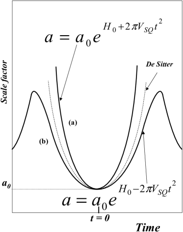
Figure 1: Cosmic solutions that result from the introduction of an energy density of entanglement $\epsilon_{Ent.}\equiv V_{SQ}$, where $V_{SQ}$ is the sub-quantum potential. Solution (a) goes like in De Sitter space with the same $H_{0}$, but with higher acceleration. Solution (b) corresponds to the case where $H_{0}^{2}>4\pi\epsilon_{Ent.}$ and represents a universe which is initially expanding in an accelerated way (at a rate slower than in De Sitter space with the same $H_{0}$), then expands in a decelerated way for a while to finally contract toward a zero radius as $t\rightarrow\infty$. On the figure we have used units such that $\hbar=c=G=1$

The above Lagrangian density vanishes in the classical limit $\hbar\rightarrow 0$. Adding physically reasonable regularity conditions for $\ddot{\phi}$ [7,8] we get $\dot{\phi}^{2}=1$. Thus, the use of the above Lagrangian density and the Lagrange equations, together with the final formulae derived in Ref. [8] then yield the following general expressions for the energy density and pressure

$$\rho=\frac{p}{w(t)}=6\pi G\left(\dot{H}^{-1}HV_{SQ}\right)^{2}\equiv 6\pi G\left(\dot{H}^{-1}H\epsilon_{Ent.}\right)^{2},$$ (1)

and for the time -dependent parameter of the equation of state $p=w(t)\rho$

$$w(t)=-\left(1+\frac{2\dot{H}}{3H^{2}}\right),$$ (2)

with

$$\dot{H}=\pm 4\pi GV_{SQ}\equiv\pm 4\pi G\epsilon_{Ent.}$$ (3)

$$H=\pm 4\pi GV_{SQ}t+H_{0}\equiv\pm 4\pi G\epsilon_{Ent.}t+H_{0},$$ (4)

and the set of cosmic solutions

$$a_{\pm}=a_{0}\exp\left(Ht\pm 2\pi GV_{SQ}t^{2}\right)\equiv a_{0}\exp\left(Ht\pm 2\pi G\epsilon_{Ent.}t^{2}\right).$$ (5)

In Eqs. (2.2)-(2.5) $H=\dot{a}/a$, $H_{0}$ is an integration constant playing the role of a cosmological term, $H_{0}=\Lambda^{1/2}$, and $a$ is the scale factor with $a_{0}$ its minimum value at time $t=0$. Eqs. (2.3) - (2.5) are valid only for sufficiently large $t$ or large $H_{0}$. From the set of solutions implied by Eq. (2.5) we shall disregard from the onset the one corresponding to $H_{0}=0$ and $t=\sqrt{\frac{\ln(a_{0}/a)}{2\pi GV_{SQ}}}$ as it would predict the unphysical case of a universe which necessarily is currently contracting. The chosen solutions are depicted in Fig.1 as compared to the usual flat de Sitter solution.

Actually, any account for the interpretation based on the cosmic entangled energy density $\epsilon_{Ent.}$ can straightforwardly be obtained from the corresponding account given in Refs. [6-9] given in terms of the sub-quantum potential, by simply replacing the sub-quantum potential energy density $V_{SQ}$ for $\epsilon_{Ent.}$ in all reasoning and formulae. Two points should be stressed now nevertheless. On the one hand, it is worth remarking that one would not expect $\tilde{V}_{SQ}$ to remain constant along the universal expansion, but to steadily increase like the volume of the universe $V=a^{3}$ does [8]. In order for obtaining the above relevant solutions one then must realize that it is the sub-quantum potential energy density $V_{SQ}=\tilde{V}_{SQ}/a^{3}$ appearing in the above Lagrangian density what should then be expected to remain constant at all cosmic times and, since we have consistently taken [8] $a^{3}V_{SQ}$ to be the total entanglement energy of the universe, the right-hand-side of solutions (2.5) appear to be correct, too. On the other hand, the scenarios we are considering are meant to evade or at least ameliorate he cosmic coincidence problem in the following sense. Whereas the sub-quantum potential density has to be chosen small enough to produce a sufficient late time domination, at the same time no problematic fine-tuning would be required for $\tilde{V}_{SQ}$ which must take on varying nearly arbitrary large values because of the very large values of the scale factor during the cosmic acceleration. In addition, since in the present scenarios all existing matter particles and fields should be associated with a sub-quantum potential (or entanglement entropy) and one can show [9] that that potential (or entangled energy) would make the effective mass of particles and field to vanish precisely at the coincidence time, then a cosmic system can be most naturally allowed where the matter dominance phase is followed by the accelerating expansion without any conceptual problem.

Current data based on a variety of observations [5] appear to point out to a present value for the parameter of the equation of state $w=-1$, with a bias toward slightly smaller values, that is to say, currently $w$ can possibly be less than -1 by a very small amount. This is actually the case that corresponds to the so called phantom energy [11], a form of dark energy which shows two main fundamental problems, a negative kinetic term in the Lagrangian and a fatal singularity in the finite future [11] which is associated with violent instabilities [12] and classical violation of the dominant energy condition. While solution $a_{+}$, (a) in Fig. 1, would approach the observational data as closely as we want, it does not show any of the problems which have been ascribed to phantom energy. Moreover, the given solution appears [8]: (i) to be stable, (ii) having suitable thermodynamic properties that consistently generalize those of the de Sitter space and (iii) entails a admissible residual quantum violation of the dominant energy condition ($\rho+p=-\epsilon$) leading to consistent quantum wormhole solutions; on the other hand, (iv) that description admits a most natural holographic extension where the holographic screen is placed at the Hubble horizon, and (v) it entails a perturbed metric which is no longer static but consistently reduces to static de Sitter metric in the limit where $w\rightarrow-1$ [8].

It it worth noticing finally that what actually matters in the models dealt with in this section is that some quantum-mechanical effects, which originally sub-dominated in the matter-dominated phase, eventually started driving cosmic acceleration.

III Generalized cosmic solutions

It has been already seen that the quantum cosmic solutions can be seen as either some generalizations from the flat version of de Sitter space or, if $V_{SQ}$ is sufficiently small, such as it appears to actually be the case, as perturbations of that de Sitter space. Since most of such models correspond to equations of state whose parameter is less than -1, such as it was mentioned before, they are also known as benigner phantom cosmic models [6-9]. In this section we shall derive even more general expressions for these quantum cosmic solutions by (i) considering the similar generalizations or perturbations of the hyperbolic version of the de Sitter space, and (ii) using a $d$-dimensional manifold. Actually, some observational data have implied that our universe is not perfectly flat and recent works [17,18] contemplate the possibility of the universe having spatial curvature. Thus, although WMAP alone abhors open models, requiring $\Omega_{total}\equiv\Omega_{m}+\Omega_{\Lambda}=1-\Omega_{k}\geq 0.9$ (95%), closed model with $\Omega_{total}$ as large as 1.4 are still marginally allowed provided that the Hubble parameter $h\sim 0.3$ and the age of the Universe $t_{0}\sim 20Gyr$. The combinations of the WMAP plus the SNIa data or the Hubble constant data also imply the possibility of the closed universe, giving curvature parameters $k=-0.011\pm 0.012$ and $k=-0.014\pm 0.017$, respectively [17], although the estimated values are still consistent with the flat FRW world model. Moreover, in Ref. [19] it is said that the best fit closed universe model has $\Omega_{m}=0.415$, $\Omega_{\Lambda}=0.630$ and $H_{0}=55kms^{-1}Mpc^{-1}$ and is a better fit to the WMAP data alone than the flat universe model $(\Delta\chi_{eff}^{2}=2$. However, the combination of WMAP data with either SNe data, large-scale structure data or measurements of $H_{0}$ favors models with $\Omega_{K}$ close to 0.

The $d$-dimensional de Sitter space has already been considered elsewhere [16]. Here we shall extend it to the also maximally symmetric space whose spacetime curvature is still negative (positive Ricci scalar) but no longer constant. Our spacetime will be solution of the Einstein equation

$$R_{ab}=t_{ab},\;\;a,b=0,1,...(d-1),$$ (6)

with

$$t_{ab}=\left(H\pm\hbar\xi t\right)^{2}g_{ab},$$ (7)

where $H^{2}=\Lambda/(d-1)$ is a cosmological constant and the constant $\hbar\xi$ generalizes the sub-quantum potential considered in the quantum cosmic models described in Sec. II. We notice that in the classical limit $\hbar\rightarrow 0$ the above definition becomes that of the usual $d$-dimensional de Sitter space. We shall restrict ourselves in this paper to the case in which our generalized $d$-dimensional de Sitter space can still be visualized as a $d+1$ hyperboloid defined as [20]

$$-x_{0}^{2}+\sum_{j=1}^{d}x_{j}^{2}=H^{-2}.$$ (8)

This $(d+1)$-dimensional hyperboloid is embedded in E^d+1, so that the most general expression of the metric for our extended quantum-corrected solutions is provided by the metric induced in this embedding, that is

$$ds^{2}=-dx_{0}^{2}+\sum_{j=1}^{d}dx_{j}^{2},$$ (9)

which has the same topology and invariance group as the $d$-dimensional de Sitter space [16].

This metric can now be exhibited in coordinates $\Theta_{\pm}=t(1\pm\hbar\xi t/H)\epsilon(\mp H_{0}/(4\hbar\xi),\pm\infty)$ (notice that our solutions then only covers a portion of the de Sitter time, while $t\epsilon(-\infty,+\infty)$), $\psi_{d-1},\psi_{d-2},...\psi_{2}\epsilon(0,\pi)$, $\psi_{1}\epsilon(0,2\pi)$, defined by

$$x_{d}=H^{-1}\cosh(H\Theta)\sin\psi_{d-1}\sin\psi_{d-2}...\sin\psi_{2}\cos\psi_{1}$$

$$x_{d-1}=H^{-1}\cosh(H\Theta)\sin\psi_{d-1}\sin\psi_{d-2}...\sin\psi_{2}\sin\psi_{1}$$

$$x_{d-2}=H^{-1}\cosh(H\Theta)\sin\psi_{d-1}\sin\psi_{d-2}...\cos\psi_{2}$$

(10)

$$x_{1}=H^{-1}\cosh(H\Theta)\cos\psi_{d-1}$$

$$x_{0}=H^{-1}\sinh(H\Theta),$$

which should be referred to as either time $\Theta_{+}$ or time $\Theta_{-}$. In terms of these coordinates metric (3.4) splits into

$$ds_{\pm}^{2}=-\left(1\pm\frac{2\hbar\xi t}{H}\right)^{2}dt^{2}$$

$$+H^{-2}\cosh^{2}\left[t\left(H\pm\hbar\xi t\right)\right]d\Omega_{d-1}^{2},$$ (11)

where $d\Omega_{d-1}^{2}$ is the metric on the $(d-1)$-sphere. Metric (3.6) is a closed $(d-1)$-dimensional Friedmann-Robertson-Walker metric whose spatial sections are $(d-1)$-spheres of radius $H^{-1}\cosh(H\Theta)$. The coordinates defined by Eqs. (3.5) describe two closed quantum cosmic spaces, $B_{\pm}$, which interconvert into each other at $t=0$. $B_{+}$ first steadily contracts until $t=0$ where it converts into $B_{-}$ to first expand up to a finite local maximum value at $t=H/(2\hbar\xi)$, then contract down to $a_{0}$ at $t=H/(\hbar\xi)$, expanding thereafter to infinite. $B_{-}$ would first contract until $t=-H/(\hbar\xi)$, then expand up to reach a local maximum at $t=-H/(2\hbar\xi)$, to contract again until $t=0$, where it converts into $a_{+}$ which will steadily expand thereafter to infinite.

In terms of the conformal times $\eta_{\pm}=\int d\Theta_{\pm}/a_{\pm}$, which is given by

$$\tan\eta_{\pm}=\sinh\left(t\pm\hbar\xi t^{2}/H\right),$$ (12)

with $\pi/2\geq\eta_{+}\geq 0$ and $3\pi/2\geq\eta_{-}\geq\pi$, the metrics can be re-expressed in a unitary form as

$$ds_{\pm}^{2}=\frac{a_{0}^{2}}{\cos^{2}\eta_{\pm}}\left(-d\eta_{\pm}^{2}+\gamma_{\alpha\beta}dx^{\alpha}dx^{\beta}\right),\alpha,\;\beta=1,2,...(d-1),$$ (13)

where $\gamma_{\alpha\beta}$ is the metric for a unit $(d-1)$-sphere.

We shall consider in what follows the equivalent in our quantum cosmic scenarios of the static ($d-1$)-dimensional metric. Let us use the new coordinates

$$x_{d}=H^{-1}\sin\psi_{d-1}\sin\psi_{d-2}...\sin\psi_{2}\cos\psi_{1}$$

$$x_{d-1}=H^{-1}\sin\psi_{d-1}\sin\psi_{d-2}...\sin\psi_{2}\sin\psi_{1}$$

$$x_{d-2}=H^{-1}\sin\psi_{d-1}\sin\psi_{d-2}...\cos\psi_{2}$$

(14)

$$x_{3}=H^{-1}\sin\psi_{d-1}\sin\psi_{d-2}cos\psi_{d-3}$$

$$x_{2}=H^{-1}\sin\psi_{d-1}\cos\psi_{d-2}$$

$$x_{0}=H^{-1}\cos\psi_{d-1}\sinh(H\Theta^{\prime})$$

which are defined by $t^{\prime}\epsilon(-\infty,+\infty)$), $r\epsilon(0,H^{-1})$, $\psi_{d-1},\psi_{d-2},...\psi_{2}\epsilon(0,\pi)$, $\psi_{1}\epsilon(0,2\pi)$. These coordinates will again be referred to either time $\Theta_{+}^{\prime}$ or time $\Theta_{-}^{\prime}$. Setting $r=H^{-1}\sin\psi_{d-1}$, we then find the metrics

$$ds_{\pm}^{2}=-\left(1\pm\frac{\hbar\xi t^{\prime}}{H}\right)^{2}dt^{\prime 2}\left(1-H^{2}r^{2}\right)$$

$$+\frac{dr^{2}}{1-H^{2}r^{2}}+r^{2}d\Omega_{d-2}^{2},$$ (15)

where $d\Omega_{d-2}^{2}$ is the metric on the $(d-2)$-sphere. We immediately note that this metric is no longer static. The coordinates defined by that metric cover only the portion of the spaces with $x_{1}>0$ and $\sum_{j=2}^{d}x_{j}^{2}<H^{-2}$ (?), i.e. the region inside the particle and event horizons of an observer moving along $r=0$.

Respective instantons can now be obtained by analytically continuing $\Theta_{\pm}\rightarrow i{\rm T}_{\pm}$ (where we have taken $\Theta^{\prime}\equiv\Theta$ for the sake of simplicity in the expressions), that is $t^{\prime}\rightarrow i\tau$ and $\xi\rightarrow-i\chi$, which contain singularities at $r=H^{-1}$, which are only apparent singularities if ${\rm T}_{\pm}$ are identified with periods $\pm 2\pi H^{-1}$, or in other words, if $\tau$ is respectively identified with periods $H(\sqrt{1+8\pi\hbar\chi H^{-2}}\pm 1)/(2\hbar\chi)$. It follows then that the two spaces under consideration would respectively behave as though if they would emit a bath of thermal radiation at the intrinsic temperatures given by

$$T_{\pm}^{th}=\frac{2\hbar\chi}{H\left(\sqrt{1+8\pi\hbar\chi H^{-2}}\pm 1\right)}.$$ (16)

It must be remarked that in the limit when $\chi\rightarrow 0$, both temperatures $T_{\pm}^{th}$ consistently reduce to the unique value $H/(2\pi)=\sqrt{\Lambda(d-1)^{-1}}/(2\pi)$, that is the temperature of a $d$-dimensional de Sitter space [16], even though $T_{-}^{th}$ does it more rapidly than $T_{+}^{th}$ (in fact, for sufficiently small $\chi$, we can check that $T_{-}^{th}\simeq H/(2\pi)$ and $T_{+}^{th}\simeq\hbar\chi H/(H^{2}+2\pi\hbar\chi)$). Note that while we keep $\hbar$ in all definitions concerning the quantum cosmic spaces, natural units so that $\hbar=G=c=k_{B}=1$ are otherwise used when such definitions are used. Now, one can estimate the entropy of these spaces by taking the inverse to their temperature. Thus, it can be seen that the entropy of the universe with scale factor $a_{+}$ will always be larger than that for a universe with scale factor $a_{-}$. It follows then that whereas the transition from $a_{+}$ to $a_{-}$ at $t=0$ would violate the second law of thermodynamics, the transition from $a_{-}$ to $a_{+}$ at $t=0$ would satisfy it, so making the model with scale factor $a_{+}$ evolving along positive time more likely to happen.

The time variables $t$ and $t^{\prime}$ in Eqns. (3.2), (3.5) and (3.9) do not admit any bounds other than ($-\infty$, $+\infty$), so that the involved models can be related with the Barrow’s hyper inflationary model [14], albait the solution $a_{+}$ here always respect the second law of thermodynamics because for such a solution the entropy is an ever increasing function of time [8].

Before closing up this section we shall briefly consider the static Schwarzschild-quantum mechanically perturbed solutions. It can be shown that in that case the line element is again not properly static as they depend on time in their $g_{tt}$ component, that is

$$ds_{\pm}^{2}=-\left(1\pm\frac{\hbar\xi t^{\prime}}{H}\right)^{2}dt^{\prime 2}\left(1-\frac{2M}{r}-H^{2}r^{2}\right)$$

$$+\frac{dr^{2}}{1-\frac{2M}{r}-H^{2}r^{2}}+r^{2}d\Omega_{d-2}^{2},$$ (17)

Instantons for such solutions can also be similarly constructed. One readily may show that again such instantons describe thermal baths at given temperatures given now by

$$T_{\pm}^{th}=\frac{2\hbar\chi}{H\left(\sqrt{1+8\pi\hbar\chi H^{-2}}\pm 1\right)\left(1\mp\frac{2}{3}\epsilon\right)+O\left(\epsilon^{2}\right)}.$$ (18)

where the second sign ambiguity in the denominator refers to the cosmological (upper) and black hole (lower) horizons and, according to Ginsparg and Perry [13], $9M^{2}\Lambda=1-3\epsilon^{2}$, with $0\leq\epsilon<<1$, the degenerate case corresponding just to $\epsilon\rightarrow 0$.

IV Gravitational waves and semiclassical instability

In this section we shall restrict ourselves to the solutions derived in the previous section for just the four-dimensional case, considering the generation of gravitational waves in the realm of such solutions and some semiclassical instabilities that arise when one Euclideanizes ($t\rightarrow i\tau$) the higher-dimensional solutions. Thus, let us consider first the tensorial Liftshif-Khalatnikov perturbations corresponding to the zeroth mode $\ell=0$. From them we can derive [13,16] the differential equation

$$\nu^{\prime\prime}+2\tan\eta\nu^{\prime}=0,$$ (19)

where $\eta$ and ${}^{\prime}=d/d\eta$ refer to the conformal time, either $\eta_{+}$ or $\eta_{-}$, defined in Eq. (3.7). This differential equation has as general solution

$$\nu=C_{0}+C_{1}\left(\eta+\frac{1}{2}\sin(2\eta)\right),$$ (20)

where $C_{0}$ and $C_{1}$ are given integration constants. We must now particularize solution (4.2) to be referred to $\eta_{\pm}$. In the case $\eta_{+}$ we see that the conformal time runs from $0$ ($t=0$) to $\pi/2$ ($t=\infty$). These waves do not destabilize the space as, though their amplitude does not vanish at the limit where $\eta_{+}\rightarrow\pi/2$, neither it grows with time $t$. For $\eta_{-}$ the conformal time runs from $\pi$ ($t=0$ or $t=H^{2}/(\hbar\xi)$) to $3\pi/2$ ($t=\infty$). It can be easily seen that neither these waves can destabilize the space.

For the general case $\ell\neq 0$, we have the general differential equation, likewise referred to either $\eta_{+}$ or $\eta_{-}$,

$$\nu^{\prime\prime}+2\tan\eta\nu^{\prime}+\ell(\ell+2)\nu=0.$$ (21)

The solution to this differential equation can be expressed as

$$\nu=\cos^{3}\eta C_{\ell-1}^{(2)}(\sin\eta),$$ (22)

with $C_{n}^{(\alpha)}$ the ultraspherical (Gegenbauer) polynomials of degree 2. Now, for $\eta_{+}=0$ or $\eta_{-}=\pi$, the amplitude vanishes for even $\ell=2,4,6,...$, and becomes

$$\nu=(-1)^{(\ell-1)/2}\frac{\Gamma\left(2+\frac{\ell-1}{2}\right)}{\Gamma(2)\left(\frac{\ell-1}{2}\right)!},$$

for odd $\ell=1,3,5,...$. For $\eta_{+}=\pi/2$, $\nu=(\ell+2)!/[6(l-1)!]$ and for $\eta_{-}=3\pi/2$, $\nu=(-1)^{\ell-1}(\ell+2)!/[6(l-1)!]$. Once again the considered spaces are therefore stable to tensorial perturbations for nonzero $\ell$. It is worth mentioning that for the solution corresponding to $\eta_{-}$ and even $\ell$, the absolute value of the amplitude of the gravitational waves would first increase from zero (at $t=0$) to reach a maximum value at $t=H/(2\hbar\xi)$, to then decrease down to zero at $t=H/(\hbar\xi)$, and finally steadily increase all the time to reach its final finite value of unit order as $t\rightarrow\infty$. Clearly. a distinctive observational effect predicted by that cosmic model would be the generation of gravitational waves whose amplitude adjusted to the given pattern.

A general derivation of Eqns. (4.1) and (4.3) from a general traceless rank-two tensor harmonics which is an eigenfunction of the Laplace operator on $S^{3}$ and satisfies the eigenvalue equation $\nabla_{a}\nabla^{a}H_{cd}^{(n)}=-(n^{2}-3)H_{cd}^{(n)}$ can be found in Refs. [13,16].

We add finally some comments to the possibility that our closed spaces develop a semiclassical instability. We shall use the Euclidean approach. In order to see if our Euclideanized solutions are stable or correspond to semiclassical instabilities, it will suffice to determine the eigenvalues of the differential operator [13,21]

$$G_{abcd}\Phi^{ab}\simeq-\Box\Phi_{cd}-2R_{acbd}\Phi^{ab}\simeq\lambda\Phi_{cd},$$ (23)

where $\Phi_{ab}$ is a metric perturbation. Now, if all $\lambda\geq 0$, the Euclideanized spaces are stable, showing a semiclassical instability otherwise. Stability can most readily be shown if, by analytically continuing metrics (3.10), the metric on the ($d-2$)-sphere, $d\Omega_{d-2}$, turns out to be expressible as the Kahler metric associated to a 2-sphere. Thus, let us introduce the complex transformation

$$Z=2\tan\left(\psi_{d-2}/2\right)\exp\left(i\int d\Omega_{d-3}\right),$$ (24)

and hence in fact we can derive

$$d\Omega_{d-2}=\frac{d\bar{Z}dZ}{\left(1+\frac{1}{4}\bar{Z}Z\right)^{2}}$$ (25)

and the Kahler potential

$$K=2\log\left(1+\frac{1}{4}\bar{Z}Z\right),$$ (26)

so showing that, quite similarly to what it happens in the $d$-dimensional de Sitter space, the instantons constructed from metrics (3.10) are stable. Whether or not a space-time corresponding to Schwarzschild-generalized de Sitter metric would show a semiclassical instability is a question that required further developments and calculations.

V conclusions and comments

This paper deals with new four-dimensional and $d$-dimensional cosmological models describing an accelerating universe in the spatially flat and closed cases. The ingredients used for constructing these solutions are minimal as they only specify a cosmic relativistic field described by just Hilbert-Einstein gravity and the notion of the quantum entanglement of the universe, that is the probabilistic quantum effects associated with the general matter content existing in the universe or its generalization for the closed cases. Two of such models correspond to an equation of state $p=w\rho$ with parameter $w<-1$ for their entire evolution, and still other of them which covers a period in its future also with $w<-1$; that is to say, these three solutions are associated with the so-called phantom sector, showing however a future evolution of the universe which is free from most of the problems confronted by usual phantom scenarios; namely, violent instabilities, future singularities, incompatibility with the previous existence of a matter-dominated phase, classical violations of energy conditions or inadequacy of the holographic description. Therefore we also denote such quantum cosmic models as benigner phantom models. All these models can be regarded as generalizations or perturbations of the either exponential or hyperbolic form of the de Sitter space. The hyperbolic solution are given in a $d$-dimensional manifold which is particularized in the four-dimensional case in the Euclideanized extension that allowed us to derive quantum formulas for the temperature that reduce to that of Gibbons-Hawking when the perturbation is made to vanish. Finally, the generation of gravitational waves in some of the considered models has been studied in the realm of the Lifshitz-Khalatnikov perturbation formalism for the spatially closed case. It is also shown that none of these waves destabilize the space-time, as neither the vector and scalar cosmological perturbations do in the spatially flat and closed cases.

- (1) T. Padmanabhan, Dark Energy: The Mystery of the Millennium, AIP Conf. Proc. 861: 179 - 196, 2006;1. P. de Bernardis et al., Nature 404, 955 2000); A. Balbi et al., Astrophys.J., 545, L1 (2000); S. Hanany et al., Ap.J., 545, L5 (2000); T.J. Pearson et al., Astrophys.J., 591, 556 (2003); C.L. Bennett et al, Astrophys. J. Suppl. ,148, 1 (2003); D. N. Spergel et al., Astrophys.J. Suppl. 148, 175 (2003); B. S. Mason et al., Astrophys. J. ,591, 540 (2003).
- (2) R.R. Caldwell, R. Dave and P.J. Steinhardt, Phys, Rev. Lett. 80, 1582 (1998); L. Wang and P.J. Steinhardt, Astrophys. J. 508, 483 (1998); R.R. Caldwell and P.J. Steinhardt, Phys. Rev. D57, 6057 (1998); P.F. González-Díaz, Phys. Rev. D62, 023513 (2000); I. Zlatev, L. Wang and P.J. Steinhardt, Phys. Rev. Lett. 82, 896 (1999); P.J. Steinhardt, L. Wang and I. Zlatev, Phys. Rev. D59, 123504 (1999); I. Zlatev and P.J. Steinhardt, Phys. Lett. B459, 570 (1999); P. Brax, J. Martin and A. Riazuelo, Phys. Rev. D62, 103505 (2000).
- (3) C. Armendáriz-Picón, T. Damour and V. Mukhanov, Phys. Lett. B458, 209 1999); J. Garriga and V. Mukhanov, Phys. Lett. B458, 219 (1999); T. Chiba, T. Okabe and M. Yamaguchi, Phys. Rev. D62, 023511 (2000); C. Amendáriz-Picón, V. Mukhanov and P.J. Steinhardt, Phys. Rev. Lett. 85, 4438 (2000); C. Amend ariz- 9 Pic on, V. Mukhanov and P.J. Steinhardt, Phys. Rev. D63, 103510 (2001) .
- (4) See e.g. E. Elizalde , S.Nojiri, S.D. Odintsov , D. Saez, V. Faraoni, Phys.Rev.D77:106005,2008.
- (5) D. J. Mortlock and R. L. Webster, Mon. Not. Roy. Astron. Soc. 319, 872 (2000) [arXiv:astro-ph/0008081]; A. G. Riess et al. [Supernova Search Team Collaboration], Astron. J. 116, 1009 (1998) [arXiv:astro-ph/9805201]; S. Perlmutter et al. [Supernova Cosmology Project Collaboration], Astrophys. J. 517, 565 (1999) [arXiv:astro-ph/9812133]; J. L. Tonry et al. [Supernova Search Team Collaboration], Astrophys. J. 594, 1 (2003); D. N. Spergel et al. [WMAP Collaboration], Astrophys. J. Suppl. 148, 175 (2003); C. L. Bennett et al., Astrophys. J. Suppl. 148, 1 (2003); M. Tegmark et al. [SDSS Collaboration], Phys. Rev. D 69, 103501 (2004).
- (6) P.F. González-Díaz, Dark energy without dark energy, AIP Conf. Proc. 878 (2006)
- (7) P.F. González-Díaz and A. Rozas-Fernández, Phys.Lett. B641, 134(2006).
- (8) P.F. González-Díaz and A. Rozas-Fernández, Class. Quant. Grav. 25, 175023 (2008).
- (9) P.F. González-Díaz and A. Rozas-Fernández, On the onset of the dark energy era, in: The Problems of Modern Cosmology, edited by P.M. Levrov (Toms State Univ. Press, Toms, Russia, 2009), pp. 202, e-Print: arXiv:0811.2948 [gr-qc] .
- (10) J.-W. Lee, J. Lee and H.-Chan Kim, JCAP 0708 (2007) 005; Quantum informational dark energy: Dark energy from forgetting, hep-th/0709.0047 .
- (11) R.R. Caldwell, Phys. Lett. B545, 23 (2002) .
- (12) S.M. Carroll, M. Hoffman and M. Trodden, Phys. Rev. D68, 023509 (2003).
- (13) P. Ginsparg and M.J. Perry, Nucl. Phys. B222, 245 (1983).
- (14) J.D. Barrow, Phys. Lett. B180 (1986) 335; B193 (1987) 285 .
- (15) S. Mukohyama, M. Seriu and H. Kodama, Phys. Rev. D55 (1997) 7666 .
- (16) P.F. González-Díaz, Phys. Rev. D36, 3651 (1987).
- (17) [1] C. L. Bennet et al., Astrophys. J. Suppl. 148, 1 (2003); D. N. Spergel, Astrophys. J. Suppl. 148, 175, (2003).
- (18) M. Tegmark et al. Phys.Rev.D69, 103501 (2004).
- (19) D.N. Spergel et al., Astrophys. J. Suppl. Ser. 170, 377 (2007).
- (20) E. Schrödinger, Expanding universe (Cambridge University Press, Cambridge, UK, 1965).
- (21) P.F. González-Díaz, Phys. Lett. B191, 263 (1987).