Origin of negative differential thermal resistance in nonlinear systems

Abstract

Negative differential resistance in electronic conduction has been extensively studied, but it is not the case for its thermal counterpart, namely, negative differential thermal resistance (NDTR). We present a classical Landauer formula in which the nonlinearity is incorporated by the self-consistent phonon theory in order to study the heat flux across a chain consisting of two weakly coupled lattices. Two typical nonlinear models of hard and soft on-site potentials are discussed respectively. It is shown that the nonlinearity has strong impacts on the occurring of NDTR. As a result, a transition from the absence to the presence of NDTR is observed. The origin of NDTR consists in the competition between the temperature difference, which acts as an external field, and the temperature dependent thermal boundary conductance. Finally, the onset of the transition is clearly illustrated for this model. Our analytical calculation agrees reasonably well with numerical simulations.

I Introduction

In the linear response regime, transport processes such as transport of mass, momentum or energy can be described by linear laws of the form

$$j=\mu F,$$ (1)

where $j$ and $F$ stand for the generalized flux and force, respectively, and $\mu$ the transport coefficient. In other words, the flux $j$ is a linearly increasing function of the external field $F$, which is a well-known characteristic of Fick’s law for mass transport, Ohm’s law for electron transport and Fourier’s law for heat transport. As the field $F$ becomes too strong, the system may come into the nonlinear response regime, where the linear relation (1) is no longer valid since the transport coefficient $\mu$ becomes itself field dependent. As a result, an interesting phenomenon, i.e. negative differential resistance (NDR) may take place in a system in the strong-field regime where the flux counter-intuitively decreases as the external field increases.

Since the pioneering observation in the tunnel diode by Esaki Esaki (1958), NDR has been extensively studied for the electronic transport, which led to widespread practical applications in modern electronics Sze and NG (2007). It is still an active research topic to date, particularly at the atomic scale Tu et al. (2008); Pati et al. (2008). However, its counterpart in the heat conduction problem, namely the negative differential thermal resistance (NDTR) has been much less studied. NDTR effect has been noticed in the studies of asymmetric heat conduction (see Fig. 1 in Refs. Li et al. (2004) and Hu et al. (2006)), where it has been shown to be critical to design a thermal diode with an enormous rectification factor. It has also been shown that NDTR is crucial for a correct functioning of lattice models of thermal transistor Li et al. (2006) and thermal logic gates Wang and Li (2007). It is already known that NDTR effect can be qualitatively explained in terms of the overlapping of the vibrational spectra of the interfacial particles Li et al. (2006); Wang and Li (2007). On the other hand, is has been recently shown that in the model presented in Li et al. (2006), the NDTR effect will gradually disappear as the system size increases or the properties of the interfacial coupling change Shao et al. (2009); Zhong et al. (2009). For a clear understanding of the mechanism underlying NDTR effect, it is thus imperative to comprehend from a quantitative point of view the necessary conditions for the occurring of NDTR effect.

As far as we know, a rigorous analytical approach to study heat conduction in a non-integrable lattice system at the nonlinear response regime has been so far unavailable. One usually has to rely on numerical simulations. In the present study, we will develop a phenomenological approach, in line with that in Ref. Hu et al. (2006), to study heat flux through an “interface” between two weakly coupled anharmonic segments. We study two typical models, which have hard and soft anharmonicity respectively. The theoretical calculation based on the presented Landauer-like formula yields results in reasonable agreement with the numerical simulation. We will show that the intrinsic nonlinearity of the system is necessary for the occurring of NDTR. It is further illustrated that NDTR does not always occur in the presence of nonlinearity. A transition from the absence to the presence of NDTR with the increase of the nonlinearity is illustrated for both models. A simple but physically appealing mechanism is proposed in order to explain the origin of NDTR in the nonlinear systems. Our study of NDTR provides indications of possible applications such as the construction of thermal devices.

II Theoretical approach

We study in this work the stationary heat current across a chain consisting of two weakly coupled lattices,

$$H=H_{+}+\frac{K_{int}}{2}(x_{1}-x_{0})^{2}+H_{-},$$ (2)

where the Hamiltonian for the left and right segments are given by

$$H_{+}=\sum^{0}_{i=-N/2+1}\frac{p_{i}^{2}}{2}+\frac{1}{2}(x_{i+1}-x_{i})^{2}+U_{+}(x_{i})$$ (3)

and

$$H_{-}=\sum^{N/2}_{i=1}\frac{p_{i}^{2}}{2}+\frac{1}{2}(x_{i+1}-x_{i})^{2}+U_{-}(x_{i}),$$ (4)

respectively. $U_{\pm}(x)$ represent the onsite potential that will be specified below. Two heat baths with temperatures $T_{+}$ and $T_{-}$ are connected to the extremities of the left and right segment, respectively. Note that NDTR effect have been so far investigated only in spatially asymmetric models Li et al. (2004); Hu et al. (2006); Li et al. (2006); Wang and Li (2007); Shao et al. (2009); Zhong et al. (2009). However, we will show in this study that NDTR can also take place in a spatially symmetric model, i.e. for $U_{+}(x)=U_{-}(x)$.

In the case where the coupling $K_{int}$ between the left and right segments is weak, the two segments will achieve two nearly equilibrium states at temperatures $T_{+}$ and $T_{-}$, respectively. Their vibrational motion can thus be approximately described according to the self-consistent phonon theory (SCPT) Brüesch (1982); Dauxois et al. (1993); Hu et al. (2006); He et al. (2008) with effective harmonic Hamiltonians $H_{+}^{(0)}$ and $H_{-}^{(0)}$ of the form

$$H_{+}^{(0)}=\sum^{0}_{i=-N/2+1}\frac{p_{i}^{2}}{2}+\frac{1}{2}(u_{i+1}-u_{i})^{2}+\frac{f_{+}}{2}u_{i}^{2},$$ (5)

$$H_{-}^{(0)}=\sum^{N/2}_{i=1}\frac{p_{i}^{2}}{2}+\frac{1}{2}(u_{i+1}-u_{i})^{2}+\frac{f_{-}}{2}u_{i}^{2},$$ (6)

with $u_{i}=x_{i}-\langle x_{i}\rangle=x_{i}-\eta$. The effective force constants $f_{\pm}$ are determined by numerically solving the self-consistent equations

$$f_{\pm}=2\frac{\partial\langle U_{\pm}(x)\rangle_{\pm}^{(0)}}{\partial\langle x^{2}\rangle_{\pm}^{(0)}}$$ (7)

Here $\langle...\rangle_{\pm}^{(0)}$ denotes the thermal average with respect to the trial harmonic Hamiltonian $H_{\pm}^{(0)}$ at the corresponding temperature $T_{\pm}$ and it is defined by

$$\langle A(\mathbf{u})\rangle_{\pm}^{(0)}=\frac{\int{A(\mathbf{u})\exp{(-\beta_{\pm}H_{\pm}^{(0)}(\mathbf{u}))}}\,\mathrm{d}\mathbf{u}}{\int{\exp{(-\beta_{\pm}H_{\pm}^{(0)}(\mathbf{u}))}}\,\mathrm{d}\mathbf{u}},$$ (8)

for a given measurable $A(\mathbf{u})$, where $\beta_{\pm}=(k_{B}T_{\pm})^{-1}$. Note that according to Eq. (8), $f_{\pm}$ is temperature dependent. The derivation of Eq. (7) can be found in the appendix of Ref. He et al. (2008). The renormalized normal-mode frequencies of phonons in each segment can then be written as $\omega_{\pm}(q)=\sqrt{4\sin^{2}{(q/2)}+f_{\pm}}$, where $q$ stands for the wave vector.

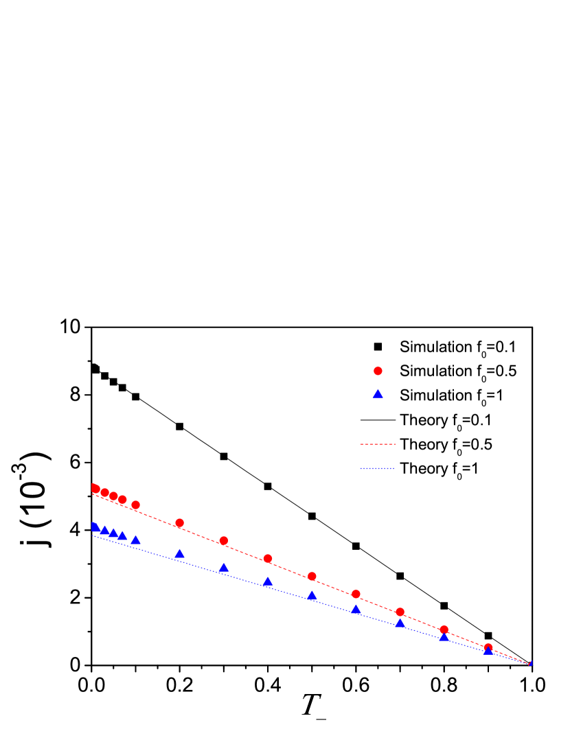
Figure 1: Heat flux $j$ as a function of $T_{-}$ for the symmetric harmonic chain ($\lambda=0,f_{L0}=f_{R0}=f_{0}$). Here $K_{int}=0.05$, $T_{+}=1$. The system size is $N=64$ for the simulation. The linear dependence of $j$ on $T_{-}$ implies that the transmission is temperature independent.

According to the Khalatnikov theory Khalatnikov (1965), the heat flux can be regarded as the propagation of plane waves (phonons) with various frequencies. Within this approach, the heat flux through the system composed of the segments  (5) and (6) can be determined by He (2008)

$$j=\frac{k_{B}(T_{+}-T_{-})}{2\pi}\int_{\omega_{min}}^{\omega_{max}}\mathcal{T}(\omega)\,\mathrm{d}\omega,\\$$ (9)

where $\omega_{min}$ and $\omega_{max}$ correspond to the boundaries of the overlap band of left and right phonon spectra, that is $\omega_{min}=\max\left\{\sqrt{f_{+}},\sqrt{f_{-}}\right\}$ and $\omega_{max}=\min\left\{\sqrt{4+f_{+}},\sqrt{4+f_{-}}\right\}$. $\mathcal{T}(\omega)$ is the phonon transmission probability through the interface. It is worth mentioning that Eq. (9) is similar in form to the celebrated Landauer formula

$$j=\frac{1}{2\pi}\int\mathcal{T}(\omega)[\eta_{+}(\omega,T_{+})-\eta_{-}(\omega,T_{-})]\hbar\omega\,\mathrm{d}\omega,$$ (10)

where $\eta_{\pm}=(e^{\beta_{\pm}\hbar\omega}-1)^{-1}$ are the Bose-Einstein distribution functions. The Landauer formula (10), originated from the study of electron transport Landauer (1957), describes the ballistic transport of phonons in quantum systems Rego and Kirczenow (1998). Considering the high temperature limit (classical limit) where $\eta_{\pm}\cong(\beta_{\pm}\hbar\omega)^{-1}$, Eq. (10) reduces to Eq. (9). Note that the quantum constant $\hbar$ is cancelled automatically in the classical limit. Thus our equation  (9) can be considered as the classical form of the traditional Landauer formula.

To find the transmission coefficient, we consider a plane wave incident from the left, which is partly reflected by the interface with amplitude $\bar{R}$ and partly transmits across the interface with amplitude $\bar{T}$ into the right segment Hu et al. (2006). The displacement of the $i$th particle from the equilibrium position can be written as

$$u_{i}=\begin{cases}(e^{Iki}+\bar{R}e^{-Iki})e^{-I\omega_{+}t},&\text{if $i\leq 0$}\\ \bar{T}e^{Iq(i-1)-I\omega_{-}t},&\text{if $i\geq 1$}\end{cases}$$ (11)

where $I$ is the imaginary unit. Thus the motion of the interface particles can be described by the following equations

$$-\omega_{+}^{2}u_{0} =u_{-1}+K_{int}u_{1}-(1+K_{int}+f_{+})u_{0},$$ (12a)

$$-\omega_{-}^{2}u_{1} =u_{2}+K_{int}u_{0}-(1+K_{int}+f_{-})u_{1}.$$ (12b)

If an acoustic matching condition $\omega_{+}=\omega_{-}=\omega$ is satisfied, the solution of Eq. (12) gives the transmission probability of Eq. (9) in the form

$$\mathcal{T}(\ \omega,f_{+}(T_{+}),f_{-}(T_{-})\ )=1-|\bar{R}^{2}|$$ (13)

$$=\frac{C_{2}K_{int}^{2}}{C_{1}(1-2K_{int})+C_{3}K_{int}^{2}},$$

where

$$C_{1}(\omega) =(\omega^{2}-f_{+})(\omega^{2}-f_{-})\hskip 1.42262pt,$$ (14a)

$$C_{2}(\omega) =\sqrt{C_{1}(4+f_{+}-\omega^{2})(4+f_{-}-\omega^{2})}\hskip 1.42262pt,$$ (14b)

$$C_{3}(\omega) =(C_{1}+C_{2})/2+2\omega^{2}-f_{+}-f_{-}\hskip 1.42262pt.$$ (14c)

Thermal transport is inhibited, i.e. $\mathcal{T}=0$ if the phonon bands of the two segments are mismatched.

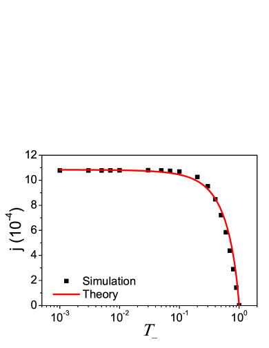
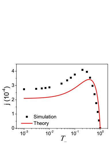
Figure 2: Heat flux $j$ as a function of $T_{-}$ for the $\phi^{4}$ model. Left: $\lambda=0.8$; Right: $\lambda=5$. In both cases, $K_{int}=0.05$, $T_{+}=1$ and $N=64$ for the numerical simulation.

In what follows, we will illustrate the results of the analytical calculation based on Eq. (9). As a comparison, non-equilibrium molecular dynamics (NEMD) simulations are performed by applying Langevin heat baths at the two extremities of the chain. The heat flux, whose definition can be found in Ref. Lepri et al. (2003), is averaged over a long enough time so that the system reaches the steady state regime, at which the local heat flux is constant along the chain. During the simulations, $T_{+}$ was fixed and the temperature difference $\Delta T=T_{+}-T_{-}$ was changed by changing $T_{-}$.

II.1 $\phi^{4}$ model

Let us first consider the $\phi^{4}$ model, which is a typical bounding potential of “hard” anharmonicity ,

$$U_{\pm}(x)=\frac{f_{0}}{2}x^{2}+\frac{\lambda}{4}x^{4}.$$ (15)

The effective force constants $f_{\pm}$ are determined by numerically solving the self-consistent equations

$$f_{\pm}=f_{0}+\frac{3\lambda k_{B}T_{\pm}}{\sqrt{f_{\pm}^{2}+4f_{\pm}}}.$$ (16)

Note that $f_{\pm}$ regularly increases with increasing temperature.

Before discussing the nonlinearity effect, we will apply the above analytical analysis to the harmonic model $\lambda=0$. In this case, the transmission (13) is temperature independent since $f_{\pm}=f_{0}$. Fig. 1 illustrates the heat flux $j$ as a function of $T_{-}$ for the harmonic chain for several values of the harmonic constant $f_{0}$. By inspecting the figure, we first notice that in the ballistic case, the simulation agrees well with the analytical result that follows from the classical Landauer formula (9) ($k_{B}=1$). Furthermore, it is seen that $j$ increases linearly when $T_{-}$ decreases, that is when the temperature difference increases. As is expected, NDTR cannot be observed in the harmonic model since there does not exist any nonlinear response mechanism.

Figure 3: $\phi^{4}$ model: The turning point $T^{*}$, at which the heat current exhibits a maximum, as a function of $\lambda$. Nonzero $T^{*}$ indicates the presence of NDTR. The transition from the absence to the presence of NDTR occurs at $\lambda_{c}\approx 1$.

Furthermore, Fig. 2 shows that if the nonlinearity is present inside each segment ($\lambda\neq 0$), the formula (9) still works reasonably well. By comparing the left and right plots of Fig. 2, it is seen that a transition from the absence to the presence of NDTR occurs as the nonlinearity $\lambda$ increases. We also present in Fig. 3 the evolution of the turning point $T^{*}$ at which NDTR effect manifests itself as a function of the nonlinearity. The on-set of NDTR at $\lambda_{c}\approx 1$ is clearly shown.

Note that Eqs. (16) and (9) implies the following scaling relation

$$j(T_{\pm},\lambda)=sj(T_{\pm}/s,s\lambda),$$ (17)

where $s$ is an arbitrary scaling constant. The same scaling property can be obtained from the equations of motion of the model (2)(see Dhar (2008)). Eq. (17) indicates the equivalence between the temperature and the nonlinearity. Thus a similar transition for fixed $\lambda$ can be observed as $T_{+}$ increases, which will be verified both from numerical simulations and our analytical approach. In fact, NDTR takes place if $\lambda>\lambda_{c}$ (or $T_{+}>T_{c}$).

II.2 On-site Morse model

Now we consider a model which consists of two weakly coupled symmetric nonlinear lattices with an on-site Morse potential given by

$$U_{\pm}(x)=D[\,\exp{(-\alpha x)}-1]^{2}.$$ (18)

Model (18) was introduced in order to investigate the DNA denaturation process Peyrard and Bishop (1989). The anharmonicity of the model is “soft” since the Morse potential is bounded for $x\rightarrow\infty$.

The effective force constants $f_{\pm}$ are obtained by numerically solving the following self-consistent equations

$$f_{\pm}=2\alpha^{2}D\exp{\left(-\frac{\alpha^{2}k_{B}T_{\pm}}{\sqrt{f_{\pm}^{2}+4f_{\pm}}}\right)}.$$ (19)

It should be noted that $f_{\pm}$ decrease as the temperature increases for a soft anharmonic potential like Eq. (18), as shown in Fig. 4. This is different from that of a model with a hard anharmonicity like Eq. (15), for which $f_{\pm}$ monotonically increases as the temperature increases. One can see from Fig. 4 that there exists a critical temperature $T_{c}$, above which the force constant $f$ vanishes. It means that the on-site potential can be neglected once the thermal energy of the particles overcomes the potential energy and then the system behaves like a harmonic chain. The inset of Fig. 4 shows that the critical temperature increases with the nonlinearity of the system, which reflects the fact that the deeper the potential well is, the larger is the thermal energy needed to overcome the potentiel barrier.

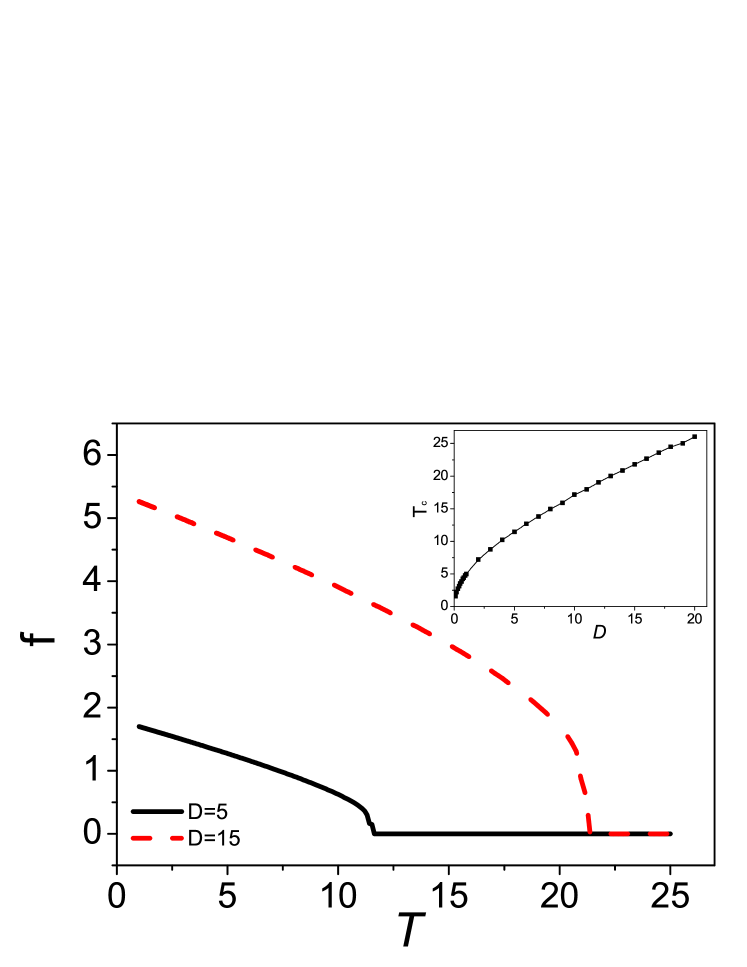
Figure 4: Effective force constant $f$ as a function of the temperature for the model (18). Inset: The critical temperature $T_{c}$, above which $f$ vanishes, against the nonlinearity $D$.

We then use Eq. (9) to compute the heat flux and compare the analytical result with numerical simulations, as shown in Fig. 5. One can see that since the nonlinearity $D$ is weak, the heat flux increases monotonically with increasing $\Delta T$ . Nevertheless, NDTR occurs as $D$ becomes large enough. Like $\phi^{4}$ model, Fig. 5 indicates that as the nonlinearity increases, the soft potential model also exhibits a transition from positive differential thermal resistance (PDTR) to NDTR.

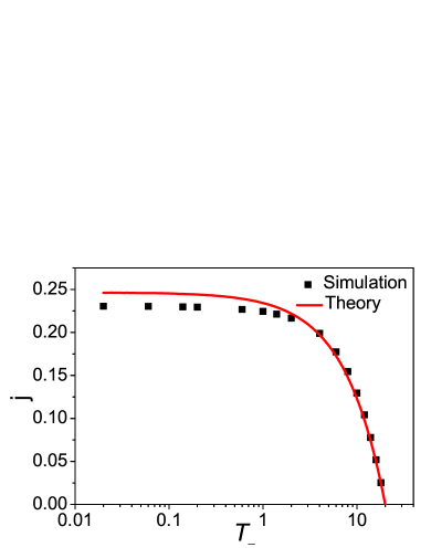
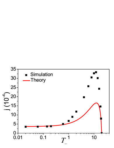
Figure 5: Heat flux $j$ as a function of $T_{-}$ for the Morse model. Left: $D=5\times 10^{-5}$; Right: $D=15$. In both cases, $\alpha=0.426$, $K_{int}=0.05$, $T_{+}=20$ and $N=64$ for the numerical simulation.

Figure 6: Morse model: The scaled turning temperature $T^{*}/T_{+}$, at which the heat current exhibits a maximum, as a function of $T_{+}$. Here $D=15$,$\alpha=0.426$.

A simple scaling relation like Eq. (17) for the nonlinearity and the temperature is inexistent for the Morse model. However, increasing the nonlinearity is qualitatively equivalent to increasing the temperature. Thus a similar transition from PDTR to NDTR as the temperature increases can be expected. In Fig. 6, we calculate the scaled turning point $\tau^{*}\equiv T^{*}/T_{+}$, at which the heat flux exhibits a maximum. Non-zero $\tau^{*}$ indicates the presence of NDTR. The analytical result shows the on-set of NDTR at $T_{+}\approx 11$ for the dissociation threshold fixed at $D=15$.

However, one should note that the SCPT fails in the vicinity of the melting transition for the present soft potential model, as pointed out in Ref. Dauxois et al. (1993). The reason for the failure of the variational approach is the fact that the half-bounded potential (18) cannot be simply approximated by the trial harmonic potential with a temperature-dependent force constant. This pecularity prevents us from modelling the crucial role of the nonlinearity in this regime using the SCPT. This point will be discussed in detail in the next section. Although it is clear that the quantitative agreement with the simulation result is poor, we emphasize that the present approach goes far beyond the traditional Landauer approach in its ability to characterize the nonlinear response regime, for which a transition from PDTR to NDTR is illustrated at least in a qualitative manner.

III Physical Mechanism

The results presented so far give rise to the following question: what is the origin of NDTR in the above models? We will show that the classical Landauer equation (9) yields a simple and intuitive explanation. One should note that the temperature discontinuity at the virtual interface(the site $x_{0}$) indicates the existence of the thermal boundary resistance (or conductance, see Ref. Swartz and Pohl (1989)), and it plays a crucial role for the heat conduction in our weakly-coupled model. Defining the effective thermal boundary conductance by

$$\sigma=\frac{k_{B}}{2\pi}\int_{\omega_{min}}^{\omega_{max}}\mathcal{T}(\omega)\,\mathrm{d}\omega,$$ (20)

Eq. (9) can be rewritten as

$$j=\Delta T\sigma,$$ (21)

which is similar in form to Ohm’s law for electrical conduction. The simple relation  (21) suggests that there exists mainly two contributions to the temperature dependence of the heat current for a two-segment system. The first contribution comes from the temperature difference $\Delta T$, which acts as an external thermal force and yields the regularly increasing behavior of $j$ with decreasing $T_{-}$. The second contribution is due to the thermal boundary conductance $\sigma$. One can see from Fig. 7 that unlike $\Delta T$, $\sigma$ is an increasing function of $T_{-}$. The widening of the overlap band of the vibrational spectrum of segments $L$ and $R$, or $\Delta\omega=\omega_{max}-\omega_{min}$, is mainly responsible for this increasing behavior of the thermal conductance. Consequently, the origin of NDTR effect is basically the competition between the growing “external field” $\Delta T$ and the diminishing overlap band $\Delta\omega$ as $T_{-}$ decreases. NDTR thus occurs below the temperature $T^{*}$ at which the opposite behavior of both contributions exactly compensate each other and it takes place if and only if $\sigma$ becomes dominant for $T_{-}<T_{+}$. Fig. 7 shows the apparition of NDTR effect as one considers different nonlinearity parameters $\lambda=1,4,9$ for the $\phi^{4}$ model. One can note that for segments with $\lambda$ large enough, $j$ vanishes as $T_{-}$ decreases due to the mismatch of the phonon bands. We also plot in Fig. 8 the thermal boundary conductance $\sigma$ and the corresponding heat flux $j$ for the Morse model, which displays a similar behavior. We can thus conclude that the proposed mechanism for the occurring of NDTR is valid for both hard and soft models. For the harmonic system, $\sigma$ is exactly temperature independent, leading to the linear behavior observed in Fig. 1.

One should note that the curve 2 of Fig. 8 exhibits a jump at $T_{-}=T_{c}$ . For $T_{-}\geq T_{c}$, the effective force constant $f$ vanishes and the phonon frequency becomes temperature independent. The system thus behaves like a harmonic chain, characterized by a temperature independent thermal boundary conductance $\sigma$ and a linear behavior of the heat flux. The occurrence of the jump and the exact linear behavior of the heat flux as $T_{-}\geq T_{c}$ are inconsistent with the numerical simulation. As discussed in the last section, this artificial result lies in the incapability of the SCPT to model the transition at the vicinity of $T_{c}$ as shown in Fig. 4. Since $T_{c}$ increases with $D$, the artificial jump disappears provided $T_{+}<T_{c}(D)$, which is illustrated in the right plot of Fig. 5.

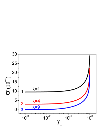
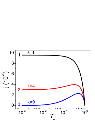
Figure 7: $\phi^{4}$ model: The thermal boundary conductance $\sigma$ (left plot) and the heat flux $j$ (right plot) against $T_{-}$ for different values of $\lambda$. Lines 1, 2, 3 correspond to $\lambda=1$, 4, 9, respectively. One can see that nonlinearity $\lambda$ has an important effect on the behavior of the heat flux due to the interchange of the dominant role in Eq. (21). Here $T_{+}=1$, $K_{int}=0.05$.

IV SUMMARY

In summary, we presented a classical Landauer formula to study NDTR effect in typical lattice models. It was shown that NDTR cannot occur in a harmonic lattice, for which the linear relation (1) is generally valid no matter how large the temperature difference is. In the presence of anharmonicity, one can observe a transition from the absence to the presence of NDTR as the nonlinearity is increased for both hard and soft potentials. The NDTR effect is basically due to the competition between the increasing behavior of the external field and the decreasing behavior of the effective thermal boundary conductance of the chain. The transition in Figs. 3 and 6 indicates that NDTR may be controlled by adjusting the parameters of the system or the temperature of heat baths, whose utility for nanoscale applications is clear.

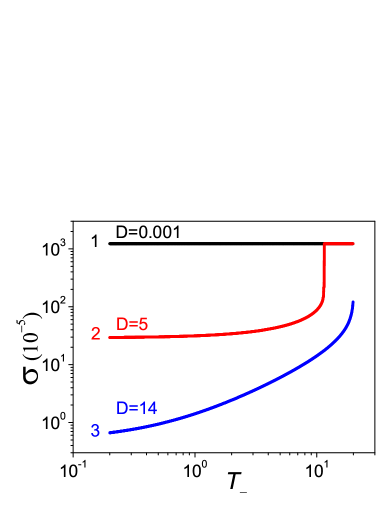
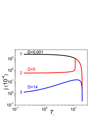
Figure 8: Morse model: The thermal boundary conductance $\sigma$ (left) and the heat flux $j$ (right) as a function of $T_{-}$ for different values of $D$. Lines 1, 2, 3 correspond to $D=0.001,5,18$, respectively. Here $T_{+}=20$, $K_{int}=0.05$.

It is imperative to clarify why we are allowed to apply such a seemingly ballistic transport formula (9) to calculate the heat flux through a nonlinear system in the strong field regime. For the particular model presented, even though the whole system is at strong external field, each segment is still close to its corresponding equilibrium state thanks to the weak coupling, and can thus be approximately described by SCPT. It should be stressed that the analytical estimation, which is based on the local thermal equilibrium of the segments, holds only if the coupling $K_{int}$ is weak enough. For strong coupling, both segments get far from thermal equilibrium and SCPT can not be applied anymore to deal with the nonlinearity.

Finally, it is worth giving a comment about the relation between asymmetric heat conduction and NDTR. Note the following two facts: 1) Asymmetric heat conduction results from the intrinsic spatial asymmetry of the model, which is not necessary for the occurring of NDTR as shown in this study; 2) One can observe asymmetric heat conduction without the occurring of NDTR as long as the applied temperature difference is moderate. It seems that the NDTR, as a field-induced effect, is neither a sufficient nor a necessary condition for thermal rectification.