Synoptic Sky Surveys and the Diffuse Supernova Neutrino Background:
Removing Astrophysical Uncertainties and Revealing Invisible Supernovae

Abstract

The cumulative (anti)neutrino production from all core-collapse supernovae within our cosmic horizon gives rise to the diffuse supernova neutrino background (DSNB), which is on the verge of detectability. The observed flux depends on supernova physics, but also on the cosmic history of supernova explosions; currently, the cosmic supernova rate introduces a substantial ($\pm 40\%$) uncertainty, largely through its absolute normalization. However, a new class of wide-field, repeated-scan (synoptic) optical sky surveys is coming online, and will map the sky in the time domain with unprecedented depth, completeness, and dynamic range. We show that these surveys will obtain the cosmic supernova rate by direct counting, in an unbiased way and with high statistics, and thus will allow for precise predictions of the DSNB. Upcoming sky surveys will substantially reduce the uncertainties in the DSNB source history to an anticipated $\pm 5\%$ that is dominated by systematics, so that the observed high-energy flux thus will test supernova neutrino physics. The portion of the universe ($z\mathrel{\mathchoice{\lower 3.6pt\vbox{\halign{$\mathsurround=0pt\displaystyle\hfil#\hfil$\cr<\crcr\sim\crcr}}}{\lower 3.6pt\vbox{\halign{$\mathsurround=0pt\textstyle\hfil#\hfil$\cr<\crcr\sim\crcr}}}{\lower 3.6pt\vbox{\halign{$\mathsurround=0pt\scriptstyle\hfil#\hfil$\cr<\crcr\sim\crcr}}}{\lower 3.6pt\vbox{\halign{$\mathsurround=0pt\scriptscriptstyle\hfil#\hfil$\cr<\crcr\sim\crcr}}}}1$) accessible to upcoming sky surveys includes the progenitors of a large fraction ($\simeq 87\%$) of the expected 10 – 26 MeV DSNB event rate. We show that precision determination of the (optically detected) cosmic supernova history will also make the DSNB into a strong probe of an extra flux of neutrinos from optically invisible supernovae, which may be unseen either due to unexpected large dust obscuration in host galaxies, or because some core-collapse events proceed directly to black hole formation and fail to give an optical outburst.

I Introduction

Core-collapse supernovae are the spectacular outcome of the violent deaths of massive stars. These events, which include Type II, Type Ib, and Type Ic supernovae, are in a real sense “neutrino bombs” in which the production and emission of neutrinos dominates the dynamics and energetics. This basic picture now rests on firm observational footing in light of the detection of neutrinos from SN 1987A hirata ; bionta . Thus all massive star deaths – certainly those that yield optical explosions, and even “invisible” events that do not – are powerful neutrino sources. Yet only the very closest events can be individually detected by neutrino observatories, leading to burst rates so small that no new events have been seen in more than two decades.

All core-collapse events within the observable universe emit neutrinos whose ensemble constitutes the diffuse supernova neutrino background (DSNB) group1 ; group2 ; group3 ; daigne05 ; Strigari04 ; yuksel05 ; lunardini06 ; horiuchi . Core-collapse supernovae produce all three active neutrino species (and their antineutrinos), all in roughly equal numbers. However, for the foreseeable future only the $\bar{\nu}_{e}$ flux can be detected above backgrounds present on Earth. Specifically, the DSNB dominates the (anti)neutrino flux at Earth in the $\sim 10-26$ MeV energy range, and has long been a tantalizing signal that has become a topic of intense interest (e.g., group1 ; group2 ; group3 ; daigne05 ; Strigari04 ; yuksel05 ; lunardini06 ; horiuchi ). Until now no DSNB signal has been detected, which set an upper bound on the DSNB flux. Super-Kamiokande (Super-K) set the upper limit to be $1.2\,\rm cm^{-2}\,s^{-1}$ above 19.3 MeV of the neutrino energy malek . However, this limit is already close to theoretical prediction and thus Super-K is expecting to detect the first DSNB signal within the next several years.

Recently, Ref. horiuchi considered a variety of complementary indicators of the cosmic supernova rate, and concluded that the DSNB is no more than a factor $\sim 2-4$ below the 2003 Super-K limit malek . Moreover these authors point out that if Super-K is enhanced with gadolinium to tag detector background events beacom03 , the resulting enhanced sensitivity at 10 – 18 MeV should lead to a firm DSNB detection.

In light of the impending DSNB detection it is imperative to quantify the uncertainties in the prediction and to reduce these as much as possible. The predicted flux depends crucially on: (a) supernova neutrino physics, via the emission per supernova; and (b) the cosmic history of core-collapse supernovae, via the cosmic supernova rate (hereafter, CSNR). Our emphasis in the present paper is on the CSNR, which has begun to be measured in a qualitatively new way by “synoptic” surveys. These new campaigns repeatedly scan the sky with a certain fields of view and high sensitivity. Pioneering synoptic surveys are already in hand and have shown the power of this technique. To date, these surveys have reported the detection of several hundreds of supernovae in total, including both Type Ia and core-collapse events essence ; sdss-sn ; snls ; hst ; TSS ; pq ; ptf ; catalina . Future surveys, such as DES, Pan-STARRS, and LSST, should find $>10^{4}\ \rm CCSNe\ yr^{-1}$, eventually with detection rates of $>10^{5}\ \rm CCSNe\ yr^{-1}$ based on their depths and large fields of view lf . Current predictions show that these data will provide an absolute measurement of the CSNR to high statistical precision out to $z\sim 1$ lf ; LSSTsb . Note that observations seem to suggest that Type IIn supernovae are intrinsically the most luminous core-collapse type richardson , and therefore would contribute to most of the detections at $z\gtrsim 0.5$; but as we discuss below, the nature of the bright end of the supernova luminosity function remains uncertain and other rare but bright supernova types TSS ; SN2008es ; GalYam ; quimby might also be important at these large redshifts.

It is important to appreciate that the most crucial input from future synoptic surveys will be the normalization of the CSNR. The shape of the CSNR follows from that of the star-formation rate due to the very short lifetimes of all massive star progenitors, and the cosmic star-formation redshift history is already relatively well-known out to $z\sim 1$. However, the CSNR normalization is only known to within $\sim 40\%$. This will be greatly improved by future synoptic surveys, which should measure the CSNR to extremely high precision at $z\sim 0.3$, and therefore dramatically reduce the uncertainties in the CSNR (and hence the DSNB) normalization.

Because our focus is on the interplay between synoptic surveys and neutrino observations, we wish to carefully distinguish different outcomes for massive stars and their resulting optical and neutrino emission. All collapse events produce neutrinos; however, simulations have shown that both the amount and energies of the supernova neutrinos varies with the mass range of the progenitor stars and how they end their lives fryer99 ; daigne05 ; sumiyoshi07 ; horiuchi ; sumiyoshi08 ; nakazato ; lunardini09 . Unfortunately, there exists great uncertainty about the fate of massive stars, and the as-yet unresolved physics of the baryonic explosion mechanism may well play an important role in determining the outcomes buras05 ; janka06 ; mezzacappa ; thompson ; sumiyoshi07 . Recent work suggests that stars below some characteristic mass (estimated at $\sim 25M_{\odot}$) do explode, producing optical supernovae and leaving behind neutron stars; on the other hand, stars above some mass scale (estimated at $\sim 40M_{\odot}$) are expected to collapse directly into massive black holes without optical signals fryer99 ; heger ; nakazato . It is possible that between these regimes, a mass range exists (e.g., $25-40M_{\odot}$) that would be a gray area where core-collapses form black holes from fallback while still being able to display some (perhaps dim) optical signals.

In the following sections, we will refer to those massive stars that first undergo regular core collapse and bounce as “core-collapse” events, whether they ultimately leave behind neutron stars or black holes formed from fallback. Those massive stars that collapse directly to black holes we will refer to as “direct-collapse” events. Events that also produce substantial electromagnetic outbursts we refer to as “visible”; those that do not are “invisible.” For simplicity, but also following current thinking, we take visible events to be core-collapse events that produce neutron stars and conventional (i.e., 1987A-like) neutrino signals. We take invisible events to be direct-collapse events, which have a higher-energy neutrino signal nakazato . “Failed” supernovae should be invisible from our viewpoint, though some may have weak electromagnetic signals that we henceforth ignore macfadyen .

The focus of this paper is to quantify how the CSNR determination by future synoptic sky surveys will improve the DSNB prediction, and to point out some of the science payoff of this improvement. After summarizing the DSNB calculations (§II), we present our forecasts for the CSNR measurements by synoptic sky surveys (§III). Using these, we show the impact on the DSNB (§IV). In particular, we discuss present constraints on invisible events, and strategies for DSNB data to probe the fraction of massive star deaths that are invisible (§V). We then switch to a extremely conservative viewpoint and discuss the robust lower limit on the DSNB (§VI). Conclusions are summarized in §VII.

II DSNB Formalism and Physics Inputs

The neutrino signal from the ensemble of cosmic collapse events is conceptually simple, and is given by the line-of-sight integral of sources out to the cosmic horizon (more precisely, to the redshift where star formation begins; in practice, the result does not change once redshifts of a few are reached). The well-known result is

$$\phi_{\nu}(\epsilon) =4\pi I_{\nu}(\epsilon)=c\frac{dn_{\nu}}{d\epsilon}$$

$$=c\int_{0}^{\infty}(1+z)\ \left|\frac{dt}{dz}\right|\ {\cal R}_{\rm tot}(z)\ N_{\nu}[(1+z)\epsilon]\ dz,$$ (1)

where $I_{\nu}(\epsilon)$ is the neutrino intensity (flux per solid angle) of cosmic supernova neutrinos with observed energy $\epsilon$. Because Earth is transparent to neutrinos, detectors see a total (angle-integrated) flux $\phi_{\nu}(\epsilon)$ from the full sky. Note that neutrinos and their energies are measured individually, so the intensity and fluxes measures particle number, not the energy carried by the particles. Two source terms, ${\cal R}_{\rm tot}$ and $N_{\nu}[(1+z)\epsilon]$, appear in Eq. II. ${\cal R}_{\rm tot}$ is the cosmic rate of collapse events, i.e., the number of collapse events per comoving volume per unit time in the rest frame. Each source, i.e., each collapse event, has a neutrino energy spectrum $N_{\nu}(\epsilon_{\rm emit})$ in its emission frame with rest-frame energy $\epsilon_{\rm emit}=(1+z)\epsilon$; the factor $(1+z)$ accounts for the redshifting of energy into the observer’s frame. Because we allow for different neutrino energy spectra for core-collapse (CC) and direct-collapse (DC) events, $N_{\nu}[(1+z)\epsilon]$ can be expressed as

$$N_{\nu}[(1+z)\epsilon]=f_{\rm CC}\,N^{\rm CC}_{\nu}[(1+z)\epsilon]+f_{\rm DC}\,N^{\rm DC}_{\nu}[(1+z)\epsilon],$$ (2)

where $f_{\rm DC}={\cal R}_{\rm tot}^{\rm DC}/{\cal R}_{\rm tot}$ and $f_{\rm CC}=1-f_{\rm DC}$ are the fractions for direct-collapse and core-collapse events, respectively; we assume these to be constants independent of time and thus redshift. Because these fractions are very uncertain, below we will consider a range of possible values. Finally, for the standard $\Lambda$CDM cosmology the time interval per unit redshift is

$$\left|\frac{dt}{dz}\right| =\frac{1}{(1+z)H(z)}$$

$$=\frac{1}{(1+z)H_{0}\sqrt{\Omega_{\rm m}(1+z)^{3}+\Omega_{\Lambda}}}.$$ (3)

Equation II shows that three inputs control the DSNB: (i) cosmology, via the cosmic line integral and parameters; (ii) supernova neutrino physics, via the source spectrum. (iii) astrophysics, via the CSNR. Of these, the cosmological inputs entering via Eq. II are very well understood and their error budget is negligible. We adopt the standard $\Lambda$CDM model, with parameters from the 5-year WMAP data: $\Omega_{\rm m}=0.274$, $\Omega_{\Lambda}=0.726$, and $H_{0}=70.5\ \rm km\ s^{-1}\ Mpc^{-1}$ wmap5 . Within this fixed cosmology, DSNB predictions require knowledge of the source spectra and CSNR. The purpose of this paper is to forecast the effects of future improvements on the source rate, but to illustrate these we must adopt source spectra.

Core-collapse neutrino spectra are in principle calculable from detailed supernova simulations, e.g., buras05 ; janka06 ; mezzacappa ; thompson ; sumiyoshi07 . In practice, it remains quite difficult to simulate supernova neutrino emission accurately within realistic explosion models (if they explode at all!) and certainly it remains computationally prohibitive to perform such ab initio simulations over wide ranges of supernova progenitors. Consequently, in DSNB predictions different groups have taken different approaches in estimating neutrino energy source spectra. Here, we adopt the treatment in the recent DSNB forecasts of Ref. horiuchi . These authors approximated the neutrino energy spectra as Fermi-Dirac distributions with zero chemical potential:

$$N_{\nu}(\epsilon)={\cal E}_{\nu}\frac{120}{7\pi^{4}}\frac{\epsilon^{2}}{T^{4}_{\nu}}(e^{\epsilon/T_{\nu}}+1)^{-1},$$ (4)

where ${\cal E}_{\nu}$ is the total energy carried in the electron antineutrino flavor and $T_{\nu}$ is the effective electron antineutrino temperature. Neutrino flavor change effects are absorbed into the choices of ${\cal E}_{\nu}$ and $T_{\nu}$. Following Ref. horiuchi , we assume the total energy is equally partitioned between each neutrino flavor for both core-collapse and direct-collapse events, i.e. ${\cal E}_{\nu}={\cal E}_{\nu,\rm tot}/6$ for individual neutrino flavor, where ${\cal E}_{\nu,\rm tot}$ is the total (all-species) energy output. The variation in neutrino emission from different core-collapse progenitor stars is in general expected to be small because neutrinos come from newly-formed neutron stars. We adopt ${\cal E}_{\nu,\rm tot}=3\times 10^{53}$ erg per core-collapse event. Ref. horiuchi finds that the average temperature after neutrino mixing is constrained to lie in the range $T_{\nu}\sim 4-8\ \rm MeV$. We choose $T_{\nu}=4\ \rm MeV$ as our benchmark temperature, which is close to the empirically-derived spectrum of SN 1987A yuksel07 .

For the direct-collapse events, hydrodynamic simulations show that the neutrino spectra are sensitive to the progenitor masses and nuclear equation of states, with models giving total neutrino energy outputs ranging from $1.31\times 10^{53}$ to $5.15\times 10^{53}$ erg and different neutrino average energies ranging from $\epsilon^{\rm avg}_{\nu}$ = 18.6 to 23.6 MeV sumiyoshi07 ; sumiyoshi08 ; nakazato . We choose the model with higher energy so it will create a greater difference for comparison. That is, we take ${\cal E}_{\nu,\rm tot}=5.2\times 10^{53}$ erg, and $T_{\bar{\nu}_{e}}=\epsilon^{\rm avg}_{\nu}/3.15=7.5$ MeV.

In what follows, we first take all supernovae to be core-collapse events (thus visible) as the fiducial case, and then we will examine the impact of the direct collapse (invisible) supernova scenario. Since the emission from the direct-collapse events is taken to be larger, this will increase the DSNB detection rates. Cosmic supernova neutrinos will be detected mainly via inverse beta decay $\bar{\nu_{e}}+p\rightarrow n+e^{+}$ interactions with protons in a liquid water or scintillator detector. This reaction is endoergic with the threshold energy of 1.8 MeV. To a good approximation, the nucleon remains at rest, so that $\epsilon_{e^{+}}\simeq\epsilon-\Delta$, where $\epsilon_{e^{+}}$ is the positron total energy, $\epsilon$ is the $\bar{\nu}_{e}$ energy, and $\Delta=m_{n}-m_{p}=1.295$ MeV. The expected differential event rate, per unit time and energy, is

$$\frac{dR_{\rm detect}}{d\epsilon}=N_{p}\ \sigma_{\nu p}(\epsilon)\ \phi_{\nu}(\epsilon)\ \ .$$ (5)

The well-known inverse beta decay cross section $\sigma_{\nu p}(\epsilon)$ vogel ; strumia , taken here at lowest order, and which increases with energy roughly as $\epsilon^{2}$. Thus the event rates give larger weight to the high-energy neutrino flux, which, as we will see is the regime best probed by supernova surveys. The total event rate in a detector sensitive to neutrino energies $\epsilon$ is thus $R=\int^{\epsilon_{\rm max}}_{\epsilon_{\rm min}}dR/d\epsilon\;d\epsilon$. The factor $N_{p}$ in Eq. 5 gives the number of free protons (those in hydrogen atoms) in the detector; in our calculations, we use the value corresponding to 22.5 kton of pure water for Super-K.

The upper panel of Fig. 1 shows the neutrino event rate – the integrand of Eq. (1) with $T_{\nu}$ = 4 MeV – with respect to redshift at certain fixed observed energies. Because of redshift, neutrinos with low observed energies are more likely to come from high redshift supernovae, while neutrinos with high observed energies are more likely to come from low redshift supernovae.

A measurement of DSNB neutrinos and their energy spectrum will thus provide unique new insights into the physics of massive-star death. But for the DSNB to usefully probe the neutrino emission from supernova interiors, the cosmic source rates must be known. It is to this that we now turn.

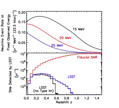
Figure 1: DSNB and synoptic survey redshift distributions. Upper Panel: The integrand of Eq. II as a function of redshift for different choices of observed neutrino energies; this shows the redshift distribution of sources that contribute to the DSNB signal at these energies. Here we assume all the supernovae are core-collapse events, as defined in §I. Bottom Panel: The blue curve is the supernova detection rate by LSST in $r$-band as a function of redshift, with survey depth $m_{\rm lim}^{\rm sn}=23^{\rm mag}$ and sky coverage of 6.1 sr (20,000 $\rm deg^{2}$). The black curve is a more conservative estimation of the LSST supernova detection rate by excluding Type IIn supernovae, which seem to be the most luminous based on the small sample of current data. The red curve is the fiducial supernova rate for comparison, which is the full-sky supernova rate without considering dust extinction or survey depth. The curves have bin size $\Delta z$ = 0.05, and the band thickness (which are in most cases thinner than the curve width) represent the statistical uncertainty $1/\sqrt{N}$.

III DSNB Astrophysics Input

The CSNR not only controls the DSNB flux, but also is of great intrinsic interest, and has a direct impact on numerous problems in cosmology and particle astrophysics. The stellar progenitors of both core-collapse and direct-collapse events are very short-lived; consequently the CSNR is closely related to the cosmic star-formation rate, which has been intensively studied for the past decade csfr . From the present epoch back to $z\sim 1$, the cosmic star-formation rate increases by an order of magnitude. At higher redshifts, $z\mathrel{\mathchoice{\lower 3.6pt\vbox{\halign{$\mathsurround=0pt\displaystyle\hfil#\hfil$\cr>\crcr\sim\crcr}}}{\lower 3.6pt\vbox{\halign{$\mathsurround=0pt\textstyle\hfil#\hfil$\cr>\crcr\sim\crcr}}}{\lower 3.6pt\vbox{\halign{$\mathsurround=0pt\scriptstyle\hfil#\hfil$\cr>\crcr\sim\crcr}}}{\lower 3.6pt\vbox{\halign{$\mathsurround=0pt\scriptscriptstyle\hfil#\hfil$\cr>\crcr\sim\crcr}}}}1$, the cosmic star-formation rate becomes less certain, but the $z\mathrel{\mathchoice{\lower 3.6pt\vbox{\halign{$\mathsurround=0pt\displaystyle\hfil#\hfil$\cr<\crcr\sim\crcr}}}{\lower 3.6pt\vbox{\halign{$\mathsurround=0pt\textstyle\hfil#\hfil$\cr<\crcr\sim\crcr}}}{\lower 3.6pt\vbox{\halign{$\mathsurround=0pt\scriptstyle\hfil#\hfil$\cr<\crcr\sim\crcr}}}{\lower 3.6pt\vbox{\halign{$\mathsurround=0pt\scriptscriptstyle\hfil#\hfil$\cr<\crcr\sim\crcr}}}}1$ regime is responsible for a large fraction of the observable DSNB signal. On the other hand, while the shape of the cosmic star-formation rate is relatively secure, the absolute normalization remains harder to pin down. Recent estimates using multiwavelength proxies for the star-formation rate indicate a $\pm 20\%$ uncertainty at $z=0$ and a larger uncertainty at higher redshift, producing an average of $\pm 40\%$ uncertainty on the DSNB detection rate horiuchi . For the direct supernova rate data reported in Ref. horiuchi , here we adopt a $\pm 40\%$ uncertainty at $z=0$, double that on the star-formation rate itself (this should not be confused with the 40% above).

Fortunately, a new generation of powerful sky surveys are poised to offer a new, high-statistics measure of the CSNR. These surveys have wide fields of view and large collecting areas, in order to produce deep scans of large portions of the sky. These synoptic surveys are designed to repeatedly scan a large portion of the sky every few nights with limiting single-exposure magnitudes of $\sim 21^{\rm mag}$ to $\sim 24^{\rm mag}$, and possibly deeper in several passbands. Relatively more modest prototype synoptic surveys have already been completed, e.g., SDSS-II sdss-sn and SNLS snls , or are underway, e.g., the Pan-STARRS 1 prototype telescope has already seen first light Tonry (2003), and the Palomar Transient Factory already reported their first results ptf . Large-scale planned surveys include DES The Dark Energy Survey Collaboration (2005), LSST The LSST Collaboration (2007); Tyson (2002), SkyMapper keller , and the full-scale Pan-STARRS.

These synoptic surveys will repeatedly scan the sky with revisit times (“cadences”) of $\sim$ few days. The cadence timescale is ideally suited for following supernova light curves and detecting events near maximum brightness. Indeed, the SNLS have reported 289 confirmed Type Ia events and 117 confirmed core-collapse supernovae out to $z\sim 0.4$ snls . SDSS-II also reported 403 spectroscopically confirmed events sdss-sn (most of which were Type Ia), and 15 confirmed Type IIp events that are potentially capable of being used as standardized candles DAndrea09 . The Palomar Transient Factory has already found quimby three events which are among the most luminous core-collapse events ever found, and which appear to be pulsational pair-instability explosions of ultramassive stars. Finally, Pan-STARRS 1 has reported its first confirmed supernova Tonry (2003).

Note that these surveys are unbiased in that they cover a large portion of the sky regions systematically and thus do not pre-select galaxy types or redshifts or luminosities for supernova monitoring, whereas most of the past supernova surveys monitored pre-selected galaxies so that the results were biased, though attempts have been made to correct for that.

Currently, most of the design efforts for synoptic surveys focus on Type Ia supernovae, because these events are a crucial cosmological distance indicator at large redshifts. However, the survey requirements for Type Ia supernova detection are also well-matched to collapse events, and therefore surveys that are tuned for Type Ia supernovae will automatically observe collapse events also. With their proposed properties, these surveys are expected to discover $\sim 10^{5}$ collapse events per year out to redshift $z\sim 1$ young08 ; lf . Due to the large sample size, spectroscopic followup is unfeasible for most events, so photometric redshifts of the host galaxies (for which deep co-added fluxes will be available) or of the supernovae themselves will be needed, just as in the case of Type Ia events zheng .

Lien & Fields lf give detailed predictions for the supernova harvest by synoptic surveys; here we summarize the key factors important for the DSNB. Within the 5-color SDSS $ugriz$ bandpass system, the $r$ and $g$ bands provide the largest supernova harvest, due largely to high detector efficiency for these wavelengths. Moreover, distant intrinsically blue collapse events are redshifted into these bands. Detection of a supernova is done by differencing exposures of the same field of view. To determine if a transient is a supernova and to establish its type, one must follow the supernova through the rise and fall of its light curve. Consequently the peak flux must be brighter than the minimum flux for point source detections, and following Ref. lf we set a supernova limiting magnitude $m_{\rm lim}^{\rm sn}=m_{\rm lim}-1^{\rm mag}$ that is brighter by $1^{\rm mag}$ than the single-visit point-source limit $m_{\rm lim}$. Finally, for a given scan cadence timescale, a survey must trade off scan area $\Delta\Omega_{\rm scan}$ and exposure depth $m_{\rm lim}^{\rm sn}$. Surveys with large scan area, such as Pan-STARRS and LSST, are planned to have survey depth $m_{\rm lim}^{\rm sn}=23^{\rm mag}$.

The blue curve in the lower panel of Fig. 1 plots the expected collapse event rate detected by LSST in $r$-band. One can see from the plot that in one year, LSST will have more than 100 supernova detections in all $\Delta z=0.05$ redshift bins out to redshift $z\sim 0.9$, and for $z\simeq 0.1-0.5$, LSST will be able to detect more than $10^{4}$ supernovae in each bin. Ref. lf shows that Type IIn supernovae contribute to most of the detections for $z\gtrsim 0.5$ based on the luminosity functions provided in Ref. richardson . Since this higher end of the detection redshift range is highly affected by the small sample of Type IIn in Ref. richardson , we also plot the black curve for reference to show a more conservative estimation that excludes Type IIn supernovae. One can see that the detection would reach $z\sim 0.6$ in this case. The thickness of the blue and black curve represent the statistical uncertainty ($1/\sqrt{N}$), which in most cases are thinner than the curve width because the uncertainty is very small due to the large number of supernovae. The full-sky fiducial supernova rate based on Ref. horiuchi is also plotted for comparison. The difference between the fiducial supernova rate and the LSST detection rate is mainly due to survey depth (magnitude/flux limit), sky coverage and to a lesser extent dust obscuration.

A high precision measurement of the CSNR can therefore be done via direct counting of the enormous number of collapse events versus redshift. While a measurement of the CSNR shape will tests the consistency with results inferred from other methods, such as the star-formation history, the real power of synoptic surveys will be the high-statistics determination of the CSNR normalization. Note that this can in principle be determined by precision measurement of the CSNR at a single redshift bin, where the counts are largest. For a large survey like LSST, this should occur around $z\sim 0.3$, which is set by the tradeoff of survey volume and limiting magnitudes lf . In general, LSST is expected to probe the CSNR out to redshift $z\sim 0.9$ to $1/\sqrt{N}\sim 10\%$ statistical precision within one year of observation.

As mentioned earlier, detections in the $z\sim 0.5-0.9$ range will be dominated by the most luminous core-collapse events. In a study of the core-collapse luminosity function based on relatively sparse and inhomogeneously taken data, the relatively rare Type IIn events were found to be the most intrinsically luminous richardson ; and ultraluminous Type IIn events have been found SNIIn . Recent observations, including those by the synoptic Palomar Transient Factory and by ROTSE-III/Texas Supernova Search, show that other core-collapse types can also lead to ultraluminous explosions; of these, the newly-discovered pair-instability outbursts are particularly intriguing and encouraging because this entire class of events has likely gone unnoticed until now TSS ; SN2008es ; GalYam ; quimby . There is clearly much more to be learned about about the bright end of the supernova luminosity function. As more data of these ultraluminous events become available, the redshift reach of synoptic surveys will come into a much better focus.

IV Impact of Synoptic Surveys on the DSNB

We are now in a position to assess the synoptic survey impact on the DSNB. Our viewpoint is to envision the situation several years from now, when synoptic surveys have been running in earnest, and when the DSNB signal has been at last detected. Of course, real surveys will miss core-collapse events for a variety of reasons, yet following Ref. lf we believe there is good reason to expect that these losses can be calibrated, empirically or semi-empirically, and thus the absolute CSNR can be obtained out to $z\mathrel{\mathchoice{\lower 3.6pt\vbox{\halign{$\mathsurround=0pt\displaystyle\hfil#\hfil$\cr<\crcr\sim\crcr}}}{\lower 3.6pt\vbox{\halign{$\mathsurround=0pt\textstyle\hfil#\hfil$\cr<\crcr\sim\crcr}}}{\lower 3.6pt\vbox{\halign{$\mathsurround=0pt\scriptstyle\hfil#\hfil$\cr<\crcr\sim\crcr}}}{\lower 3.6pt\vbox{\halign{$\mathsurround=0pt\scriptscriptstyle\hfil#\hfil$\cr<\crcr\sim\crcr}}}}1$; this should verify the already well-determined shape of the cosmic star-formation rate in this regime. Furthermore, surveys will definitely measure the low-redshift normalization of the CSNR to high precision via direct counting.

To be sure, it will be far from trivial to arrive at the understanding we presuppose. There will be formidable astrophysical challenges in extracting from survey data the supernova properties of interest, most importantly the event type, redshifts, and obscuration; less crucially for our purposes one would like as well the intrinsic luminosity. Ref. lf discusses some reasons for optimism in the face of these challenges, and we also remind the reader that these issues are crucial not only for studies of the DSNB but also are central for other key topics in astrophysics and cosmology. Most notably, the problems of obtaining supernova type, redshift, and obscuration are at least as pressing (and in some respects more challenging) when one uses supernovae as cosmological distance indicators and thus as probes of dark energy. Put differently, if survey supernovae are understood well enough to do dark energy cosmology, then we expect that the star-formation rate should be well-understood enough to give the DSNB source history out to $z\sim 1$, and the CSNR normalization to high precision.

We now explore the impact of a CSNR determination of this kind. That is, we assume that one can use synoptic surveys to infer the absolute normalization and shape of the CSNR out to some redshift $z_{\rm max}$. In particular, Ref. lf showed that all core-collapse types should be visible out to $z_{\rm max}\mathrel{\mathchoice{\lower 3.6pt\vbox{\halign{$\mathsurround=0pt\displaystyle\hfil#\hfil$\cr>\crcr\sim\crcr}}}{\lower 3.6pt\vbox{\halign{$\mathsurround=0pt\textstyle\hfil#\hfil$\cr>\crcr\sim\crcr}}}{\lower 3.6pt\vbox{\halign{$\mathsurround=0pt\scriptstyle\hfil#\hfil$\cr>\crcr\sim\crcr}}}{\lower 3.6pt\vbox{\halign{$\mathsurround=0pt\scriptscriptstyle\hfil#\hfil$\cr>\crcr\sim\crcr}}}}0.5$, and the very bright Type IIn events should extend to $z_{\rm max}\mathrel{\mathchoice{\lower 3.6pt\vbox{\halign{$\mathsurround=0pt\displaystyle\hfil#\hfil$\cr>\crcr\sim\crcr}}}{\lower 3.6pt\vbox{\halign{$\mathsurround=0pt\textstyle\hfil#\hfil$\cr>\crcr\sim\crcr}}}{\lower 3.6pt\vbox{\halign{$\mathsurround=0pt\scriptstyle\hfil#\hfil$\cr>\crcr\sim\crcr}}}{\lower 3.6pt\vbox{\halign{$\mathsurround=0pt\scriptscriptstyle\hfil#\hfil$\cr>\crcr\sim\crcr}}}}1$ SNIIn ; cooke . Thus we will take the CSNR shape to be directly known from surveys to $z=1$, and following Ref. lf we assume that the normalization will be very well-determined statistically, and so we will anticipate a measurement good to $\delta{\cal R}_{\rm tot}/{\cal R}_{\rm tot}=5\%$; this error would be dominated by systematic uncertainties at the most relevant redshifts.

Referring again to Fig. 1, we compare the redshift reach of synoptic surveys with the redshift distribution of the DSNB sources. We see that the two are well matched. That is, within the detection energy range ($\sim 10-26$ MeV positron energy), the neutrino sources peak within the redshift range of upcoming supernova surveys. Quantitatively, the detection rate is about 1.8 neutrinos/year within the detector energy range of 10 – 26 MeV positron energy for neutrinos from all redshifts (i.e., $z_{\rm max}=6$). Of this total rate, events within redshift $z=1$ contribute 1.5 (87%) neutrinos/year, and events within redshift $z=0.5$ contribute 1.0 (54%) neutrinos/year. Our results are in good agreement with the numbers shown in Ref. horiuchi and ando . Therefore a large fraction of the observable neutrinos come from events within $z\sim 1$, which is about the same redshift range as the upcoming supernova surveys.

We thus see that using supernovae to directly infer the CSNR allows us to robustly predict a large fraction of the detectable neutrino events. A high precision measurement of the CSNR would therefore put a better constraint on the DSNB flux, which encodes knowledge of supernova neutrino physics. For example, one would then be able to distinguish the difference between neutrino models with different effective temperatures, as demonstrated in Fig. 2.

Figure 2 plots the neutrino detection rates estimated based on models with different neutrino effective temperatures ($T_{\nu}$ = 4, 6, 8 MeV, respectively) versus neutrino energy in the observer’s frame. The upper panel shows the current $\delta{\cal R}_{\rm tot}/{\cal R}_{\rm tot}$ = 40% uncertainty in the cosmic supernova rate normalization. The bottom panel shows the future normalization uncertainty of $\delta{\cal R}_{\rm tot}/{\cal R}_{\rm tot}$ = 5% (dominated by systematics), which would be achieved within one year observation of the upcoming supernova surveys. One can see that it is not easy to distinguish different neutrino models with the current 40% uncertainty. However, with a future 5% precision, it would be certainly possible to distinguish the differences between each models and therefore provide a way to study supernova neutrino physics by combining neutrino detections and supernova surveys.

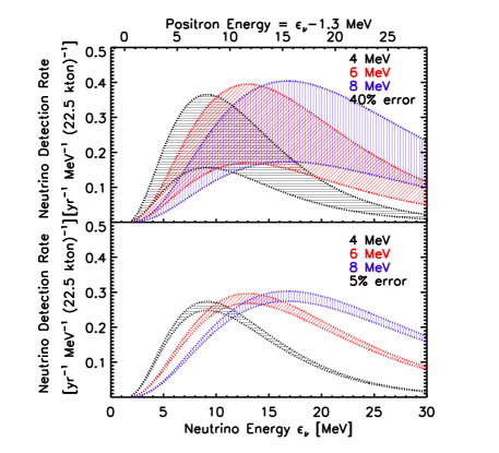
Figure 2: Upper Panel: Neutrino detection rate as a function of neutrino observed energy, with different neutrino effective temperatures are plotted for comparison. The band thickness of the curves represent a $\delta{\cal R}_{\rm tot}/{\cal R}_{\rm tot}$ = 40% uncertainty in the current CSNR normalization. Bottom Panel: Same as the upper panel, but with a 5% normalization uncertainty instead, which is the uncertainty expected from upcoming supernova surveys with one year observations.

Moreover, after several years of exposure, one might hope to attain statistics sufficient to measure the difference between the observed flux and the contributions from lower-redshift epochs sampled by survey supernovae. This difference encodes a wealth of interesting physics and astrophysics.

V Invisible Supernovae Revealed

The most dramatic possibility for a mismatch between the neutrino and optical supernova measures would reflect a real lack of optical explosions due to “invisible” supernovae. As mentioned in Section II, even in the context of conventional models there is a great uncertainty about whether stars with masses between 25 to 40 $M_{\odot}$ explode or not. A Salpeter initial mass function $dN_{\star}/dm\propto m^{-2.35}$ salpeter , dictates that for collapse events in the $8-100M_{\odot}$ range, $\sim$ 90% are core-collapse events (masses $\mathrel{\mathchoice{\lower 3.6pt\vbox{\halign{$\mathsurround=0pt\displaystyle\hfil#\hfil$\cr<\crcr\sim\crcr}}}{\lower 3.6pt\vbox{\halign{$\mathsurround=0pt\textstyle\hfil#\hfil$\cr<\crcr\sim\crcr}}}{\lower 3.6pt\vbox{\halign{$\mathsurround=0pt\scriptstyle\hfil#\hfil$\cr<\crcr\sim\crcr}}}{\lower 3.6pt\vbox{\halign{$\mathsurround=0pt\scriptscriptstyle\hfil#\hfil$\cr<\crcr\sim\crcr}}}}40M_{\odot}$), which in our assumption make optically luminous explosions even for those that form black holes from fallback, and $\sim$ 10% are direct-collapse events ($\mathrel{\mathchoice{\lower 3.6pt\vbox{\halign{$\mathsurround=0pt\displaystyle\hfil#\hfil$\cr>\crcr\sim\crcr}}}{\lower 3.6pt\vbox{\halign{$\mathsurround=0pt\textstyle\hfil#\hfil$\cr>\crcr\sim\crcr}}}{\lower 3.6pt\vbox{\halign{$\mathsurround=0pt\scriptstyle\hfil#\hfil$\cr>\crcr\sim\crcr}}}{\lower 3.6pt\vbox{\halign{$\mathsurround=0pt\scriptscriptstyle\hfil#\hfil$\cr>\crcr\sim\crcr}}}}40M_{\odot}$) that are optically invisible, but have larger neutrino emission with greater total energy ${\cal E}_{\nu,\rm tot}$ and higher neutrino average temperature $T_{\nu}$. A relatively conservative case, which has recently been studied by Lunardini lunardini09 , would then assume that around 10% of collapse events failed to explode, hence one would expect that the neutrino flux from neutrino detectors would at least be $\sim 10\%$ higher than neutrino flux from supernova surveys.

However, there remain large uncertainties in our qualitative understanding of massive star death, not to mention even larger quantitative uncertainties in neutrino and photon outputs. If, as expected, the neutrino emission is larger for these events than for ordinary supernovae, then the signal increase in the detectors can be significantly larger daigne05 ; lunardini06 ; sumiyoshi07 ; horiuchi ; sumiyoshi08 ; nakazato ; lunardini09 . Given these substantial uncertainties it is entirely possible that the invisible fraction is much higher than 10%. For example, one possible scenario is that supernovae that form black holes from fallback might actually belong to the invisible events category. Ref. fryer09 predicts the light curves of these fallback events with peak magnitudes around $V=-13$ to $-15$, which correspond to luminosities several orders of magnitude lower than ordinary core-collapse events. These authors also suggest that the total neutrino emission from the fallback events can be larger than normal supernovae fryer07 . Thus if we treat the fallback supernovae as invisible events with larger neutrino emission, the invisible fraction will be higher than current estimates would suggests lunardini09 . Therefore we will take the invisible fraction as an a priori free parameter, and explore constraints based on neutrinos and other observables.

Fig. 3 shows several constraints on the visible supernova rate ${\cal R}_{\rm vis}$ and invisible supernova rate ${\cal R}_{\rm invis}$ at $z=0$. These constraints are estimated based on current data with the assumption that the shape of the CSNR is known, and we adopt the fiducial model described in Ref. horiuchi . Blue regions in the plot represent the allowed regions; the gray region represents the explicit exclusion from the non-observation of neutrinos; and white regions represent areas that are disallowed implicitly, that is, they lie outside of current allow regions but are not banned directly based on current limits.

One way to constrain ${\cal R}_{\rm tot}$ is using the current observed cosmic star-formation rate. The ratio of massive star counts per unit mass into all stars depends only on the choice of initial mass function; we take this ratio to be $0.007/M_{\odot}$ assuming the Salpeter Initial Mass Function (IMF) salpeter . With the uncertainty $\sim 20\%$ in the cosmic star-formation rate normalization horiuchi , the upper and lower limit of current star formation rate at $z=0$ correspond to ${\cal R}_{\rm tot}(0)=1.25\pm 0.25\times 10^{-4}\,\rm yr^{-1}\,Mpc^{-3}$. respectively, which set the darker blue region in Fig. 3. Also, the present observed CSNR with $\sim 40\%$ uncertainty in its normalization is plotted as the light-blue region in Fig. 3, which correspond to the value of ${\cal R}_{\rm tot}(0)=1.25\pm 0.50\times 10^{-4}\,\rm yr^{-1}\,Mpc^{-3}$.

The DSNB limit in Fig. 3 shows the constraint estimated from the current non-detection of the supernova neutrino background, which sets an upper bound of the total core-collapse supernova rate ${\cal R}_{\rm tot}={\cal R}_{\rm vis}+{\cal R}_{\rm invis}$. Ref. yuksel05 points out that the upper limit on the neutrino flux set by Super-K in 2003 corresponds to an upper limit of 2 events per year for a 22.5 kton detector in the energy range of 18 – 26 MeV (see also Ref. lunardini_peres for the temperature dependence of the Super-K limits in terms of flux instead of event rate). For the benchmark $T_{\nu}$ = 4 MeV case, this limit allows the current ${\cal R}_{\rm tot}$ to be 4.7 times bigger than current fiducial value if we assume all neutrino emission comes from visible events. On the other hand, the Super-K limit implies a current ${\cal R}_{\rm tot}$ that is 0.64 times smaller than our fiducial value if all neutrino emission comes from invisible events. Note that these two factors are not the same because there is more neutrino emission per invisible event.

The DSNB constraint has substantial uncertainties from both the visible and invisible supernova contributions. The neutrino emission from visible events depends on the neutrino emission spectrum, i.e., temperature. To illustrate how this would change the DSNB limit, we also plotted the DSNB limit when assuming visible events have $T_{\nu}$ = 6 MeV instead of 4 MeV. The 6 MeV line intersects the ${\cal R}_{\rm vis}$ axis at 1.9 instead of 5.8 for the 4 MeV line. While the uncertainty in the neutrino emission from visible events would affect where the DSNB limit intersect with the ${\cal R}_{\rm vis}$ axis, the uncertainty in the neutrino emission from invisible events would change where the limit intersects with the ${\cal R}_{\rm invis}$ axis. In this paper we adopt the highest-energy case for the neutrino emission from invisible events; however, if we choose the lowest-energy case in Ref. nakazato , then the limit would intersect with the ${\cal R}_{\rm invis}$ axis at 4.6 and the whole region shown in Fig. 3 would be allowed by this limit and thus would give a weaker constraint.

In addition to constraints based on current observational data, Kochanek et al. proposed new method of probing invisible supernovae kochanek . These authors suggested monitoring a million supergiants, in galaxies within 10 Mpc. Because the supergiant phase lasts $\sim 10^{6}$ years, every year about one monitored supergiant will end its life. While some events will result in an ordinary optically bright supernovae, if any events lack optical outbursts – and are thus invisible by our definition – they will simply disappear in sight. Considering that the local cosmic star-formation rate is about two times higher than the cosmic average, the lowest invisible event rate that predicts one disappearing event in the proposed five years observation is around ${\cal R}_{\rm invis}=0.25\times 10^{-4}\,\rm yr^{-1}\,Mpc^{-3}$. This line is shown as the horizontal line labeled as sensitivity to stellar disappearance in Fig. 3.

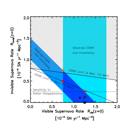
Figure 3: Summary of current and future constraints on the invisible supernova rate ${\cal R}_{\rm invis}$ (i.e. the direct-collapse event rate in our assumption) and the visible supernova rate ${\cal R}_{\rm vis}$ (i.e. the core-collapse event rate in our assumption). Blue regions are those allowed by current observed cosmic star-formation rate (CSFR) and CSNR and their uncertainties. The grey-lined region is disallowed based on the non-detection of the DSNB by Super-K with the assumption that $T_{\nu}$ = 4 MeV for visible events and 7.5 MeV (and also a higher total energy) for invisible events. Another DSNB limit with $T_{\nu}$ = 6 MeV instead of 4 MeV is also plotted for comparison. The horizontal dashed line shows the sensitivity to stellar disappearance, which will directly probe the invisible supernova rate kochanek . Note circles explored in Fig. 4 and stars in Fig. 5. Square marks a baseline shown in Fig. 4 and 5.

Despite the preliminary nature of some of the constraints in Fig  3, several interesting trends already emerge. The allowed region for invisible supernovae is nonzero, but it is bounded and cannot be arbitrarily large. Future observations will severely restrict the allowed region for visible supernovae. Obviously, the mere demonstration that ${\cal R}_{\rm invis}$ is nonzero would immediately offer novel and unique insight into supernova physics. Moreover, any quantitative determination of the absolute value of ${\cal R}_{\rm invis}$ or the ratio ${\cal R}_{\rm invis}/{\cal R}_{\rm vis}$ would give detailed insight into the explosion mechanism over the full range of core-collapse events.

Also, Fig. 3 allows a larger invisible fraction than the $f_{\rm invis}=10\%$ predicted from current theory. We marked several possible invisible fractions that we will discuss more in the figures below. The square represents a baseline, with invisible fraction $f_{\rm invis}=0\%$. Circles mark possible $f_{\rm invis}$ assuming the total CSNR is fixed to the fiducial number of ${\cal R}_{\rm tot}=1.25\times 10^{-4}\,\rm yr^{-1}\,Mpc^{-3}$. The purple circle is the conservative case with $f_{\rm invis}=10\%$, and red circle marked the highest invisible fraction ($f_{\rm invis}=40\%$) one can reach with ${\cal R}_{\rm tot}$ fixed. The corresponding changes in the DSNB detection are shown in Figure 4, where we see that when error in ${\cal R}_{\rm vis}$ drops to 5%, it will become possible to tell the difference between these three cases in the detectable neutrino energy range. The energy dependence of the fraction traces back to the higher energy of the neutrino flux from black hole forming supernovae. Therefore invisible events contribute a larger fraction of the neutrino flux at higher neutrino energy.

Another set of key points in Fig. 3 are marked with stars. In choosing these points, we allow for the uncertainties in ${\cal R}_{\rm vis}$ in order to explore even higher possible $f_{\rm invis}$ values while staying within current limits. If the visible event rate is fixed to the fiducial number of ${\cal R}_{\rm vis}=1.25\times 10^{-4}\,\rm yr^{-1}\,Mpc^{-3}$, then the purple star marks the point with $f_{\rm invis}=10\%$ adding to current fiducial ${\cal R}_{\rm vis}$, and the red star marks the point with $f_{\rm invis}=17\%$, which is the highest $f_{\rm invis}$ one can reach with ${\cal R}_{\rm vis}$ fixed. However, the visible event rate is quite uncertain and could fall substantially below our fiducial value. Including this uncertainty, the highest $f_{\rm invis}$ that is allowed by current limit is around the point marked by the orange star with $f_{\rm invis}=50\%$. Note that this point seems to lie just outside the DSNB constraint, however, one should keep in mind that the DSNB constraint is very sensible to theoretical assumption of the supernova neutrino emission and hence has its own uncertainty, as discussed earlier.

The DSNB detections corresponding to the points marked by stars are shown in Figure 5. Note that the black curve with $f_{\rm invis}=0\%$ represents the neutrino detections from the visible events, and thus is the one that would be estimated by supernova surveys; the purple and red curves include different fractions of invisible events on top of the visible events, which represent those that would be detected by neutrino detectors. Therefore Fig. 5 illustrates how the differences between DSNB from neutrino detectors and supernova surveys would encode information of the fraction of invisible events. Again, the band thickness in this figure indicates the expected 5% uncertainty in ${\cal R}_{\rm vis}$, and it is clear that these three cases will be distinguishable. The DSNB detections for the very extreme case with $f_{\rm invis}=50\%$ is plotted as the orange curve for comparison.

A 50% invisible event fraction would lead to a significant difference between flux from neutrino detectors and supernova surveys. We find that neutrinos due to invisible events within $z\sim 1$ would contribute around 75% of the event rate in the detectable energy range. For comparison, we expect the neutrinos associated with dust-obscured supernovae to be about $\sim 20\%$ of the signal. Thus, if the invisible event fraction approaches current limits, the neutrino census of supernovae should be able to rapidly and strongly point to the large contribution from these events. Additionally, an invisible event fraction of 50% could push the mass limit of the direct-collapse events to as low as $\sim$ 14 $M_{\odot}$ with the Salpeter IMF. However, theories about supernova progenitors remain quite uncertain and therefore the lower mass limit implied by the invisible fraction is also not necessarily well-defined. Once the upcoming surveys put better constraints on the invisible fraction, one can hope to learn more about the mass limit of direct-collapse events.

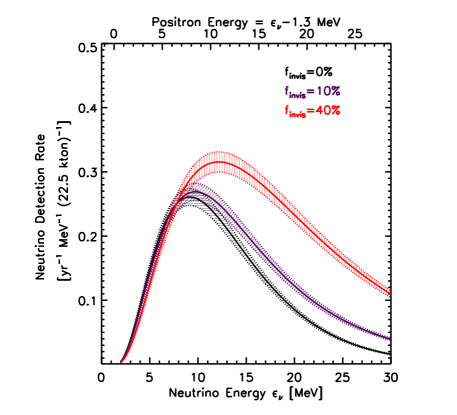
Figure 4: One year neutrino detection as a function of neutrino observed energy. Three different fractions of the invisible events are plotted with ${\cal R}_{\rm tot}$ fixed to the fiducial number. Curves with different colors correspond to the square/circles with the same color in Fig. 3. The band thickness of the curves represent 5% uncertainty expected from upcoming supernova surveys.

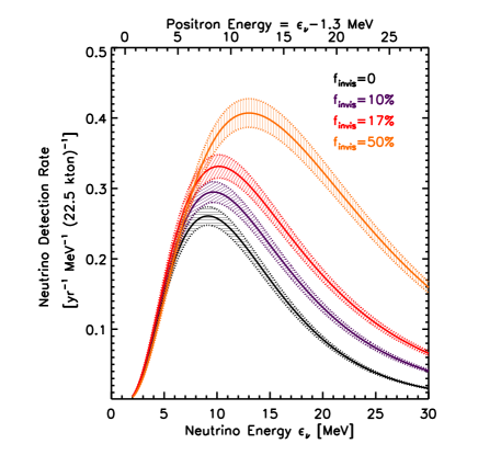
Figure 5: Similar to Fig. 4. However, we allow larger numbers for ${\cal R}_{\rm tot}$. Curves with different colors correspond to square/stars in Fig. 3. The band thickness of the curves represent 5% uncertainty expected from upcoming supernova surveys.

VI Astrophysical Challenges and Payoffs

Our discussion until now has taken a point of view that by the time synoptic surveys are well under way, the loss of supernova detections from dust and survey depth can be corrected, either using the survey data themselves or from followup observations. In this section, we change our viewpoint from this optimistic, wide-ranging anticipation of future progress to a more restricted focus on the power of the survey-detected supernovae alone.

For real surveys, some of the collapse events must be lost from detection mainly due to three factors: survey limiting magnitude, dust obscuration, and the invisible events without optical explosions. On the other hand, neutrino detection will be unaffected by any of these issues. Therefore, neutrino flux from neutrino detectors should exceed that estimated from supernova surveys.

Supernova surveys thus provide a totally empirical, model-independent method to estimate the extreme lower limit to the DSNB by simply adding up the neutrino contribution from each supernova detected. The resulting lower bound to the DSNB flux is

$$\phi_{\nu}^{\rm min}(\epsilon)\equiv\phi_{\nu}^{\rm survey}(\epsilon)=\frac{4\pi}{\Delta\Omega_{\rm scan}\Delta t}\ \sum^{\rm survey\ SNe}_{i=1}\frac{N_{\nu}[(1+z_{i})\epsilon]}{4\pi D_{L}(z_{i})^{2}}$$ (6)

where each term in the sum is the flux contributed by each supernova observed in the survey, and the prefactor includes a correction for the fraction $\Delta\Omega_{\rm scan}/4\pi$ of the sky covered by the survey. The fluxes depend on the luminosity distance $D_{L}(z)$, which is fixed by precisely known cosmological parameters. Notice that in this equation, only the neutrino energy spectrum $N_{\nu}[(1+z_{i})\epsilon$] depends on supernova and neutrino physics.

This “what you see is what you get” approach is robust but conservative. Namely, the result $\phi_{\nu}^{\rm survey}(\epsilon)$ will be an extreme lower bound for the DSNB flux. More detailed and quantitative discussion can be found in Appendix A.

Once the DSNB is detected, the difference between the detected flux and the survey-based lower bound provides a unique measure of the events unseen by surveys. For example, it is conceivable that the survey predictions could exceed the DSNB detection (or upper limit!). This result would be very surprising and thus extremely tantalizing, as it would challenge our assumptions related to supernova physics and neutrino physics. In other words, this would mean that one or both terms in Eq. 6, the luminosity distance $D_{L}$ and/or the supernova neutrino emission spectrum $N_{\nu}[(1+z_{i})\epsilon]$, might be wrong. But the physics behind $D_{L}$ rests on well-established Friedmann-Robertson-Walker cosmology, and depends only on well-determined cosmological parameters. Thus a “DSNB deficit” would much more likely point to problems in the supernova emission spectrum $N_{\nu}(\epsilon)$. Therefore, if the lower bound estimation $\phi_{\nu}^{\rm survey}(\epsilon)$ turn out to be higher than the actual neutrino detections, we would be driven to rethink supernova neutrinos in a way to substantially reduce the observable signal.

The more likely and certainly more conventional expectation is that when the DSNB is detected, its flux will be higher than the supernova survey lower bound $\phi_{\nu}^{\rm survey}(\epsilon)$. In this case, the sign of the difference would be unsurprising, but the magnitude of the detected versus survey excess would still encode valuable new information, such as the invisible fraction as discussed in the previous section.

One might also hope for the possibility to combine survey supernovae and the DSNB to probe events that are optically visible but are lost due to dust obscuration; this could give insight into the nature and evolution of cosmic dust. To see how $\phi^{\rm survey}_{\nu}$ would change with different dust models, we examine with two extreme cases: (1) model with extremely low dust obscuration by assuming constant dust obscuration as those at local universe mentioned in Ref. mannucci ; and (2) a model with very high dust obscuration by doubling the dust evolution with redshift compares to the model suggested in Ref. mannucci . We find that with $m_{\rm lim}^{\rm sn}=23$, the neutrino detection rate estimated from uncorrected supernova surveys changes by only $\sim 7\%$ when comparing these two models. That is, dust models (1) and (2) give 0.34 to 0.31 events per year, respectively. Therefore the neutrino detection rate estimated from supernova survey is insensitive to the dust models and hence it will be difficult to use the DSNB to distinguish different dust models with the expected survey precisions.

VII Conclusions

With the next generation synoptic surveys coming online, a high precision measurement of the CSNR via direct counting will be achieved, and thus greatly reduce the uncertainty in the DSNB to a few percent. An interlocking set of strategies suggest themselves, by which one can leverage survey supernovae and the DSNB to probe neutrino physics as well as the astrophysics of cosmic supernovae. For example, the high-precision DSNB prediction based on supernova surveys would be able to distinguish supernova neutrino models with different neutrino temperatures.

As we have shown, the $z\mathrel{\mathchoice{\lower 3.6pt\vbox{\halign{$\mathsurround=0pt\displaystyle\hfil#\hfil$\cr<\crcr\sim\crcr}}}{\lower 3.6pt\vbox{\halign{$\mathsurround=0pt\textstyle\hfil#\hfil$\cr<\crcr\sim\crcr}}}{\lower 3.6pt\vbox{\halign{$\mathsurround=0pt\scriptstyle\hfil#\hfil$\cr<\crcr\sim\crcr}}}{\lower 3.6pt\vbox{\halign{$\mathsurround=0pt\scriptscriptstyle\hfil#\hfil$\cr<\crcr\sim\crcr}}}}1$ DSNB contribution comprises most of signal at high energy $\mathrel{\mathchoice{\lower 3.6pt\vbox{\halign{$\mathsurround=0pt\displaystyle\hfil#\hfil$\cr>\crcr\sim\crcr}}}{\lower 3.6pt\vbox{\halign{$\mathsurround=0pt\textstyle\hfil#\hfil$\cr>\crcr\sim\crcr}}}{\lower 3.6pt\vbox{\halign{$\mathsurround=0pt\scriptstyle\hfil#\hfil$\cr>\crcr\sim\crcr}}}{\lower 3.6pt\vbox{\halign{$\mathsurround=0pt\scriptscriptstyle\hfil#\hfil$\cr>\crcr\sim\crcr}}}}10$ MeV, and so a comparison of the high-energy predictions and observations would measure the amount of events unseen by surveys. One of the exciting possibilities is using the DSNB to probe the fraction of invisible events. With the current uncertainties, the observed cosmic star-formation rates and the CSNR already suggests possible ranges for the invisible fraction. Indeed, limits from present observables allows a substantial invisible events to up to $\sim 50\%$, which is much higher than the fraction suggests by current supernova theories ($\sim 10\%$). Once the upcoming synoptic surveys begin and provide high precisions on the CSNR and the cosmic star-formation rate, one can hope to reveal the fraction of invisible events.

The current non-detection of the DSNB flux also limits the total supernova rate. However, this limit is sensitive to the theoretical assumptions of the total neutrino energy ${\cal E}_{\nu,\rm tot}$ and neutrino temperature $T_{\nu}$. Therefore the high precision of the DSNB prediction inferred from upcoming supernova surveys will make this limit stronger by providing knowledge of supernova neutrino physics.

While it is unknown whether and to what degree truly invisible supernovae occur, it is certain that survey depth and dust obscuration will also hide supernovae from detections. To interpret the supernova data physically demands that we distinguish between these factors. While the loss from survey depth is likely to be corrected by knowledge of supernova luminosity function, to entangle the degeneracy between dust obscuration and invisible events will be challenging. However, we believe it is not impossible to discriminate the two. For example, there are observables across multiple wavelengths that can be used to estimate dust extinction. If we can constrain the amount of dust to a higher precision by combining all different ways of measuring dust, then the dust effects can be modeled out . Hence, the only left main unknown would be the fraction of invisible events and we could learn this fraction by comparing the neutrino flux from neutrino detectors and supernova surveys.

On the other hand, even without any extrapolations to the original observational data, precision measurement of the CSNR will be achieved by upcoming surveys, and thus will infer a robust lower limit of the DSNB flux by simply adding up the neutrino contribution from each supernova.

We conclude by again underscoring the happy accidents that large-scale synoptic sky surveys will come online just at the time that large neutrino experiments should first discover the DSNB, and that the redshift reach of the two are comparable. By exploiting the interconnections among the results from these observatories, we have a real hope of shedding new light into particle physics and particle astrophysics.

Appendix A Surveys Set a Model-Independent Lower Bound to the DSNB

As mentioned in Section VI, a conservative and robust lower bound of the DSNB flux can be predicted by upcoming supernova surveys. Figure 6 shows our estimations for the lower bounds to the neutrino flux inferred from the core-collapse events detected in the $r$-band by a synoptic survey. We keep $\Delta\Omega_{\rm scan}$ fixed for simplicity, but show dependence on $m_{\rm lim}^{\rm sn}$ to illustrate the sensitivity to this parameter. Planned surveys have sophisticated scan strategies using a variety of cadences; for reference, the largest scan areas of Pan-STARRS and LSST are planned to have a sensitivity of $m_{\rm lim}^{\rm sn}\approx 23^{\rm mag}$ in the bandpasses of interest.

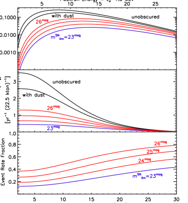
Figure 6: Upper Panel: Extreme lower bounds to the DSNB detection rate obtained by summing supernovae observed by surveys with different limiting magnitudes, the blue curve is the limiting magnitude proposed by LSST and Pan-STARRS. The blue and red curves represent a lower limit because they apply no correction for supernovae that are too dim or too obscured to be seen in surveys. The two black curves are shown for comparison: Top black curve is the DSNB flux from all core-collapse events in the universe out to redshift z $\sim$ 6. Second top black curve is the DSNB flux from core-collapse events after considering dust obscuration but with infinite survey limiting magnitude. Results assume $T_{\nu}=4$ MeV. Middle Panel: The integrated DSNB detection rate, i.e. the detection rate above a certain antineutrino energy and integrated out to $\epsilon_{\nu}$ = 30 MeV. The colors indicate the same features as in the top plot. Lower Panel: The fraction of the DSNB detection rate from the observed core-collapse events over those from the total collapse events. That is, a middle-panel red/blue curve divided by the highest black curve. Note that in this figure the x-axis starts at 2 MeV because no events can be detected below the threshold energy of 1.8 MeV.

The upper panel shows the predicted neutrino detection rate from the observed core-collapse events versus neutrino energy. Results for the neutrino detection rate from core-collapse events observed with different limiting magnitude (from $m_{\rm lim}^{\rm sn}=23^{\rm mag}-26^{\rm mag}$) are plotted. Additionally, the highest black curve plots the detection rate from all core-collapse events within the horizon (i.e., with no limiting magnitude applied) for comparison. The second highest black curve, also shows the detection rate for infinite survey limiting magnitude, but shows an estimate of the effect of dust extinction in the host galaxy. The middle panel shows the integrated neutrino detection rate $\phi_{\nu}^{\rm survey}(>\epsilon)$ above energy $\epsilon$. In other words, this is the energy-integrated version of the upper panel. The lowest panel shows the fraction of the neutrino detection rate from the observed supernovae over the events from all supernovae in the universe, that is, the corresponding middle-panel red/blue curve divided by the highest black curve.

The difference between the two black curves in Fig. 6 gives an indication of the neutrino contribution from dust-obscured supernovae. We see that an even larger effect is the loss of supernovae due to finite survey limiting magnitude. Note that when adding dust effects and limiting magnitudes, the reductions of detection rates are more severe at low neutrino energies. This is because observed neutrinos are redshifted, and as a result, a larger portion of low-energy neutrinos come from higher redshift where dust obscuration is more severe and supernova apparent magnitudes are dimmer because of larger distances.

The observability of this energy dependence is to be understood in the context of the energy threshold of the neutrino detectors. For example, Super-K in its present form can discriminate from atmospheric backgrounds, and thus detect, cosmic neutrinos in the $\sim 18-26$ MeV range. If Super-K is enhanced with gadolinium beacom03 , background rejection would be sufficiently improved in the 10 – 18 MeV range to open this crucial window onto the DSNB.

One sees more directly from the lower panel what portion of the total neutrino events detected by neutrino detector come from the observed core-collapse events with certain survey limiting magnitudes. This panel shows that $\sim 18\%$ of the neutrino events detected above 10 MeV are contributed by core-collapse events observed by surveys with a $23^{\rm mag}$ limiting magnitude.

We could thus estimate the extreme lower limit to the DSNB to be $\approx 15\%$ of the total detection events in the 10 – 18 MeV range, and $\approx 29\%$ of the total events in the 18 – 26 MeV range, assuming surveys with $m_{\rm lim}^{\rm sn}\approx 23^{\rm mag}$. Surveys including deeper scans will see larger fractions, e.g., approaching $\approx 54\%$ of the event rate within 18 – 26 MeV for $m_{\rm lim}^{\rm sn}\approx 25^{\rm mag}$. Notice that the numbers we showed above might be slightly lower than the percentages read directly from the lower panel of Fig. 6, since the numbers above are integrated only through the detectable energy range to reflect the best of what neutrino detectors would observe, while in Fig. 6, the numbers are integrated out to 30 MeV.

References

- (1) K. Hirata et al., Phys. Rev. Lett. 58, 1490 (1987).
- (2) R. M. Bionta et al., Phys. Rev. Lett. 58, 1494 (1987).
- (3) O. Kh. Guseinov, Sov. Astron. 10, 613 (1967); G. S. Bisnovatyi-Kogan and Z. F. Seidov, Sov. Astron. 26, 132 (1982); L. M. Krauss, S. L. Glashow and D. N. Schramm, Nature 310, 191 (1984); G. S. Bisnovatyi-Kogan and Z. F. Seidov, New York Academy Sciences Annals 422, 319 (1984); G. V. Domogatskii, Sov. Astron. 28, 30 (1984); A. Dar, Phys. Rev. Lett. 55, 1422 (1985); S. E. Woosley, J. R. Wilson and R. Mayle, Astrophys. J. 302, 19 (1986).
- (4) T. Totani and K. Sato, Astropart. Phys. 3, 367 (1995); R. A. Malaney, Astropart. Phys. 7, 125 (1997); D. H. Hartmann and S. E. Woosley, Astropart. Phys. 7, 137 (1997); M. Kaplinghat, G. Steigman and T. P. Walker, Phys. Rev. D 62, 043001 (2000); S. Ando, K. Sato and T. Totani, Astropart. Phys. 18, 307 (2003); M. Fukugita and M. Kawasaki, Mon. Not. Roy. Astron. Soc. 340, L7 (2003).
- (5) S. Ando and K. Sato, New J. Phys. 6, 170 (2004); F. Iocco, G. Mangano, G. Miele, G. G. Raffelt and P. D. Serpico, Astropart. Phys. 23, 303 (2005); L. E. Strigari, J. F. Beacom, T. P. Walker and P. Zhang, JCAP 0504, 017 (2005); C. Lunardini, Astropart. Phys. 26, 190 (2006); J. F. Beacom and L. E. Strigari, Phys. Rev. C 73, 035807 (2006); B. Aharmim et al. [SNO Collaboration], Astrophys. J. 653, 1545 (2006); M. Wurm, F. von Feilitzsch, M. Goeger-Neff, K. A. Hochmuth, T. M. Undagoitia, L. Oberauer and W. Potzel, Phys. Rev. D 75, 023007 (2007).
- (6) F. Daigne, K. A. Olive, P. Sandick and E. Vangioni, Phys. Rev. D 72, 103007 (2005).
- (7) L. E. Strigari, M. Kaplinghat, G. Steigman and T. P. Walker, JCAP 0403, 007 (2004) [arXiv:astro-ph/0312346].
- (8) H. Yuksel, S. Ando and J. F. Beacom, Phys. Rev. C 74, 015803 (2006) [arXiv:astro-ph/0509297].
- (9) C. Lunardini, Phys. Rev. D 75, 073022 (2007) [arXiv:astro-ph/0612701].
- (10) S. Horiuchi, J. F. Beacom and E. Dwek, Phys. Rev. D 79, 083013 (2009).
- (11) C. L. Fryer et al., Astrophys. J. 707, 193 (2009) [arXiv:0908.0701 [astro-ph.SR]].
- (12) M. Malek et al. [Super-Kamiokande Collaboration], Phys. Rev. Lett. 90, 061101 (2003) [arXiv:hep-ex/0209028].
- (13) J. F. Beacom and M. R. Vagins, Phys. Rev. Lett. 93, 171101 (2004) [arXiv:hep-ph/0309300].
- (14) G. Miknaitis et al., Astrophys. J. 666, 674 (2007) [arXiv:astro-ph/0701043].
- (15) J. A. Frieman et al., Astron. J. 135, 338 (2008) [arXiv:0708.2749 [astro-ph]], M. Sako et al., Astron. J. 135, 348 (2008) [arXiv:0708.2750 [astro-ph]].
- (16) G. Bazin et al., Astron. Astrophys. 499, 653 (2009) [arXiv:0904.1066 [astro-ph.CO]], N. Palanque-Delabrouille et al., [arXiv:0911.1629 [astro-ph.CO]],
- (17) T. Dahlen et al., Astrophys. J. 613, 189 (2004) [arXiv:astro-ph/0406547], T. Dahlen, L. Strolger, and A. G. Riess, AAS Abstracts, 215, 430.23 (2010).
- (18) S. Gezari et al., Astrophys. J. 690, 1313 (2009) [arXiv:0808.2812 [astro-ph]].
- (19) S. G. Djorgovski et al., Astronomische Nachrichten, 329, 263 (2008) [arXiv:0801.3005 [astro-ph]].
- (20) A. Rau et al., PASP. 121, 1334 (2009) [arXiv:0906.5355 [astro-ph.CO]], N. M. Law et al., PASP. 121, 1395 (2009) [arXiv:0906.5350 [astro-ph.IM]].
- (21) A. J. Drake et al., Astrophys. J. 696, 870 (2009) [arXiv:0809.1394 [astro-ph]].
- (22) A. Lien and B. D. Fields, JCAP 0901, 047 (2009) [arXiv:0902.0979 [astro-ph.CO]].
- (23) J. P. Bernstein, D. Cinabro, R. Kessler, S. Kuhlman, LSST Science Book, Version 2.0, [arXiv:0912.0201 [astro-ph.IM]].
- (24) D. Richardson, D. Branch, D. Casebeer, J. Millard, R. C. Thomas, E. Baron, Astron. J. 123, 745 (2002)
- (25) A. A. Miller et al., Astrophys. J. 690, 1303 (2009) [arXiv:0808.2193 [astro-ph]].
- (26) A. Gal-Yam et al., Nature 462, 624 (2009) [arXiv:1001.1156 [astro-ph.CO]].
- (27) R. M. Quimby et al., [arXiv:0910.0059 [astro-ph.CO]].
- (28) C. L. Fryer, Astrophys. J. 522, 413 (1999) [arXiv:astro-ph/9902315].
- (29) K. Sumiyoshi, S. Yamada and H. Suzuki, Astrophys. J. 667, 382 (2007) [arXiv:0706.3762 [astro-ph]].
- (30) K. Sumiyoshi, S. Yamada and H. Suzuki, [arXiv:0808.0384 [astro-ph]].
- (31) K. Nakazato, K. Sumiyoshi, H. Suzuki and S. Yamada, Phys. Rev. D 78, 083014 (2008) [Erratum-ibid. D 79, 069901 (2009)] [arXiv:0810.3734 [astro-ph]].
- (32) C. Lunardini, Phys. Rev. Lett. 102, 231101 (2009) [arXiv:0901.0568 [astro-ph.SR]].
- (33) A. Heger, C. L. Fryer, S. E. Woosley, N. Langer and D. H. Hartmann, Astrophys. J. 591, 288 (2003) [arXiv:astro-ph/0212469].
- (34) A. MacFadyen and S. E. Woosley, Astrophys. J. 524, 262 (1999) [arXiv:astro-ph/9810274].
- (35) E. Komatsu et al. [WMAP Collaboration], Astrophys. J. Suppl. 180, 330 (2009) [arXiv:0803.0547 [astro-ph]].
- (36) H. T. Janka, K. Langanke, A. Marek, G. Martinez-Pinedo and B. Mueller, Phys. Rept. 442, 38 (2007) [arXiv:astro-ph/0612072].
- (37) R. Buras, M. Rampp, H. T. Janka and K. Kifonidis, Astron. Astrophys. 447, 1049 (2006) [arXiv:astro-ph/0507135].
- (38) A. Mezzacappa, M. Liebendoerfer, O. E. B. Messer, W. R. Hix, F. K. Thielemann and S. W. Bruenn, Phys. Rev. Lett. 86, 1935 (2001) [arXiv:astro-ph/0005366].
- (39) T. A. Thompson, A. Burrows and P. A. Pinto, Astrophys. J. 592, 434 (2003) [arXiv:astro-ph/0211194].
- (40) H. Yuksel and J. F. Beacom, Phys. Rev. D 76, 083007 (2007) [arXiv:astro-ph/0702613].
- (41) P. Vogel and J. F. Beacom, Phys. Rev. D 60, 053003 (1999) [arXiv:hep-ph/9903554].
- (42) A. Strumia and F. Vissani, Phys. Lett. B 564, 42 (2003) [arXiv:astro-ph/0302055].
- (43) P. Madau, H. C. Ferguson, M. E. Dickinson, M. Giavalisco, C. C. Steidel and A. Fruchter, Mon. Not. Roy. Astron. Soc. 283, 1388 (1996); A. M. Hopkins, Astrophys. J. 615, 209 (2004) [Erratum-ibid. 654, 1175 (2007)] [arXiv:astro-ph/0407170]. A. M. Hopkins and J. F. Beacom, Astrophys. J. 651, 142 (2006) [arXiv:astro-ph/0601463].
- (44) C. B. D’Andrea et al., Astrophys. J. 708, 661 (2010) [arXiv:0910.5597 [astro-ph.CO]].
-
Tonry (2003)
J. Tonry, (2003), Pan-STARRS Science Goals: Supernova Science,
http://pan-starrs.ifa.hawaii.edu/project/science/precodr.html;
http://pan-starrs.ifa.hawaii.edu. - The Dark Energy Survey Collaboration (2005) The Dark Energy Survey Collaboration 2005, ArXiv e-prints, [arXiv:astro-ph/0510346]
-
The LSST Collaboration (2007)
The Large Synoptic Survey Telescope Collaboration 2007,
Science Requirements Document,
http://www.lsst.org/Science/docs/SRD.pdfLSST Science Book, Version 2.0, [arXiv:0912.0201 [astro-ph.IM]]. - Tyson (2002) J. A. Tyson and the LSST Collaboration, 2002, Proc. SPIE Int.Soc.Opt.Eng. 4836, 10
- (49) S. C. Keller et al., [arXiv:astro-ph/0702511].
- (50) D. R. Young et al., [arXiv:0807.3070 [astro-ph]].
- (51) C. Zheng et al. [SDSS-II Collaboration], Astron. J. 135, 1766 (2008) [arXiv:0802.3220 [astro-ph]].
- (52) N. Smith et al., Astrophys. J. 666, 1116 (2007) [arXiv:astro-ph/0612617]; A. J. Drake et al., [arXiv:0908.1990 [astro-ph.HE]]; A. Rest et al., [arXiv:0911.2002 [astro-ph.CO]].
- (53) J. Cooke, Astrophys. J. 677, 137 (2008), [arXiv:0711.1550 [astro-ph]].
- (54) S. Ando, Astrophys. J. 607, 20 (2004) [arXiv:astro-ph/0401531].
- (55) E. E. Salpeter, Astrophys. J. 121, 161 (1955).
- (56) C. L. Fryer, Astrophys. J. 699, 409 (2009) [arXiv:0711.0551 [astro-ph]].
- (57) C. Lunardini and O. L. G. Peres, JCAP 0808, 033 (2008) [arXiv:0805.4225 [astro-ph]].
- (58) C. S. Kochanek, J. F. Beacom, M. D. Kistler, J. L. Prieto, K. Z. Stanek, T. A. Thompson and H. Yuksel, Astrophys. J. 684, 1336 (2008) [arXiv:0802.0456 [astro-ph]].
- (59) F. Mannucci, M. Della Valle and N. Panagia, Mon. Not. Roy. Astron. Soc. 377, 1229 (2007) [arXiv:astro-ph/0702355].