Estimates of unresolved point sources contribution to WMAP 5

Abstract

We present an alternative estimate of the unresolved point source contribution to the WMAP temperature power spectrum based on current knowledge of sources from radio surveys in the $1.4-90$ GHz range. We implement a stochastic extrapolation of radio point sources in the NRAO-VLA Sky Survey (NVSS) catalog, from the original $1.4$ GHz to the $\sim 100$ GHz frequency range relevant for CMB experiments. With a bootstrap approach, we generate an ensemble of realizations that provides the probability distribution for the flux of each NVSS source at the final frequency. The predicted source counts agree with WMAP results for $S>1$ Jy and the corresponding sky maps correlate with WMAP observed maps in Q-, V- and W- bands, for sources with flux $S>0.2$ Jy. The low–frequency radio surveys found a steeper frequency dependence for sources just below the WMAP nominal threshold than the one estimated by the WMAP team. This feature is present in our simulations and translates into a shift of $0.3-0.4\sigma$ in the estimated value of the tilt of the power spectrum of scalar perturbation, $n_{s}$, as well as $\omega_{c}$. This approach demonstrates the use of external point sources datasets for CMB data analysis.

1 Introduction

Modern Cosmic Microwave Background (CMB) observations provide a powerful test of our understanding of the Universe. Within the generally accepted framework of a $\Lambda$CDM model, the 5-year measurements by the Wilkinson Microwave Anisotropy Probe (WMAP) constrain the fundamental cosmological parameters with a relative accuracy of $1-10\%$ (Dunkley et al., 2009; Komatsu et al., 2009), while the upcoming observations by the Planck satellite are expected to improve these numbers by at least a factor $\sim 3-4$ (e.g. The Planck Collaboration, 2006; Colombo et al., 2009). One of the main scientific goals of Planck, and other proposed future CMB missions (e.g. EPIC, Bock et al., 2009), is understanding the nature of Inflation. Detection of the B-mode of CMB polarization would provide direct evidence of a primordial background of Gravitational Waves arising from Inflation (Kamionkowski et al., 1997; Spergel & Zaldarriaga, 1997). Even without such detection the CMB remains the most powerful probe of Inflation currently accessible. A general prediction of inflationary models is that the fractional amplitude of density fluctuations would be nearly scale independent, so that the corresponding power spectrum could be well approximated by an Harrison-Zeldovich form $P(k)\propto k^{n_{s}}$, where the spectral index $n_{s}\simeq 1$. The amount of deviation $n_{s}-1$ constrains the shape of the inflationary potential, and current WMAP results already allow to rule out several models (Komatsu et al., 2009). Significant improvements will come from Planck and the next generation CMB missions.

However, exploitation of the full potential of CMB measurements requires a deep understanding of instrumental systematics and a careful cleaning of foreground contaminants. On small angular scales, extragalactic point sources are an important source of contamination. Bright sources, which can be detected with high significance in CMB maps, are typically accounted for by masking a small area around the source position during the estimation of the CMB angular power spectra, $C_{\ell}$. On the other hand, to a first approximation, undetected, and therefore unmasked, point sources provide a Poisson noise contribution to the measured $C_{\ell}$ as well as a non-Gaussian signature in the maps (e.g. Toffolatti et al., 1998; Pierpaoli, 2003; Pierpaoli & Perna, 2004; Serra & Cooray, 2008; Babich & Pierpaoli, 2008). An incorrect determination of this contamination can lead to relevant biases on the estimated cosmological parameters, in particular on $n_{s}$ (Huffenberger et al., 2006, 2008), whose accurate measurement depends on a careful estimate of $C_{\ell}$ over the largest range of scales probed by an experiment. In this respect the greatest expectations are now on Planck, which is a whole sky survey with a small instrumental beam and low noise level. If foregrounds and systematics are well under control, Planck will be able to confirm or falsify the WMAP findings about $n_{s}$ being significantly smaller than one. As inflation predicts that the level of departure on $n_{s}$ from one is proportional to the amount of gravitational waves expected, this also has implications on the level of B-mode polarization signal expected and is in turn relevant for the design and planning of future missions. It is therefore appropriate to try to approach the issue of point source contamination from different angles and conceive different approaches to deal with it. In this paper, we undertake this path with an application to WMAP data analysis which could lead to new approaches for point sources subtraction for Planck.

At frequencies around $\sim 1$ GHz there is a wealth of information on extragalactic sources, from nearly full-sky surveys with high angular resolution and flux sensitivity, like the Green Bank Telescope GB6 survey (Gregory et al., 1996), the NRAO-VLA Sky Survey (NVSS Condon et al., 1998) or the Faint Images of the Radio Sky (FIRST Becker et al., 2003). On the other hand, at frequencies $\sim 100$ GHz, corresponding to the optimal observational window for CMB experiments, there are only few dedicated studies covering a handful of sources. Most information comes from sources detected in CMB experiments themselves, typically representing only the bright end of the point source distribution. In addition, this lack of information limited the possibility of extrapolating data from low frequencies to the CMB “gold spot”.

To estimate the residual point sources contribution, the WMAP team assumed that unresolved sources followed the same frequency scaling as the bright sources detected in the 5 year maps. The overall normalization of the residual power spectrum was then determined by a fit to maps at three highest frequencies. This approach can be considered internal, as it takes into account (mostly) only the WMAP data itself, without relying on the low-frequency information form other available point sources surveys. As other radio surveys provide alternative and further information on radio sources properties, incorporating such results in the CMB data analysis pipeline could improve the estimation of the extragalactic sources contamination, or provide an external crosscheck of the WMAP results.

Different authors provided estimates of source counts at CMB frequencies on the basis of the physical properties of the different source populations (e.g. Toffolatti et al., 1998; de Zotti et al., 2005). However, multifrequency studies, describing the scaling of sources from middle frequencies, $\nu\sim 20$ GHz, to $\sim 100$ GHz, are now starting to appear (Sadler et al., 2008) and more are expected in the future. Together with existing studies describing sources’ behaviour from low to intermediate frequencies, these allow to predict sources contamination in CMB maps starting from the low frequency surveys. Such predictions could be used in future data analysis to make specific assessments on point sources contamination in CMB maps in real space, and account for them with techniques different from the Fourier–based ones currently used.

In this work we follow the empirical approach outlined above to assess the unresolved point sources contribution to the WMAP data and its impact on cosmological parameters. We use the NVSS catalog as a template of source fluxes and positions at radio frequency, and extrapolate that information to CMB frequencies. At difference with previous works, we extrapolate each individual source in the NVSS rather than generating source populations at CMB frequencies by randomly sampling a theoretical distribution, or by extrapolating only the statistical properties of the source population (e.g. Waldram et al., 2007). This work therefore provides a crosscheck of WMAP estimates of undetected point sources contamination, and hence of the determination of $n_{s}$ and other parameters. As mentioned above, since this approach maintains the information on the actual spatial distribution of sources, it can be useful in cleaning future Planck maps or to estimate the impact of clustering. Here, however, we refrain from using an alternative likelihood approach to the treatment of point sources in the parameter estimation and adopt the WMAP strategy to that aim.

The outline of the paper is as follow. In Section 2 we briefly review the contribution of unresolved sources to CMB temperature spectra. Section 3 describes our extrapolation procedure of NVSS source to WMAP frequencies. In section 4 and 5 we discuss the implication of our approach at the number counts and maps level, respectively, while in section 6 we debate the corresponding impact on determination of cosmological parameters. Finally, in section 7 we draw our conclusions.

2 Unresolved Sources Contribution to CMB spectra

The angular resolutions of WMAP ($\gtrsim 13$ arcmin) and Planck ($\gtrsim 5$ arcmin) are significantly larger than the angular dimensions of typical extragalactic radio sources, which can then be effectively considered as point–like objects in the resulting CMB maps. Several works studied the secondary contribution to CMB anisotropies due to point sources below the detection threshold (e.g. Franceschini et al., 1989; Tegmark & Efstathiou, 1996; Toffolatti et al., 1998; Scott & White, 1999). In this section we briefly summarize the main results.

Unresolved sources contribution to $C_{\ell}$ can be divided into a Poisson term due to the random sources positioning, and a correction accounting for clustering in the sources distribution. We consider CMB observations at a single frequency $\nu_{0}$ and suppose that all sources above a limit flux $S_{c}$ will be detected and masked from the final map, and assume a source population characterized by the differential counts $dN(>S)/dS$.

The Poisson noise contribution to the measured CMB $C_{\ell}$ is then given by:

$$C_{\ell}^{\rm src}=g^{2}(\nu_{0})\int_{0}^{S_{c}}dS\,S^{2}\,\left|\frac{dN}{dS}\right|$$ (1)

where $g(\nu)$ converts from flux density to thermodynamic temperature:

$$g(\nu)={\frac{c^{2}h^{2}}{2k^{3}T_{0}^{2}x^{2}}}{\frac{(e^{x}-1)^{2}}{x^{2}e^{x}}}~{},\,x={\frac{h\nu}{kT_{0}}}~{}.$$ (2)

The source correction does not depend on $\ell$ and, since approximately $C_{\ell}\propto\ell^{-2}$ at high multipoles up to $\ell\sim 2000$, the source correction becomes relevant on angular scales smaller than $180/\ell\sim 180/1000\sim 0.2\deg$. The correction due to clustering is given by:

$$C_{\ell}^{clust}=g^{2}(\nu_{0})\omega_{\ell}\left(\int_{0}^{S_{c}}dS\,S\,\left|\frac{dN}{dS}\right|\right)^{2}~{};$$ (3)

here $\omega_{\ell}$ is the harmonic transform of the source two-point angular correlation function.

Real CMB experiments typically have complicated noise properties, due to a combination of effects including instrumental systematics, scanning strategy and foreground removal. As a consequence, the probability of detecting a point source with flux $S_{0}$ will not be uniform on the whole sky and $S_{c}$ will not be well defined. This is not irrelevant as the unresolved point sources spectrum in eq.1 is typically dominated by the strongest amongst the residual sources. While the source population above $\gtrsim 1$ Jy in the WMAP 5 year catalog (WMAP5, Wright et al., 2009) is well described by an Euclidean scaling of the number counts $dN/dS\propto S^{-2.5}$, detected fainter sources suffers from significant completeness issues. Depending on the frequency band considered, $\gtrsim 90\%$ of detected sources have a flux $\geq 0.7$ Jy. Assuming then an optimistic detection threshold $S_{c}=0.7$ Jy and the de Zotti et al. (2005) model for $dN/dS$, we can estimate that sources with $S\lesssim 0.1$ Jy contribute $\lesssim 10\%$ of the total unresolved source power in WMAP data, as shown in figure 1. On the contrary, for Planck, whose $90\%$ detection confidence limit is expected to be $S_{c}=0.2$ Jy at 100 GHz (Vielva et al., 2003), sources with $S\sim 0.1$ Jy will play a dominant role in determination of $C_{\ell}^{src}$. Therefore, the accuracy required for the extrapolations at a given flux level depends on the characteristics of the target experiment.

Figure 1: Fraction of unresolved source contribution to WMAP spectra attributed to sources with fluxes $\leq S_{*}$, assuming that all sources with $S\geq 0.7$ Jy have been removed from the maps. We used the de Zotti et al.(2005) model for the number counts of sources with $S<0.7$ Jy. Sources below $0.1$ Jy contribute $\lesssim 10\%$ of the total unresolved power.

3 Extrapolation Procedure

3.1 Reference Catalogs

Instead of extrapolating sources directly from NVSS to WMAP frequencies, we consider a number of intermediate steps, depending on the initial flux of the source considered. This is particularly relevant at frequencies below 20 GHz, where a single power law is not an accurate description for many sources (e.g. Sadler et al., 2006). By introducing several intermediate steps, we account for the diversity of behaviours observed in the data. The number and frequency range of the steps used here was determined by available data. In selecting the reference catalogs that we will use for the extrapolation, our goal was to get a coverage of fluxes relevant for the estimation of unresolved sources contribution to WMAP data over the full range of frequencies considered. While this is not an issue in the $\sim$ GHz range, coverage becomes sketchier and patchier at higher $\nu$. According to the discussion in section 2, the main contamination to WMAP spectra is due to undetected sources with fluxes $0.1\sim 0.7$ Jy in the CMB frequency range ($40-90$ GHz). We will show this population to be dominated by sources with flat spectrum ($\alpha>-0.5$ and $S\propto\nu^{\alpha}$), therefore corresponding to sources with fluxes from a few hundreds of mJy to a few Jy at $1.4$ GHz.

In order to perform the extrapolation, we considered the following sets of measurements:

• The NRAO-VLA Sky Survey (NVSS): it covers the full sky north of $-40\deg$ declination with an angular resolution of $45^{\prime\prime}$ at $1.4$ GHz. It includes about $1.8\times 10^{6}$ discrete sources with a completeness limit of $S_{1.4}=2.5$ mJy.

• The Green Bank Telescope Survey at 6cm (GB6) observed the sky in the declination band $0\deg<\delta<75\deg$ with an angular resolution $\sim 3.5^{\prime}$ (however, the actual beam is not circular). It includes $75162$ sources above $S_{4.8}=18$mJy.

• The NVSS followup measurements by Mason et al. (2009). A set of 3165 NVSS faint sources with $S_{1.4}<100$ mJy and falling in the Cosmic Background Imager (CBI Readhead et al., 2004) field was observed at $\nu=31$ GHz using the Green Bank Telescope and the Owens Valley Radio Observatory. The resulting set of observations allowed to derive the distribution of spectral indexes $\alpha_{1.4}^{31}$ for sources with $S_{1.4}\leq 0.1$ Jy.

• The Ninth Cambridge Survey at 15 GHz (9C) followup observations by Waldram et al. (2007). The catalog includes 121 sources selected at $15.2$ GHz with a completeness limit of $S_{15}=25$ mJy and simultaneous measurements at $4.85$, $15.2$, $22$ and $43$ GHz. As the 9C survey covers the sky area observed by the Very Small Array (VSA Watson et al., 2003), which was selected to be devoid of bright sources, the sample contains only a handful of sources with $S>100$ mJy.

• The AT20G followup observations by Sadler et al. (2008). The work presents two samples of sources selected at $20$ GHz with simultaneous measurements at $90$ GHz: a first set of 59 inverted spectra sources with $S_{20}>50$ mJy, and a flux-limited sample comprising 70 sources with $S_{20}>150$ mJy. We consider here only the flux-limited sample, which constitutes our main reference sample for the extrapolation of sources with $S_{20}\leq 1$ Jy from 20 to 94 GHz.

• At frequencies above $\sim 23$ GHz and for fluxes above $\sim 1$ Jy, the most comprehensive survey of point sources is provided by the WMAP 5 year catalog. WMAP observed the sky at five broad bands K, Ka, Q, V and W with central frequencies of $\sim 23,33,41,61,94$ GHz respectively. The catalog includes a total of 390 sources which have been detected with a $5\sigma$ confidence level in at least one of the bands, and is complete for fluxes above $\sim 1$ Jy in all bands.

3.2 Method

Since the number of sources with high frequency information is smaller than the number of NVSS sources, reconstructing the actual scaling of individual sources is not possible. Our assumption is thus that from the reference catalogs discussed above, we can build reference samples which are representative of the behaviour of the whole source population in the respective range of frequencies and fluxes. We then perform a set of bootstrap simulations in which at each extrapolation step, a simulated source is randomly paired to a reference source in the catalog covering the next higher frequency range considered, and we use the measured spectral index of the reference source to further extrapolate the simulated source. Some of the catalogs considered provide multifrequency information for their sources. When this is the case, we use the set of spectral indexes of the catalog source to extrapolate fluxes over the range of frequencies considered. For each source in the NVSS catalog, we generate a set of 800 simulations. While in two different simulations a given source can be extrapolated in different ways, the set of simulations provides the probability distribution for flux at WMAP frequencies.

In broad terms, we define two main frequency ranges: 1) the interval from NVSS to the lowest WMAP band, $1.4-23$ GHz, and 2) the WMAP frequency range, $23-94$ GHz. Sources with $S_{1.4}\leq 100$ mJy are extrapolated directly to 23 GHz according to Mason et al. (2009), while for those with $S_{1.4}\geq 300$ mJy we introduce a number of intermediate steps based based on the GB6 and Waldram et al. (2007) measurements. In the intermediate flux range, we weight the two approaches in order to fit the 33 GHz low flux counts. From 23 GHz upwards, sources with $S_{23}>1$ Jy are propagated based on the WMAP5 catalog, while for lower flux sources we base the extrapolation on the Sadler et al. (2008) and Waldram et al. (2007) reference samples.

In the following, we discuss each step in detail:

• The 1.4 GHz to 4.85 GHz reference sample. Kimball & Ivezić (2008) provide a unified catalog of sources from four radio surveys NVSS, GB6, FIRST, WENS and from the optical SDSS surveys, matching sources in the different catalogs. From the NVSS-GB6 pairings identified in that work, we construct a reference sample of sources which provides spectral indexes between $1.4$ GHz and $4.85$ GHz. We consider only pairs in which the GB6 counterpart is found within $70^{\prime\prime}$ of the NVSS source, corresponding to an estimated completeness of $0.979$ and an efficiency (fraction of detected pairs corresponding to actual physical matches) of $0.79$ (for further details see Kimball & Ivezić, 2008). In addition, we exclude sources flagged as extended in the GB6 survey and include only unique pair of sources, i.e. sources in one catalog with multiple matches in the other catalog are excluded. Since multiple sidelobes of a single source may show up as different NVSS components, in this way we may bias the pairs toward compact sources. However NVSS resolution is such that less than $1\%$ of sources is resolved into multiple components (Best et al., 2005), compared with $\sim 7\%$ of GB6 sources with multiple NVSS matches in the reference catalog. We then conclude that the majority of multiple matches we find are spurious pairs.

  The distribution of spectral indexes so obtained describes the $1.4-4.85$ GHz behaviour of sources selected at the GB6 frequency, and can be used to accurately propagate sources from $4.85$ GHz to the lower frequency. In order to use this distribution to extrapolate from $1.4$ GHz to higher frequencies, some adjustments are required. The NVSS survey has a flux limit of $2.5$mJy, while the GB6 includes sources above $18$mJy, therefore low–flux NVSS sources which appear also in the GB6 survey will be biased to have a rising spectral index. Figure 2 shows the average $\alpha_{1.4}^{4.8}$ as a function of $S_{1.4}$. While for $S_{1.4}\gtrsim 0.3$ Jy the spectral index is a decreasing function of the NVSS flux, for $S_{1.4}\lesssim 0.1$ Jy $\alpha_{1.4}^{4.8}$ shows a steep upturn due to completeness issues. We therefore exclude from the reference sample all sources with $S_{1.4}\leq 0.1$ Jy. We further divide the reference sample in 10 logarithmic bins covering the flux range $0.1-3.0$ Jy, depending on the value of $S_{1.4}$, with an additional bin including all sources with $S_{1.4}>3$ Jy. In the end the reference sample includes  31000 sources, with corresponding spectral index $\alpha_{i}$ and uncertainty $\delta\alpha_{i}$.

  

  Figure 2: The average $1.4-4.85$ GHz spectral index of GB6 sources as a function of $1.4$ GHz flux. Below $S_{1.4}\sim 100$mJy NVSS sources with a GB6 counterpart are biased to have upturn spectra.

  In principle, since the reference sample is based on sources with matches in both NVSS and GB6 catalogs, we may be missing: a) sources with strongly rising spectra, which are absent in NVSS but are detected by GB6, or b) sources with very steep spectra, which fall below the GB6 detection threshold. Waldram et al. (2009) find that $4.3\%$ of sources selected at $15.2$ GHz with $10{\rm mJy}\leq S_{15}\leq 15$mJy do not have an NVSS counterpart. GB6 sources are selected with higher threshold (18mJy) and at lower frequencies than Waldram et al. (2009). Therefore, sources of type (a) would require spectral indexes significantly more rising than those of the rising population discussed in that work, an we expect the fraction of sources detected at $4.85$ GHz but not in the NVSS to be significantly lower than Waldram et al. (2009) estimates. Regarding point (b), we note that sources in the reference sample with $100\leq S_{1.4}\leq 200$ mJy have an average spectral index $\alpha_{1.4}^{4.8}=-0.84\pm 0.34$. Therefore we estimate the fraction of NVSS sources with no GB6 counterpart to be $\sim 5\%$ at $100$mJy and $\sim 0.5\%$ at $150$ mJy.

• From 1.4 GHz to 23 GHz for sources with $S_{1.4}\geq 300$ mJy. From the previous discussion, we conclude that the thinned reference sample defined above provide an accurate description of the frequency scaling from 1.4 to 4.85 GHz for the population of sources with $S_{1.4}\gtrsim 300$ mJy, which are responsible for the bulk of source contamination at CMB frequencies. Therefore, each NVSS source with $S_{1.4}>300$ mJy is randomly paired to a spectral index $\alpha_{i}$ from the corresponding flux bin of the thinned reference sample. We then randomly draw a spectral index $\bar{\alpha}$ from a Gaussian with mean $\alpha_{i}$ and width $\delta\alpha_{i}$. In this way we incorporate in the extrapolation the measured uncertainty on $\alpha_{i}$, however, since the distribution of the reference spectral indexes is not necessarily Gaussian, the overall distribution of the $\bar{\alpha}$ both within a single realization and among different realizations will not be Gaussian. The flux of the NVSS source is extrapolated to $4.85$ GHz assuming $S\propto\nu^{\bar{\alpha}}$. The source is then propagated to $23$ GHz using the spectral indexes by Waldram et al. (2007). Since the flux threshold of the $15.2$ GHz sample is higher than the GB6 limit, we need to thin the catalog to avoid that sources with low fluxes at $4.85$ will bias the sample toward flatter spectral indexes. Due to the low number of sources, we cannot study the behaviour of $\alpha(S)$ as done in the previous section. Instead we compute the average spectral index $\alpha_{4.8}^{15}$ using all the 121 sources in the sample. Using this average $\alpha_{4.8}^{15}$, we extrapolate the $15.2$ GHz threshold to $4.85$ GHz and remove form the $4.8-15.2$ GHz reference sample all sources with $S_{4.8}$ below this value. The process is iterated until no more sources are rejected. We are left with $76$ sources with $S_{4.85}>75$ mJy, which we assume provide a representative description of the behaviour of sources between $4.85$ and $23$ GHz. Each source simulated at the previous step is paired with a random source in this new reference sample, and its corresponding set of spectral index. We use this set to propagate the source to $23$ GHz, going through an intermediate step at $15.2$ GHz.

• From 1.4 GHz to 23 GHz for sources with $S_{1.4}\leq 100$ mJy. For low flux sources, $S_{1.4}<100$ mJy, we extrapolate directly to $23$ GHz assuming $S\propto\nu^{\alpha}$, with $\alpha$ randomly drawn from the distribution of spectral indexes by Mason et al. (2009). In order to be consistent with the treatment of sources with $S_{1.4}>100$ mJy described above, we assumed that such distribution be valid in the range $1.4-23$ GHz, even if it is based on $31$ GHz followup of NVSS sources.

• From 1.4 GHz to 23 GHz for sources with $100{\rm mJy}<S_{1.4}<300$ mJy. Sources with $100{\rm mJy}<S_{1.4}<300$ mJy are above the upper validity limit of the Mason et al. (2009) study, and may yet be slightly affected by spurious effects in the NVSS - GB6 reference sample defined above. Therefore, in this intermediate regime, we randomly chose between the two approaches discussed above, and tune the selection function to reproduce low flux counts at higher frequencies. The probability of extrapolating sources using the spectral index distribution of Mason et al. (2009) is given by:

  $$P(S_{1.4})=\frac{1}{2}\left[1-\tanh\left(\frac{S_{1.4}-S_{*}}{\Delta}\right)\right]~{}.$$ (4)

  The values $S_{*}$ and $\Delta$ are chosen by fitting the $33$ GHz number counts from the extrapolation procedure described here to the observed number counts by DASI and VSA in the $0.05-1$ Jy range. Sources with lower fluxes are not a significant contaminant in WMAP maps, as discussed above. Note that we do not require the selection function in equation 4 to be continuous at the $100$mJy and $300$mJy boundaries.

• From 23 GHz to 94 GHz for sources with $S_{23}\geq 1$ Jy. Sources with $S_{23}>1$ Jy are extrapolated to higher frequencies according to the WMAP5 catalog itself. We divide the WMAP5 catalog in two sub catalogs comprising sources with $S_{23}>2$ Jy and $1{\rm Jy}<S_{23}<2$ Jy, respectively containing $69$ and $166$ elements. When a simulated source has $S_{23}>1$ Jy, we randomly pair it with a spectral index from the subcatalog covering the corresponding flux range, and extrapolate the source to higher frequency using a simple power law.

• From 23 GHz to 94 GHz for sources with $S_{23}<1$ Jy. For fluxes below $\sim 1$ Jy the WMAP catalog is not complete. Waldram et al. (2007) suggest a procedure to extrapolate fluxes into the WMAP frequency range based on the spectral behaviour of the source around $\sim 20$ GHz. For sources for which $\alpha_{22}^{43}\leq\alpha_{15}^{22}\leq 0$ they suggest fitting a quadratic form to the $\log(S)-\log(\nu)$ relation, while for the remaining sources they adopt a linear $\log(S)-\log(\nu)$, using $\alpha_{22}^{43}$. Alternatively, we consider the set of spectral indexes based on the Sadler et al. (2008) sample. Taking into account both sets of observations, we consider then the following extrapolation strategy for sources with $S_{23}<1$ Jy:

  • Sources with $S_{23}<100$ mJy are randomly paired to source of Waldram et al. (2007) and extrapolated according to the procedure described there;

  • Sources with $S_{23}>400$mJy are propagated assuming a single power law with spectra index drawn randomly from the reference sample of Sadler et al. (2008);

  • Sources with $100<S_{23}<400$mJy are extrapolated choosing randomly between the previous two methods; the probability of selecting one method over the other is given by the relative number of sources in the relevant flux range.

In addition, when at a given step we have different extrapolation procedures depending of the flux of the source, we do not switch abruptly from one regime to the other, but we adopt a linear transition between the two with a width which is the greater of $100$mJy and $10\%$ of the threshold flux. Moreover, we do not consider polarization.

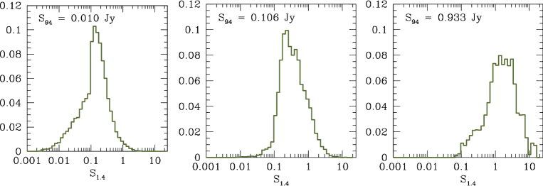
Figure 3: Distributions of the initial 1.4 GHz fluxes for sources with a final 94 GHz as indicated in the respective panels. Histograms refer to the full set of 800 simulations and have been normalized to have unit area.

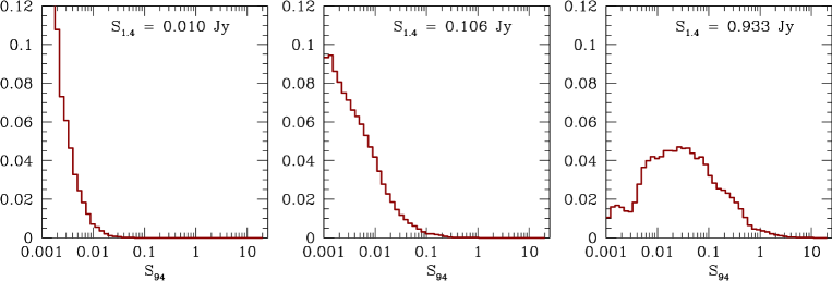
Figure 4: As in figure 3 but showing distributions of simulated 94 GHz fluxes for sources with initial 1.4 GHz flux as indicated in the different panels.

4 Results

4.1 Flux distribution

This approach provides both the probability that a source with an NVSS flux $S_{1.4}$ will have a 94 GHz flux $S_{94}$, i.e. $P(S_{94}|S_{1.4})$, as well as the complementary distribution $P(S_{1.4}|S_{94})$. In figure 3 we plot the distribution of the initial 1.4 GHz fluxes for sources with final 94 GHz fluxes of $S_{94}\sim 0.01,\sim 0.10$ and $\sim 1.0$ Jy, which provides an estimate of $P(S_{1.4}|S_{94})$. The plots refer to the full set of 800 simulations. Figure 4 shows instead $P(S_{94}|S_{1.4})$. A general expectation is that for flux levels relevant to CMB experiments, the high frequency population of sources is dominated by objects with flat spectral indexes. We recover this behaviour in the simulations, as shown in figures 3 and 4. In particular, according to the discussion of section 2, the residual contamination in WMAP maps will be dominated by sources with $S\gtrsim 0.1$ Jy in the frequency range $60-90$ GHz, and we expect the majority of these sources to have $S_{1.4}\gtrsim 100$mJy. Inaccuracy in the extrapolations of sources with lower $S_{1.4}$ will have a minimal impact on estimates of the residual contamination in WMAP maps.

4.2 Number counts

For each simulation, we compute the corresponding differential number counts $dn(S)/dS$ and then average over the whole set of simulations. In figure 5 we compare the incomplete counts from WMAP5 source catalog with the ensemble average differential counts at the frequencies of $33,41,61$ and $94$ GHz, approximately corresponding to the central frequencies of WMAP Ka, Q, V and W bands. At 33 GHz we compare our estimation also with results from CBI, VSA, and DASI surveys, while at 94 GHz we also plot prediction from earlier works  (de Zotti et al., 2005; Waldram et al., 2007).

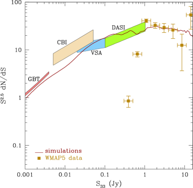
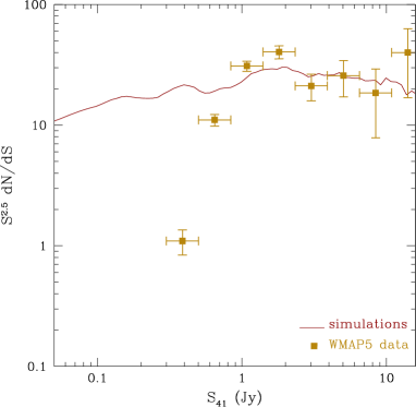
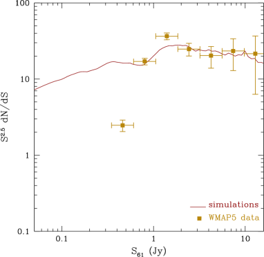
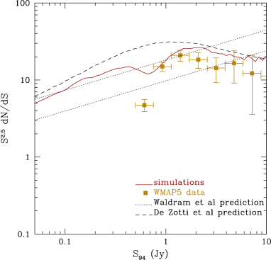
Figure 5: Comparison of the predicted Euclidean counts from the ensemble of NVSS simulations of this work (solid lines) with the incomplete counts from the WMAP 5 year catalog (squares), at the frequencies of 33, 41, 61 and 94 GHz. At 33 GHz we also plot data from the CBI, VSA and DASI survey, while at 94 GHz we compare with predictions from earlier works.

Comparison with lower flux data at $33$ GHz, shows that the methods discussed here tends to underestimate source counts below $S\sim 0.02-0.03$ Jy. These sources do not provide a relevant contribution to the total residual contamination to WMAP spectra, but will play a more relevant role for Planck data analysis. Since the uncertainty in our methods is dominated mostly by the low number of reference sources above $4.85$ GHz, we expect a better agreement as the pool of reference sources increases. In the range $0.5-1.0$ Jy, simulations show evident artifacts due to the transition between different regimes of flux extrapolation, i.e. using spectral index from the WMAP5 catalog for $S_{23}>1$ Jy. They are due to the low number of sources in that flux range in the base catalogs; as above, we expect these artifact to significantly decrease as more data over the relevant frequency and flux range will be included in the reference catalogs.

While our extrapolations correctly recover WMAP5 results at lower frequencies, counts at 94 GHz are overestimated by $\sim 50\%$. In figure 6 we plot the integrated counts $N(>S=1{\rm Jy})$ from our simulations and from WMAP5 data. For reference, we also show an analytic estimate of the counts assuming $dN/dS\propto S^{-2.5}$ and $S\propto\nu^{-0.09}$ (Wright et al., 2009), normalized to fit WMAP5 counts in K, Ka and Q bands. WMAP5 data show a steepening of the counts in W band compared to lower frequencies, while our counts seem to be in better agreement with a linear $\log(S)-\log(\nu)$ relation. As discussed in section 3.2, our extrapolations of sources with $S_{23}>1$ Jy is mainly based on the family of spectral indexes provided by the WMAP5 team, which can be approximated by a Gaussian distribution with mean $\alpha=-0.09$ and dispersion $\sigma_{\alpha}=0.17$. Therefore, as expected source counts in the simulations are in agreement with the analytic estimate plotted in figure 6; the slightly steeper behaviour seen in simulations is compatible with the actual distribution of WMAP5 spectral indexes having a tail toward steeper $\alpha$. This suggests that there is some tension between the WMAP5 W-band counts and their spectral index distribution. A possible explanation could be a progressive steepening of the spectral index of bright sources with increasing frequency. González-Nuevo et al. (2008) noticed that the spectral index of WMAP sources in the $41-64$ GHz range is steeper than their spectral index in the $5-23$GHz range, and radio source measurements in the $\sim 100-250$ GHz range by the QUaD telescope (Friedman et al., 2009) and the South Pole Telescope (SPT, Vieira et al., 2009) provide additional evidence in this direction (see de Zotti et al., 2009, for a recent review). If this is actually the case, describing the source behaviour in the $23-94$ GHz range with a single power law may not be entirely accurate.

Alternatively, there may be some unaccounted for systematics affecting WMAP detection efficiency in W band. The WMAP team required that for a source to be included in the catalog it needed to be detected at more than $5\sigma$, in at least one band. Its flux in the other bands would be included if: a) it was measured at more than $2\sigma$, b) the fitted source width is within a factor of 2 of the actual beam (Wright et al., 2009). Sawangwit & Shanks (2009) pointed out that the W band beam response to discrete sources appears to depend in a non-linear fashion on source flux. In particular, they find that the effective beam profile is significantly wider for point sources than for the Jupiter observations used as a basis for the WMAP team’s beam analysis, which can create a significant bias in determining if a source fits requirement (b). Since number counts from simulations do not include systematics due to WMAP actual detection procedure, this effect, if confirmed, could be an alternative explanation for the discrepancies between simulated and actual number counts. Further data on source behaviour at high frequency, e.g. from Planck, will help solve this issue.

In addition, all WMAP sources with measured W band flux have been detected also in at least one of the lower frequencies. As long as a WMAP source is detected in at least one band, it is masked in the power spectrum analysis (Nolta et al., 2009), and we follow the same procedure in building sky mask for the analysis of section 6. Therefore, any mismatch in the number of W band bright sources between simulations and real data will not impact our estimates of the unresolved source power as long as counts at the lower frequency for the simulations are in good agreement with WMAP findings.

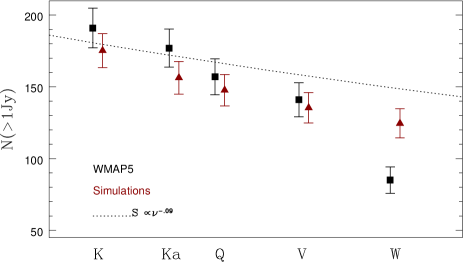
Figure 6: Comparison of integrated counts in simulations (red/triangles) and in WMAP 5 year catalog (black/squares). The dashed line shows the expected behaviour assuming a scaling of differential counts $dn/dS\propto S^{-2.5}$ and a frequency dependence $S\propto\nu^{-0.09}$. The curve amplitude is fixed by a fit to WMAP count in K, Ka and Q bands. In computing the number counts we excluded the sky area with declination $\leq-40\deg$ and within the WMAP 5yr point source catalog mask.

5 Maps

An advantage of this approach consists in that it naturally provides an estimates of bright sources position and accounts for clustering of unresolved sources. However, agreement of number counts estimated from simulations with those computed by data does not guarantee that the method correctly recovers the spatial distribution of sources. In order to check whether the simulations match the structure observed in WMAP maps, for each realization we produce source-only (i.e. without noise and CMB) maps and compare them with WMAP observed maps. Source maps also allow and independent determination of unresolved source contamination. Since WMAP estimate of this contribution is based on the Q, V and W bands data, we generate map for each of the above frequencies.

We place the sources on an HEALPIX(Górski et al., 2005) map at a resolution ${\rm N}_{\rm side}=2048$, corresponding to a pixel size of $\sim 1.7^{\prime}$. This value is considerably greater than the NVSS beam and angular resolution, so we can consider the sources as points when placing them on the map, and considerably smaller than WMAP W beam of $\sim 13^{\prime}$, so that any artifacts due to pixelization, smoothing etc. will be minimal. The actual WMAP beams are not Gaussian, their exact profile varying between each set of Differential Arrays (DAs). To reduce the number of maps we have to deal with, we consider individual frequencies, rather than individual DAs. Each map is then smoothed with an effective beam given by the average, in harmonic space, of the beam profiles of the DAs of the corresponding frequency. The smoothed maps are then degraded to a resolution ${\rm N}_{\rm side}=512$.

In order to check that our predictions recover the point source structure seen in the maps, we compute the linear correlation coefficient between each individual simulation and the corresponding WMAP 5yr map:

$$r=\frac{\langle\left({\bf X}_{i}-\langle{\bf X}\rangle\right)\,\left({\bf M}_{i}-\langle{\bf M}\rangle\right)\rangle_{S>S_{c}}}{\sigma_{\bf X}\,\sigma_{\bf M}}~{}.$$ (5)

Here ${\bf X}$ and ${\bf M}$ respectively refer to the simulated and WMAP maps, after application of an harmonic space filter $b_{\ell}/(b_{\ell}^{2}C_{\ell}+C_{\ell}^{\rm noise})$, where $b_{\ell}$ is the harmonic transform of the beam profile, $C_{\ell}$ is a theory CMB power spectrum based on WMAP5 best fit parameters (Dunkley et al., 2009) and $C_{\ell}^{\rm noise}$ is the noise power spectrum (Wright et al., 2009). The means and variances of the maps, $\langle{\bf X}\rangle$ and $\sigma_{\bf X}$, and the correlation coefficients are computed using only pixels within radius equal to the nominal frequency FWHM, of sources with flux above a threshold $S_{c}$. To assess the significance of this result, we compare the value of $r$ computed from the simulations-WMAP5 correlations, with that computed by correlating our simulations with a mock microwave sky which includes contribution from CMB, WMAP5-like noise, Galactic foregrounds and a point sources population obtained according to the procedure described in this work. In practice, we randomly chose one of the simulations as the actual distribution of point sources, and add to this a CMB realization, an anisotropic Gaussian noise term and a foreground contribution. The pixel noise variance is given by $n=n_{0}/\sqrt{N_{\rm obs}}$, where $N_{\rm obs}$ is the effective number of observations in each pixel and $n_{0}=2.197$ mK for the Q band and $6.547$ mK in W band (Limon et al., 2009). However, we do not account for noise correlations between different pixels. The foreground contribution is based on the Maximum Entropy Method maps (Gold et al., 2009). The maps are provided at a resolution $N_{\rm side}=128$ and smoothed with a $1\deg$ beam, and are thus have no power at scales $\ell\gtrsim 300$. Therefore the foregrounds contribution to the variance and mean of the mock sky, in particular to the small scales relevant to point sources, will be significantly lower than the impact on the actual WMAP sky maps. We generate different sets of mock skies, corresponding to different point sources, CMB and noise realizations. The mock sky then constitute a best case scenario, in which the point source distribution follows exactly the model discussed in this work, and several systematic effects, like foregrounds and correlated noise, are absent or play a reduced role. Tables 1 and 2 show results of the comparison in Q and W bands, respectively.

$S_{c}$ (Jy) WMAP5 mock mock mock mock mock mock maps data 1 data 2 data 3 data 4 data 5 data 6 1.0 $0.22\pm 0.07$ $0.34\pm 0.08$ $0.36\pm 0.07$ $0.37\pm 0.08$ $0.35\pm 0.07$ $0.32\pm 0.07$ $0.37\pm 0.07$ 0.5 $0.18\pm 0.05$ $0.30\pm 0.06$ $0.32\pm 0.05$ $0.31\pm 0.06$ $0.29\pm 0.05$ $0.26\pm 0.05$ $0.31\pm 0.05$ 0.2 $0.13\pm 0.04$ $0.23\pm 0.04$ $0.25\pm 0.04$ $0.23\pm 0.04$ $0.22\pm 0.04$ $0.19\pm 0.03$ $0.25\pm 0.04$ 0.0 $0.03\pm 0.02$ $0.06\pm 0.02$ $0.07\pm 0.01$ $0.06\pm 0.01$ $0.06\pm 0.01$ $0.05\pm 0.01$ $0.08\pm 0.01$

Table 1: Linear correlation coefficient $r$ between simulated source maps at $41$ GHz and WMAP 5 year Q band maps, for different flux cuts $S_{c}$. Only pixels within 1FWHM radius of sources with $S>S_{c}$ are included in the computation of $r$. For comparisons, columns 3-8 show the same quantity computed by correlating our set of simulations with mock WMAP-like skies for which the point source component follows the same distribution as our simulations.

$S_{c}$ (Jy) WMAP5 mock mock mock mock mock mock maps data 1 data 2 data 3 data 4 data 5 data 6 1.0 $0.14\pm 0.08$ $0.21\pm 0.09$ $0.24\pm 0.08$ $0.20\pm 0.08$ $0.18\pm 0.07$ $0.16\pm 0.07$ $0.18\pm 0.07$ 0.5 $0.14\pm 0.06$ $0.18\pm 0.07$ $0.21\pm 0.06$ $0.16\pm 0.06$ $0.15\pm 0.05$ $0.14\pm 0.05$ $0.15\pm 0.05$ 0.2 $0.12\pm 0.04$ $0.13\pm 0.04$ $0.16\pm 0.04$ $0.11\pm 0.03$ $0.11\pm 0.03$ $0.11\pm 0.03$ $0.11\pm 0.03$ 0.0 $0.014\pm 0.003$ $0.011\pm 0.003$ $0.014\pm 0.003$ $0.010\pm 0.002$ $0.010\pm 0.002$ $0.010\pm 0.003$ $0.011\pm 0.002$

Table 2: As table 1 but for W band.

A general remark is that even in the best case scenario we expect only a moderate level of correlation: $r\lesssim 0.40$ and $r\lesssim 0.25$ for bright sources, respectively in Q and W band. As expected, the degree of correlation between simulations and actual maps is lower than that between simulations and mock data. While for W band the difference is within the associated standard deviation, in Q band the discrepancy is of order $2\sigma$ for bright sources increasing to $\sim 3\sigma$ for faint ones. Foreground contamination is more relevant at $41$ GHz than at $94$ GHz and this may account for the significant loss of correlation in Q band.

6 Power spectra and effect on parameters

The WMAP team estimated the amplitude of the unresolved point source contribution to a cross spectrum $C_{\ell}^{Y_{1}Y_{2}}$ ($Y_{1}Y_{2}$ represents a pair of different DAs, e.g. $Q_{1}Q_{2}$, $Q_{1}V_{1}$) assuming a power-law scaling in frequency:

$$C_{\ell}^{\rm src}=A_{0}g(\nu_{1})g(\nu_{2})\left(\frac{\nu_{1}}{\nu_{Q}}\right)^{\alpha}\left(\frac{\nu_{2}}{\nu_{Q}}\right)^{\alpha},$$ (6)

where $\nu_{1},\nu_{2}$ are the frequencies of the DAs considered, $g(\nu)$ was defined in equation 2, and the spectral index $\alpha$ is assumed to be either 0, as most sources are expected to have a flat spectrum, or -0.09, corresponding to the mean of of a Gaussian fit to the spectral indexes of the actual WMAP5 catalog (Wright et al., 2009). The common amplitude $A_{0}=0.011\pm 0.001\,\mu{\rm K}^{2}{\rm sr}$ is determined by fitting the spectral shape of equation 6, to the cross spectra from the Q,V,W bands; the estimated $A_{0}$ has only a small dependence on the two values of $\alpha$ considered (Nolta et al., 2009). The final power spectrum, instead, is a linear combination of the possible VV,VW, and WW cross spectra, weighted by the corresponding inverse covariance matrix (Hinshaw et al., 2003; Nolta et al., 2009). This method is internal, as it includes information only from WMAP own measurements. On the contrary, the approach discussed in this paper, provides a partially external method, in the sense that it incorporates both information from WMAP data (to propagate sources with $S_{23}>1$ Jy) and from other surveys, and could provide a cross check of WMAP results.

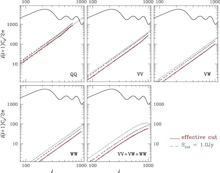
Figure 7: Estimates of the unresolved point sources contribution to CMB power spectra at different WMAP frequencies when applying the masking procedure described in the text (solid lines) or simply removing all sources with Q band flux $S_{41}>1Jy$ (dashed lines). The dotted lines show a Poisson spectrum with normalization $C_{\ell}^{src}\propto A_{0}\nu_{1}^{\alpha}\nu_{2}^{\alpha}$ with $A_{0}=0.011$ and $\alpha=-0.09$. The final power WMAP power spectrum is a combination of VV, VW and WW cross spectra and does not depend on QQ data. For reference we also show the CMB temperature power spectrum for the best fit WMAP5 cosmological model.

To estimate the unresolved point sources contamination from our simulations we need to define an individual mask for each realization. We start by applying the same Galactic cut as for the KQ85 mask, used in the WMAP5 power spectrum analysis (Nolta et al., 2009), and also mask the area outside of the NVSS sky coverage. This base mask is the same for all realizations. In addition, the KQ85 mask removes the sky area within $0.6\deg$ of sources in the WMAP5 catalog. The WMAP detection efficiency for radio sources depends on a number of factors, including frequency, position on the sky and the actual CMB and noise fluctuations around the source. Replicating all these effects in all our simulations would be too time consuming and instead we adopt a simplified procedure to “detect” and mask sources. The WMAP5 catalog is complete for sources $\gtrsim 1$ Jy at all frequencies, and the number counts for those sources follow an Euclidean distribution. Therefore, at each frequency we assume a power law shape for the number counts $F_{\nu}S^{-2.5}$, and fix the value of $F_{\nu}$ by fitting to the observed WMAP5 differential number counts ${\bar{n}}_{\nu}(S)$ for $S>1$ Jy at the appropriate frequency. We then assign to each simulated source a detection probability $P(S_{*})={\bar{n}}_{\nu}(S_{*})/(F_{\nu}S_{*}^{-2.5})$. On average, in each simulation we detect $304\pm 16$ sources, compared with 321 actual WMAP5 sources in the same sky area, and we mask a $0.6\deg$ radius around each detected source. Alternatively, we consider the conservative approach of masking only sources with a Q band flux $S_{41}>1.0$ Jy.

We apply the resulting mask to the corresponding set of maps and compute the QQ, VV, VW and WW spectra using a MASTER approach (Hivon et al., 2002). The VV, VW and WW spectra are then combined according to Hinshaw et al. (2003); notice that we only include the diagonal terms of the covariance matrix. The final estimate of the unresolved sources contribution is the average of the spectra from the individual realizations.

In figure 7 we compare our estimates with WMAP results. While our predictions are in good agreement with WMAP5 yr estimates for the QQ spectra, they show a steeper frequency behaviour. In particular, for the final combined power spectrum, we predict a residual point source contribution $\sim 50\%$ lower than WMAP estimates for the source detection strategy discussed above, and $\sim 25\%$ lower if we only mask sources with $S_{41}>1Jy$. Uncertainty on simulations results is $\sim 10\%$, comparable to the error on $A_{0}$. Notice that in figure 7 we do not plot our estimates of residual sources contamination at $\ell>700$ for the Q band, as the uncertainty in the beam asymmetries for that channel introduce significant artifacts at $\ell\gtrsim 500$ (Hill et al., 2009). Since we do not use the Q band data to estimate the point sources contribution to the final spectra, these artifacts do not alter the following discussion.

The differences between our prediction and WMAP5 estimates arise from a combination of factors. As discussed above, the reference catalog we use to extrapolate high flux sources from $20$ GHz to $94$ GHz was given by the subsample of WMAP5 sources with with fluxes $S_{23}>1$ Jy, corresponding to the approximate completeness limit of WMAP 5yr catalog. WMAP sources with $S_{23}>1$ Jy have an average spectral index ${\bar{\alpha}}=-0.21\pm 0.30$, while for sources with $S_{23}<1$ Jy ${\bar{\alpha}}=-0.09\pm 0.66$. The spectral index used by the WMAP team in order to derive the amplitude is the mean of a Gaussian fit to the spectral index distribution of all their detected sources, and is therefore affected by the shallower spectral indexes of sources with $S_{23}<1$ Jy. Note that we did not use the latter set of sources for the simulations, as for this range of fluxes and frequencies we adopted the results of Sadler et al. (2008). These results suggest that sources with fluxes in the $0.2-1$ Jy range have an average spectral index ${\bar{\alpha}}=-0.43\pm 0.31$, while for the subset of 8 sources with $S_{20}>0.8$ Jy, ${\bar{\alpha}}=-0.26\pm 0.16$, in good agreement with estimates for WMAP sources with $S_{23}>1$ Jy. Our simulations reflect this finding. As more information on the spectral behaviour of sources with K band flux in the $0.5-1.5$ Jy will become available, it will be possible to better establish if the low flux sources of WMAP catalog are biasing the estimates of the spectral index used for estimating the unresolved point sources contribution.

In addition, WMAP fix the amplitude of the unresolved source contribution $A_{0}$ by a simultaneous fit to the ensemble of cross spectra obtained using Q, V and W bands, assuming a constant frequency scaling across the corresponding range of frequencies, 41 - 94 GHz. Therefore, although the final CMB power spectra are a combination of only V and W measurements, the estimated unresolved sources contribution to such spectra depends also on Q data. In this work, instead, we estimate the point source contamination at a given frequency directly from the point sources maps at that frequency, without including information from other bands. In particular, our prediction for the final combined VV+VW+WW spectrum does not depend on 41 GHz data. As discussed in Nolta et al. (2009), the WMAP5 estimated value of $A_{0}$ using only V and W data is $\sim 10\%-40\%$ (depending on the choice of Galactic mask) lower than when using Q,V and W data, although the uncertainty in the former case is $\sim 3$ times the uncertainty in the latter. Therefore, using information from Q band may lead to a slight overestimate of $A_{0}$ at $60-90$ GHz.

As pointed out by Huffenberger et al. (2006, 2008) the point sources correction and the way it is treated in the likelihood function affects the determination of the cosmological parameters, in particular of the slope of the power spectrum of scalar perturbations, $n_{s}$. To test the effect, if any, of our approach on parameter estimation, we use COSMOMC (Lewis & Bridle, 2002) + PICO (Fendt & Wandelt, 2007) to run a set of Monte-Carlo Markov Chains (MCMC) replacing the source correction term in WMAP5 likelihood code with our results. However, we did not change the shape of the likelihood function as suggested by Huffenberger et al. (2008). We consider the six base $\Lambda$CDM parameters: physical baryon, $\omega_{b}$, and cold dark matter, $\omega_{c}$, densities; optical depth to reionization, $\tau_{e}$; tilt, $n_{s}$, and amplitude, $A_{s}$ of the power spectrum of scalar density fluctuations; the angle subtended by the sound horizon at recombination, $\theta$. We include marginalization over the amplitude of the Sunayev-Zeldovich effect and lensing. As expected, since changing the source correction effectively alters the shape of the second and third acoustic peaks in the measured spectrum, we find that $\tau$ and, to a lesser degree, $\theta$ and $A_{s}$ are unaffected. For our default source removal procedure, the shift on $n_{s}$ and $\omega_{c}$ can reach almost $0.4\sigma$, with a noticeable shift also for the baryon density, $\omega_{b}$, while if we adopt a more conservative masking, the effect can be up to $0.3\sigma$.

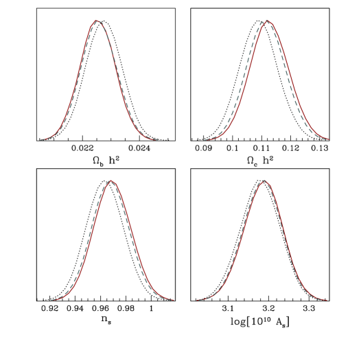
Figure 8: Dependence of parameter estimates on the shape of the source correction. Curves refer to default WMAP 5yr estimates (black/dotted lines), or our prediction when masking sources as described in the text (red/solid) or simply masking sources with $S_{41}>1$ Jy (green/dashed).

7 Summary and conclusions

We discussed a new method aimed at evaluating the residual point source contribution to the WMAP5 power spectrum. We implemented a stochastic approach to extrapolate the flux of radio sources of the NRAO-VLA Sky Survey (NVSS) to WMAP frequencies. Using different point source catalogs with multifrequency information, we divided the $1.4-90$ GHz in a number of frequency steps. At each step an NVSS source is randomly paired to a reference source in the catalog covering the relevant frequency range, and extrapolated to the upper limit of that range using the spectral index of the reference source. The procedure is iterated 800 times, and the ensemble of simulations provides the probability distribution for the flux each NVSS at the desired frequencies.

We compared the statistical properties of the simulations with those of the sources of the WMAP5 catalog, with other surveys at 33 GHz and with predictions by previous authors at 94 GHz, finding an agreement down for fluxes $\gtrsim 0.1$ Jy in Ka band, while we underestimate the number of sources below $\sim 0.1$ Jy. The WMAP catalog is not complete below $S\sim 1$ Jy, so point sources with $S\sim 0.1$ Jy account for only a small fraction of the total power due to unresolved sources. At higher frequencies predictions are in general agreement with previous works.

An advantage of the method is that it maintains the information about the sources position. In order to test this, we considered the sets of point-source-only (i.e. no CMB nor noise) maps obtained from NVSS simulations at 41 and 94 GHz, and correlated them with both the Q and W band WMAP5 sky maps and with mock CMB skies in which the point source population follows the same distribution as our model. We found that although the overall level of correlation is low, W band correlations with actual data are in good agreement with correlations with the mock data. In Q band, instead, the degree of correlation between simulations and actual maps is significantly lower than what expected from the mock data. In this band foregrounds contamination is significantly higher than at higher frequency and may contribute to decreasing the level of correlation between simulations and real maps.

We used the simulated maps to estimate the unresolved source correction to WMAP5 measured spectra. As a general result, we find that unresolved sources in our simulations have a steeper frequency behaviour than the contribution estimated by the WMAP team. This is due to the fact that observation of sources in the 20–90 GHz range with $S\lesssim 1$ Jy typically show steeper spectral indexes than the best fit spectral index from the WMAP5 catalog. The observed scaling in the simulations corresponds to an effective spectral index $\alpha=-0.20\sim-0.25$, compared to WMAP5 $\alpha=0\sim-0.09$. Thus, the unresolved point sources contribution derived by the simulation either agrees with the WMAP5 estimates in Q band but is lower by up to $\sim 30-40\%$ at 94 GH, depending on the way we mask bright sources. The corresponding shift in estimates for parameter like $n_{S}$ and $\omega_{c}$ can reach up to $\sim 0.3-0.4\sigma$.

Given a sufficient number of simulations, the approach followed in this work allows in principle to estimate the probability distribution for the flux at an arbitrary frequency of each source from a template low frequency survey. In turn this would allow to naturally account for the added uncertainty due to undetected sources during the map-making stage, as is done for galactic foregrounds with Gibbs sampling methods. This would require that Gibbs samplers can be made to efficiently work at multipoles $\ell\simeq 2000-3000$, where point sources will be relevant for Planck and other possibly upcoming high-resolution experiments. Even if this were not possible, having an estimate of unresolved source contributions in each pixel would be helpful in defining a sky mask, e.g. by flagging all pixel in which the source contribution is expected to exceed a given threshold even if there is no actual detection of a point source in that region of the map.

References

- Babich & Pierpaoli (2008) Babich, D., & Pierpaoli, E. 2008, Phys. Rev. D, 77, 123011
- Becker et al. (2003) Becker, R. H., Helfand, D. J., White, R. L., Gregg, M. D., & Laurent-Muehleisen, S. A. 2003, VizieR Online Data Catalog, 8071, 0
- Best et al. (2005) Best, P. N., Kauffmann, G., Heckman, T. M., & Ivezić, Ž. 2005, MNRAS, 362, 9
- Bock et al. (2009) Bock, J., et al. 2009, arXiv:0906.1188
- Colombo et al. (2009) Colombo, L. P. L., Pierpaoli, E., & Pritchard, J. R. 2009, MNRAS, 398, 1621
- Condon et al. (1998) Condon, J. J., Cotton, W. D., Greisen, E. W., Yin, Q. F., Perley, R. A., Taylor, G. B., & Broderick, J. J. 1998, AJ, 115, 1693
- de Zotti et al. (2005) de Zotti, G., Ricci, R., Mesa, D., Silva, L., Mazzotta, P., Toffolatti, L., & González-Nuevo, J. 2005, A&A, 431, 893
- de Zotti et al. (2009) de Zotti, G., Massardi, M., Negrello, M., & Wall, J. 2009, The Astronomy and Astrophysics Review, 15
- Dunkley et al. (2009) Dunkley, J., et al. 2009, ApJS, 180, 306
- Fendt & Wandelt (2007) Fendt, W. A., & Wandelt, B. D. 2007, ApJ, 654, 2
- Franceschini et al. (1989) Franceschini, A., Toffolatti, L., Danese, L., & de Zotti, G. 1989, ApJ, 344, 35
- Friedman et al. (2009) Friedman, R. B., et al. 2009, ApJ, 700, L187
- Gold et al. (2009) Gold, B., et al. 2009, ApJS, 180, 265
- González-Nuevo et al. (2008) González-Nuevo, J., Massardi, M., Argüeso, F., Herranz, D., Toffolatti, L., Sanz, J. L., López-Caniego, M., & de Zotti, G. 2008, MNRAS, 384, 711
- Górski et al. (2005) Górski, K. M., Hivon, E., Banday, A. J., Wandelt, B. D., Hansen, F. K., Reinecke, M., & Bartelmann, M. 2005, ApJ, 622, 759
- Gregory et al. (1996) Gregory, P. C., Scott, W. K., Douglas, K., & Condon, J. J. 1996, ApJS, 103, 427
- Hill et al. (2009) Hill, R. S., et al. 2009, ApJS, 180, 246
- Hinshaw et al. (2003) Hinshaw, G., et al. 2003, ApJS, 148, 135
- Hivon et al. (2002) Hivon, E., Górski, K. M., Netterfield, C. B., Crill, B. P., Prunet, S., & Hansen, F. 2002, ApJ, 567, 2
- Huffenberger et al. (2006) Huffenberger, K. M., Eriksen, H. K., & Hansen, F. K. 2006, ApJ, 651, L81
- Huffenberger et al. (2008) Huffenberger, K. M., Eriksen, H. K., Hansen, F. K., Banday, A. J., & Górski, K. M. 2008, ApJ, 688, 1
- Kamionkowski et al. (1997) Kamionkowski, M., Kosowsky, A., & Stebbins, A. 1997, Physical Review Letters, 78, 2058
- Kimball & Ivezić (2008) Kimball, A. E., & Ivezić, Ž. 2008, AJ, 136, 684
- Komatsu et al. (2009) Komatsu, E., et al. 2009, ApJS, 180, 330
- Lewis & Bridle (2002) Lewis, A., & Bridle, S. 2002, Phys. Rev. D, 66, 103511
- Limon et al. (2009) Limon, M et al. 2009, http://lambda.gsfc.nasa.gov/data/map/doc/MAP_supplement.pdf
- Mason et al. (2009) Mason, B. S., Weintraub, L. C., Sievers, J. L., Bond, J. R., Myers, S. T., Pearson, T. J., Readhead, A. C. S., & Shepherd, M. C. 2009, arXiv:0901.4330
- Nolta et al. (2009) Nolta, M. R., et al. 2009, ApJS, 180, 296
- Pierpaoli (2003) Pierpaoli, E. 2003, ApJ, 589, 58
- Pierpaoli & Perna (2004) Pierpaoli, E., & Perna, R. 2004, MNRAS, 354, 1005
- The Planck Collaboration (2006) The Planck Collaboration 2006, arXiv:astro-ph/0604069
- Readhead et al. (2004) Readhead, A. C. S., et al. 2004, ApJ, 609, 498
- Sadler et al. (2006) Sadler, E. M., et al. 2006, MNRAS, 371, 898
- Sadler et al. (2008) Sadler, E. M., Ricci, R., Ekers, R. D., Sault, R. J., Jackson, C. A., & de Zotti, G. 2008, MNRAS, 385, 1656
- Sawangwit & Shanks (2009) Sawangwit, U., & Shanks, T. 2009, arXiv:0912.0524
- Scott & White (1999) Scott, D., & White, M. 1999, A&A, 346, 1
- Serra & Cooray (2008) Serra, P., & Cooray, A. 2008, Phys. Rev. D, 77, 107305
- Spergel & Zaldarriaga (1997) Spergel, D. N., & Zaldarriaga, M. 1997, Physical Review Letters, 79, 2180
- Tegmark & Efstathiou (1996) Tegmark, M., & Efstathiou, G. 1996, MNRAS, 281, 1297
- Toffolatti et al. (1998) Toffolatti, L., Argueso Gomez, F., de Zotti, G., Mazzei, P., Franceschini, A., Danese, L., & Burigana, C. 1998, MNRAS, 297, 117
- Vielva et al. (2003) Vielva, P., Martínez-González, E., Gallegos, J. E., Toffolatti, L., & Sanz, J. L. 2003, MNRAS, 344, 89
- Vieira et al. (2009) Vieira, J. D., et al. 2009, arXiv:0912.2338
- Waldram et al. (2007) Waldram, E. M., Bolton, R. C., Pooley, G. G., & Riley, J. M. 2007, MNRAS, 379, 1442
- Waldram et al. (2009) Waldram, E. M., Pooley, G. G., Davies, M. L., Grainge, K. J. B., & Scott, P. F. 2009, arXiv:0908.0066
- Watson et al. (2003) Watson, R. A., et al. 2003, MNRAS, 341, 1057
- Wright et al. (2009) Wright, E. L., et al. 2009, ApJS, 180, 283