Effect of extreme data loss on long-range correlated and anti-correlated signals quantified by detrended fluctuation analysis

Abstract

Detrended fluctuation analysis (DFA) is an improved method of classical fluctuation analysis for nonstationary signals where embedded polynomial trends mask the intrinsic correlation properties of the fluctuations. To better identify the intrinsic correlation properties of real-world signals where a large amount of data is missing or removed due to artifacts, we investigate how extreme data loss affects the scaling behavior of long-range power-law correlated and anti-correlated signals. We introduce a new segmentation approach to generate surrogate signals by randomly removing data segments from stationary signals with different types of long-range correlations. The surrogate signals we generate are characterized by four parameters: (i) the DFA scaling exponent $\alpha$ of the original correlated signal $u(i)$, (ii) the percentage $p$ of the data removed from $u(i)$, (iii) the average length $\mu$ of the removed (or remaining) data segments, and (iv) the functional form $P(l)$ of the distribution of the length $l$ of the removed (or remaining) data segments. We find that the global scaling exponent of positively correlated signals remains practically unchanged even for extreme data loss of up to 90%. In contrast, the global scaling of anti-correlated signals changes to uncorrelated behavior even when a very small fraction of the data is lost. These observations are confirmed on two examples of real-world signals: human gait and commodity price fluctuations. We further systematically study the local scaling behavior of surrogate signals with missing data to reveal subtle deviations across scales. We find that for anti-correlated signals even 10% of data loss leads to significant monotonic deviations in the local scaling at large scales from the original anti-correlated towards uncorrelated behavior. In contrast, positively correlated signals show no observable changes in the local scaling for up to 65% of data loss, while for larger percentage of data loss, the local scaling shows overestimated regions (with higher local exponent) at small scales, followed by underestimated regions (with lower local exponent) at large scales. Finally, we investigate how the scaling is affected by the average length, probability distribution and percentage of the remaining data segments in comparison to the removed segments. We find that the average length $\mu_{r}$ of the remaining segments is the key parameter which determines the scales at which the local scaling exponent has a maximum deviation from its original value. Interestingly, the scales where the maximum deviation occurs follow a power-law relationship with $\mu_{r}$. Whereas the percentage of data loss determines the extent of the deviation. The results presented in this paper are useful to correctly interpret the scaling properties obtained from signals with extreme data loss.

I Introduction

In real-world signals data can be missing or unavailable to a very large extent, especially in archaeological, geological and physiological recordings which often once recorded in the past can not be generated again. Knowing the effects which data loss may have on the correlations and other dynamical properties of the output signals of a given system is instrumental in accurately quantifying and modeling the underlying mechanisms driving the dynamics of the system. Significant data loss can also be caused by failure of the data collection equipment, as well as by the removal of artifacts or noise-contaminated data segments. To correctly interpret results obtained from correlated signals with missing data, it is important to understand how the dynamical properties of such signals are affected by the degree of data loss. Here we systematically investigate how loss of data changes the scaling properties of various long-range power-law anti-correlated and positively correlated signals. Specifically, we develop a segmentation approach to generate surrogate signals by randomly removing data segments from stationary long-range power-law correlated signals, and we study how the correlation properties are affected by (i) the percentage of removed data, (ii) the average length of the removed (or remaining) data segments and (iii) the functional form of the probability distribution of the removed (remaining) segments. We utilize the detrended fluctuation analysis (DFA) to quantify the effect of extreme data loss on the scaling properties of long-range correlated signals.

Scaling (fractal) behavior was first encountered in a class of physical systems Stanley (1995); Shlesinger (1987); Liebovitch (1994) which for a given “critical” value of their parameters, exhibit complex organization among their individual components, leading to correlated interactions over a broad range of scales. This class of complex systems are typically characterized by (i) multi-component nonlinear feedback interactions, (ii) non-equilibrium output dynamics, and (iii) high susceptibility and responsiveness to perturbations. Scaling behavior has been found in a diverse group of systems — ranging from earthquakes, to traffic jams and economic crashes, to neuronal excitations as well as the dynamics of integrated physiologic systems under neural control — and has been associated with the underlying mechanisms of regulation of these systems Ivanov et al. (1998); Ashkenazy et al. (2002). The output signals of such systems exhibit continuous fluctuations over multiple time and/or space scales Bassingthwaighte et al. (1994); Malik and Camm (1995), where the amplitudes and temporal/spatial organization of the fluctuations are characterized by absence of dominant scale, i.e., scale-invariant behavior. Due to the nonlinear mechanisms controlling the underlying interactions, the output signals of these systems are also typically non-stationary, which masks the intrinsic correlations. Traditional methods such as power-spectrum and auto-correlation analysis Hurst (1951); Mandelbrot and Wallis (1969); Stratonovich (1981) are not suitable for nonstationary signals.

DFA is a robust method suitable for detecting long-range power-law correlations embedded in nonstationary signals Peng et al. (1994); Taqqu et al. (1995). It has been successfully applied to a variety of fields where scale-invariant behavior emerges, such as DNA Peng et al. (1994, 1992, 1993); Buldyrev et al. (1993); Ossadnik et al. (1994); Stanley et al. (1994); Mantegna et al. (1994); Havlin et al. (1995a); Peng et al. (1995a); Havlin et al. (1995b); Mantegna et al. (1996); Buldyrev et al. (1998); Stanley et al. (1999); Li et al. (2003); Hackenberg et al. (2005), cardiac dynamics Peng et al. (1995b); Ho et al. (1997); Barbi et al. (1998); Ivanov et al. (1999); Pikkujämsä et al. (1999); Ashkenazy et al. (1999); Mäkikallio et al. (1999); Absil et al. (1999); Toweill et al. (2000); Bunde et al. (2000); Laitio et al. (2000); Ashkenazy et al. (2000, 2001); Ivanov et al. (2001); Kantelhardt et al. (2002); Karasik et al. (2002); Ivanov et al. (2004a); Bartsch et al. (2005); Schmitt and Ivanov (2007); Schmitt et al. (2009), human locomotion Hausdorff et al. (1995); Ashkenazy et al. (2002); Bartsch et al. (2007); Ivanov et al. (2009), circadian rhythm Hu et al. (2004); Ivanov et al. (2007); Ivanov (2007); Hu et al. (2007), neural receptors in biological systems Bahar et al. (2001), seismology Varotsos et al. (2003, 2009), meteorology Ivanova and Ausloos (1999), climate temperature fluctuations Koscielny-Bunde et al. (1998a, b); Talkner and Weber (2000); Bunde et al. (2001); Monetti et al. (2003); Bunde et al. (2005), river flow and discharge Montanari et al. (2000); Matsoukas et al. (2000), and economics Liu et al. (1997); Vandewalle and Ausloos (1997, 1998); Liu et al. (1999); Janosi et al. (1999); Ausloos et al. (1999); Roberto et al. (1999); Vandewalle et al. (1999); Grau-Carles (2000); Ausloos (2000); Ausloos and Ivanova (2000); Ausloos and Ivanova (2001a, b); Ivanov et al. (2004b). The DFA method may also help identify different states of the same system exhibiting different scaling behavior — e.g., the DFA scaling exponent $\alpha$ for heart-beat intervals is significantly different for healthy and sick individuals Peng et al. (1995b); Ashkenazy et al. (1999); Schmitt and Ivanov (2007) as well as for wake and sleep states Ivanov et al. (1999); Bunde et al. (2000); Kantelhardt et al. (2002); Ivanov (2007); Schmitt et al. (2009).

Elucidating the intrinsic mechanisms of a given system requires an accurate analysis and proper interpretation of the dynamical (scaling) properties of its output signals. It is often the case that the scaling exponent quantifying the temporal (spatial) organization of the systems’ dynamics across scales is not always the same, but depends on the scale of observation, leading to distinct crossovers — i.e., the value of the scaling exponent may be different for smaller compared to larger scales. Such behavior has been observed for diverse systems, for example: (i) the spontaneous motion of microbeads bound to the cytoskeleton of living cells as quantified by the mean-square displacement does not exhibit a Brownian motion but instead undergoes a transition from subdiffusive to superdiffusive behavior with time Metzner et al. (2007); (ii) cardiac dynamics of healthy subjects during sleep are characterized by fluctuations in the heartbeat intervals exhibiting a crossover from a higher scaling exponent (stronger correlations) at small time scales (from seconds up to a minute) to a lower scaling exponent (weaker correlations) at large time scales (from minutes to hours), associated with changes in neural autonomic control during sleep Ivanov et al. (1999); Kantelhardt et al. (2003); and (iii) stock market dynamics where both absolute price returns and intertrade times exhibit a crossover from a lower scaling exponent at small time scales (up to a trading day) to much higher exponent at large time scales (from a trading day to many months), a behavior consistent for all companies on the market Liu et al. (1999); Ivanov et al. (2004b). However, crossovers may also be a result of various types of nonstationarities and artifacts present in the output signals, which, if not carefully investigated, may lead to incorrect interpretation and modeling of the underlying mechanisms regulating the dynamics of a given system Schmitt and Ivanov (2007).

In previous studies, we have systematically investigated the effects of various types of nonstationarities, data pre-processing filters and data artifacts on the scaling behavior of long-range power-law correlated signals as measured by the DFA method Hu et al. (2001); Chen et al. (2002, 2005). In particular, we studied a type of nonstationarity which is caused by the presence of discontinuities (gaps) in the signal, i.e., how randomly removing data segments of fixed length affects the scaling properties of long-range power-law correlated signals Chen et al. (2002). Such discontinuities may arise from the nature of the recordings — e.g., stock exchange data are not recorded during the nights, weekends and holidays Liu et al. (1997); Vandewalle and Ausloos (1997, 1998); Liu et al. (1999); Janosi et al. (1999); Ausloos et al. (1999); Roberto et al. (1999); Vandewalle et al. (1999). In these situations, discontinuities correspond to segments of fixed size.

Alternatively, discontinuities may be caused by the fact that (i) part of the data is lost due to various reasons, and/or (ii) some noisy and unreliable portions of continuous recordings (e.g., measurement artifacts) are discarded prior to analysis Peng et al. (1995b); Ho et al. (1997); Barbi et al. (1998); Ivanov et al. (1999); Pikkujämsä et al. (1999); Ashkenazy et al. (1999); Mäkikallio et al. (1999); Absil et al. (1999); Toweill et al. (2000); Bunde et al. (2000); Laitio et al. (2000); Ashkenazy et al. (2000, 2001); Ivanov et al. (2001); Schmitt et al. (2009). In these cases, the lengths of the lost or removed data segments are random, and may follow a certain type of distribution which can often be related to the process responsible for the removal or loss of data — e.g., a data acquisition device which fails randomly with a given probability $p$ will result in a geometric distribution $P(l)=(1-p)^{l}p$ with mean $\mu=1/p$, where $l$ is the length of the data lost segments. Thus, investigating the effect of data loss is essential to determine the true correlation properties of the signal output of a given system.

To address this question, we propose a new segmentation algorithm to generate surrogate signals by randomly removing data segments from long-range power-law correlated signals with a-priori known scaling properties, and we investigate the effects of the percentage of the removed data, different average lengths and different distributions of removed data segments. We compare the scaling behavior of the original signals with the scaling of the surrogate signals by systematically studying changes in the DFA scaling exponent. We utilize local scaling exponents to reveal subtle deviations and to characterize changes in the scaling behavior at different scales in signals with segment removed. We note, that in our investigation we consider the effect of data loss on signals where the scaling behavior remains constant for the duration of the observations. Signals comprised of segments characterized by different scaling exponents have been considered elsewhere Chen et al. (2002).

This paper is structured as follows: in Sec. II.1, we briefly describe the DFA method. In Sec. II.2 we describe how to generate stationary long-range power-law correlated signals. In Sec. II.3 we introduce an algorithm for randomly removing data segments from these signals to test the effects of data loss on the scaling behavior. In Sec. III.1, we study the effect of data loss on the global scaling of positively correlated and anti-correlated artifically generated signals with different length, and we show examples on two different sets of empirical data. In Sec. III.2 we compare the local scaling properties of correlated signals before and after data removal by considering the effect of several parameters of the removed segments. In Sec. III.3 we consider the inverse situation — instead of focusing on the properties of the removed segments we investigate how the correlations/scaling of the signal depend on the properties of the remaining data segments. We summarize and discuss our findings in Sec. IV.

II Methods

II.1 Detrended fluctuation analysis (DFA)

The DFA is a random walk based method Peng et al. (1994). It is an improvement of the classical fluctuation analysis (FA) for nonstationary signals where embedded polynomial trends mask the intrinsic correlation properties in the fluctuations Peng et al. (1994). The performance of DFA for signals with different types of nonstationarities and artifacts has been extensively studied and compared to other methods of correlation analysis Taqqu et al. (1995); Hu et al. (2001); Chen et al. (2002, 2005); Xu et al. (2005); Alvarez-Ramirez et al. (2005); Nagarajan (2006); Bashan et al. (2008). The DFA methods involves the following steps Peng et al. (1994):

(i) A given signal $u(i)$ ($i=1,..,N$, where $N$ is the length of the signal) is integrated to obtain the random walk profile $y(k)\equiv\sum_{i=1}^{k}[u(i)-\langle u\rangle]$, where $\langle u\rangle$ is the mean of $u(i)$.

(ii) The integrated signal $y(k)$ is divided into boxes of equal length $n$.

(iii) In each box of length $n$ we fit $y(k)$ using a polynomial function of order $\ell$ which represents the trend in that box. The $y$ coordinate of the fit curve in each box is denoted by $y_{n}(k)$. When a polynomial fit of order $\ell$ is used, we denote the algorithm as DFA-$\ell$. Note that, due to the integration procedure in step (i), DFA-$\ell$ removes polynomial trends of order $\ell-1$ in the original signal $u(i)$.

(iv) The integrated profile $y(k)$ is detrended by subtracting the local trend $y_{n}(k)$ in each box of length $n$:

$$Y(k)\equiv~{}y(k)-y_{n}(k).$$ (1)

(v) For a given box length $n$, the root-mean-square (rms) fluctuation function for this integrated and detrended signal is calculated:

$$F(n)\equiv\sqrt{{1\over{N}}\sum_{k=1}^{N}[Y(k)]^{2}}.$$ (2)

(vi) The above computation is repeated for a broad range of box lengths $n$ (where $n$ represents a specific space or time scale) to provide a relationship between $F(n)$ and $n$.

A power-law relation between the root-mean-square fluctuation function $F(n)$ and the box size $n$, i.e., $F(n)\sim n^{\alpha}$, indicates the presence of scaling-invariant behavior embedded in the fluctuations of the signal $u(i)$. The fluctuations can be characterized by a scaling exponent $\alpha$, a self-similarity parameter which represents the long-range power-law correlation properties of the signal. If $\alpha=0.5$, there is no correlation and the signal is uncorrelated (white noise); if $\alpha<0.5$, the signal is anti-correlated; if $\alpha>0.5$, the signal is positively correlated; and $\alpha=1.5$ indicates Brownian motion (integrated white noise). For stationary signals with long-range power-law correlations, the value of the scaling exponent $\alpha$ is related to the exponent $\beta$ characterizing the power spectrum $S(f)=f^{-\beta}$ of the signal, where $\beta=2\alpha-1$ Peng et al. (1993). Thus, the special case of $1/f$ noise, where $\beta=1$, observed in various physiological and biological system dynamics, corresponding to $\alpha=1$. Since the power spectrum of stationary signals is the Fourier transform of the auto-correlation function, for signals with scale-invariant long-range positive correlation and $\alpha<1$, one can find the following relationship between the auto-correlation exponent $\gamma$ and the power spectrum exponent $\beta$ for signals with scale-invariant long-range correlations: $\gamma=1-\beta=2-2\alpha$, where $\gamma$ is defined by the auto-correlation function $C(\tau)=\tau^{-\gamma}$, and should satisfy $0<\gamma<1$ Kantelhardt et al. (2001).

We note that for anti-correlated signals, the scaling exponent $\alpha$ obtained from the DFA method overestimates the true correlations at small scales $n$ Hu et al. (2001). To avoid this problem, one needs first to integrate the original anti-correlated signal and then apply the DFA method. The correct scaling exponent can thus be obtained from the relation between $n$ and $F(n)/n$ [instead of $F(n)$] (see Fig. 4a). This procedure is applied for all cases of anti-correlated signals in this study. In our analysis in the following sections we apply DFA-2. The choice of DFA-2 is dictated by the fact that this order of DFA-$l$ can accurately quantify the scaling behavior of signals with exponents in the range $0<\alpha<3$ Xu et al. (2005), which covers practically all signals generated by real world systems. Moreover, earlier investigations have demonstrated that DFA-2 is sufficient to accurately quantify a broad range of nonstationary signals generated by different physiologic dynamics — e.g., for heartbeat and gait dynamics the exponent $\alpha$ obtained from higher order DFA-$l$ is not significantly different compared to $\alpha$ obtained from DFA-2 Ivanov et al. (2009). Further, deviations from scaling which appear at small scale become more pronounced in higher order DFA-$l$ Kantelhardt et al. (2001). In order to provide an accurate estimate of $F(n)$, the largest box size $n$ we use is $n=N/8$, where $N$ is the signal length.

II.2 Procedure to generate stationary signals with long-range power-law correlations

We use a modified Fourier filtering technique Makse et al. (1996) to generate stationary long-range power-law correlated signals $u(i)$ ($i=1,2,...,N$) with mean $\langle u(i)\rangle=0$ and standard deviation $\sigma=1$. The correlations of $u(i)$ are characterized by a Fourier power spectrum of a power-law form $S(f)\sim f^{-\beta}$, where $f$ is the frequency. By manipulating the Fourier spectrum of random Gaussian-distributed sequences, we generate signal $u(i)$ with desired power-law correlations. This method consists of the following steps:

(i) First, we generate a Gaussian-distributed sequence $\eta(i)$ with mean $\langle\eta(i)\rangle=0$ and standard deviation $\sigma_{\eta}=1$, and we calculate its Fourier transformation $\hat{\eta}(f)$.

(ii) Next, we generate $\hat{u}(f)$ using the following transformation:

$$\hat{u}(f)=\hat{\eta}(f)\cdot f^{-\beta/2},$$ (3)

where $\hat{u}(f)$ is the Fourier transform of the desired correlated signal $u(i)$ characterized by a Fourier power spectrum of the form

$$S(f)=|\hat{u}(f)|^{2}\sim f^{-\beta},$$ (4)

(iii) We calculate the inverse Fourier transform of $\hat{u}(f)$ to obtain $u(i)$. The generated stationary signal $u(i)$ is then normalized to zero mean and unit standard deviation.

II.3 Algorithm to generate surrogate signals with randomly removed segments

We introduce a new segmentation approach to generate surrogate nonstationary signals $\tilde{u}(i)$ by randomly removing data segments from a stationary correlated signal $u(i)$ and stitching together the remaining parts of $u(i)$. Such “cutting” procedure is often used in the pre-processing of data prior to analysis in order to eliminate, for example, segments of data artifacts. The proposed segmentation approach allows the simulation of empirical data series where data segments are lost or removed. The surrogate signals $\tilde{u}(i)$ are characterized by four parameters: (i) the DFA scaling exponent $\alpha$ of the original signal $u(i)$, (ii) the percentage $p$ of the data removed, (iii) the average length $\mu$ of the removed data segments as well as (iv) the functional form $P(l)$ of the distribution of the length $l$ of the removed data segments.

To generate a surrogate signal $\tilde{u}(i)$ from the original signal $u(i)$, we first construct a binary sequence $g(i)$ with the same length $N$ as $u(i)$. In our algorithm the positions $i$ where $g(i)=0$ will correspond to the positions at which data points in $u(i)$ are removed, while the positions where $g(i)=1$ will correspond to the positions in $u(i)$ where data points are preserved (Fig. 1).

Figure 1: Illustration of generating a surrogate signal $\tilde{u}(i)$ by removing data points from the original signal $u(i)$ according to a binary series $g(i)$. The positions $i$ where $g(i)=0$ (or 1) correspond to the positions at which data points in $u(i)$ are removed (or preserved) to obtain $\tilde{u}(i)$.

We developed the following method to construct the binary series $g(i)$:

(i) We generate the lengths $l_{j}$ ($j=1,2,...,M$) of the segments that will be removed from the original signal $u(i)$ by randomly drawing integer numbers from a given probability distribution $P(l)$ with mean value $\mu$. Each integer number drawn from $P(l)$ represents the length of a segment removed from $u(i)$. The process continues until the summation of the lengths of all removed segments becomes equal or exceeds a predetermined amount $pN$ of data to be removed, i.e.,

$$\sum_{j=1}^{M}l_{j}~{}\geq~{}pN,$$ (5)

where $M$ is the minimal number to fulfill Eq. 5. Eventually, we will cut the size of the last segment to obtain the exact fraction $pN$ of the lost data.

(ii) We append a “1” to each element in the series $\{l_{j}\}$ which will serve as a separator between two adjacent segments (see step (iv)), and results in a new series $\{[l_{j},1]\}$. Note that now the summation over the series yields $pN+M$.

(iii) We append $N-(pN+M)$ “1” elements to the end of the series $\{[l_{j},1]\}$ to obtain an extended series where the sum of all elements is $N$, equal to the length of the original series $u(i)$. This extended series is then shuffled leading to a set of $M$ elements $[l_{j},1]$ randomly scattered in a “sea” of $N-(pN+M)$ “1” elements (see Eq. 6).

(iv) Next, we replace the numbers $l_{j}$ in Eq. 6 with $l_{j}$ elements of zeros, to obtain a binary series $g(i)$ as shown in Eq. 7.

$$\{\ldots,1, \ \ \ \ [l_{j},1], 1,\ldots,1, \ \ [l_{j+1},1], [l_{j+2},1],\ \ 1,\ldots\}$$ (6)

$$\{\ldots,1, \overbrace{0,\ldots,0,1}, 1,\ldots,1, \overbrace{0,\ldots,0,1}, \overbrace{0,\ldots,0,1}, 1,\ldots\}$$ (7)

Note that, in step (iii) of our algorithm, the shuffling of the extended series may lead to two or more $[l_{j},1]$ elements, which represent removed data segments, to become direct neighbors (Eq. 6). Adding “1” to each element $\{l_{j}\}$ in step (ii) thus ensures that adjacent $[l_{j},1]$ elements in the shuffled extended series in Eq. 6 would not allow two or more separate removed segments to be merged leading to the formation of removed segments with longer average length $\mu$ and different form of their probability distribution compared to the original choice in step (i) of the algorithm.

Finally, the surrogate signal $\tilde{u}(i)$ is obtained by simultaneously scanning the original signal $u(i)$ and the binary series $g(i)$ from Eq. 7, removing the $i$-th element in $u(i)$ if $g(i)\equiv 0$ and concatenating the segments of the remaining data (Fig. 1).

In this study, we consider four different functional forms of the probability distribution $P(l)$ of segment lengths $l$, i.e., exponential, Gaussian, $\delta$- and power-law distributions, and we use the average length $\mu$ of the removed data segments as a common parameter to compare the effect of removed data segments with different distributions. For the exponential and $\delta$-distribution, the average length $\mu$ is sufficient to determine their probability distribution functions. The Gaussian and power-law distributions require additional parameters to be clearly defined, and thus, we need to introduce boundary conditions, so that these parameters can be related to the average length $\mu$.

The functional form of the Gaussian distribution is

$$P(l)=\frac{1}{\sqrt{2\pi\sigma^{2}}}exp\left[-\frac{(l-\mu)^{2}}{2\sigma^{2}}\right],$$ (8)

where $\mu$ is the average and $\sigma$ is the standard deviation of the segment lengths $l$. Since with a fixed small $\sigma$, the Gaussian distribution is not much different from a $\delta$-distribution, and with a fixed large $\sigma$, the Gaussian distribution resembles an exponential distribution, we relate $\sigma$ with $\mu$ in such a way, as a boundary condition, that the smallest segment ($l=1$) can only be obtained (statistically) once in each realization, i.e., $P(l=1)~{}\equiv~{}1/pN$, where $N$ is the length of the original signal, and $p$ is the percentage of data loss.

The functional form of a power-law distribution is given by

$$P(l)=al^{k},l\in[1,l_{max}],$$ (9)

with $\int_{1}^{l_{max}}P(l)dl=1$ and the average length $\mu=\int_{1}^{l_{max}}lP(l)dl$. Similar to the Gaussian distribution, we set the probability of the largest segment to $P(l=l_{max})~{}\equiv~{}1/pN$. With these three boundary conditions, we can relate the three parameters $a$, $k$ and $l_{max}$ in Eq. 9 with the average length $\mu$.

In Fig. 2, we show examples of Gaussian and power-law distributions with different average lengths $\mu$ based on the criteria described above. Fig. 3 shows examples of our procedure of data removal. The lengths of the removed segments were chosen to be exponentially distributed with different average length.

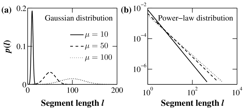
Figure 2: Examples of theoretical probability density for (a) Gaussian distribution and (b) power-law distribution used in our simulations of different situations of data loss. The parameters for the functional form of distributions are determined by the average length $\mu$ we chose for each simulation and by specific boundary conditions, i.e., for the Gaussian distribution, we set the probability of the smallest segment length $P(l=1)=1/pN$, and for the power-law distribution we set the probability of the largest segment length $P(l=l_{max})=1/pN$ (see text for details).

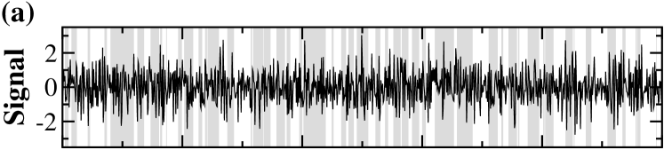
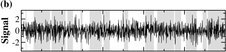
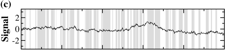
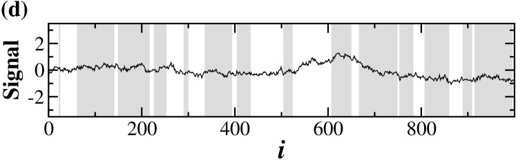
Figure 3: Illustration of data removal from stationary correlated signals. Removed data segments (shaded regions) are randomly positioned within the original signal, and their lengths $l$ are drawn from an exponential distribution $P(l)~{}=~{}\frac{1}{\mu}\exp(-l/\mu)$ with average value $\mu$. An average length $\mu=10$ is chosen for (a) the anti-correlated signal (DFA scaling exponent $\alpha=0.3$) and (b) the positively correlated signal ($\alpha=1.3$). Larger segments with $\mu=50$ are removed from (b) anti-correlated signal ($\alpha=0.3$) and (d) positively correlated signal ($\alpha=1.3$).

III Results

III.1 Effect of data loss on global scaling

Previously, we have studied the effect of data loss on the scaling behavior of long-range correlated signals by removing data segments with fixed length Chen et al. (2002). We have found that data loss in anti-correlated signals substantially changes the scaling behavior even when only 1% of data are removed. In contrast, the scaling behavior of (positively) correlated signals is practically not affected even when up to 50% of the data are removed. Data loss generally causes a crossover in the scaling behavior of anti-correlated signals. At the scales larger than the crossover the anti-correlated scaling behavior is completely destroyed and resembles uncorrelated behavior. This crossover is shifted to smaller scales with increasing percentage of removed data or decreasing length of the removed segments, indicating a stronger effect on the scaling behavior.

In most cases, the length of data loss segments is not fixed but random, and follows a certain distribution. How does the distribution of data loss segments influence the scaling behavior of correlated signals? In some cases, especially when archaeological data are studied, the percentage of data loss can be extremely large (and can reach up to 95% ! Temin (2002)). Would the extreme data loss affect also positively correlated signals? To address these questions, in this section we study the effect of data loss caused by random removal of data segments that follow a certain distribution.

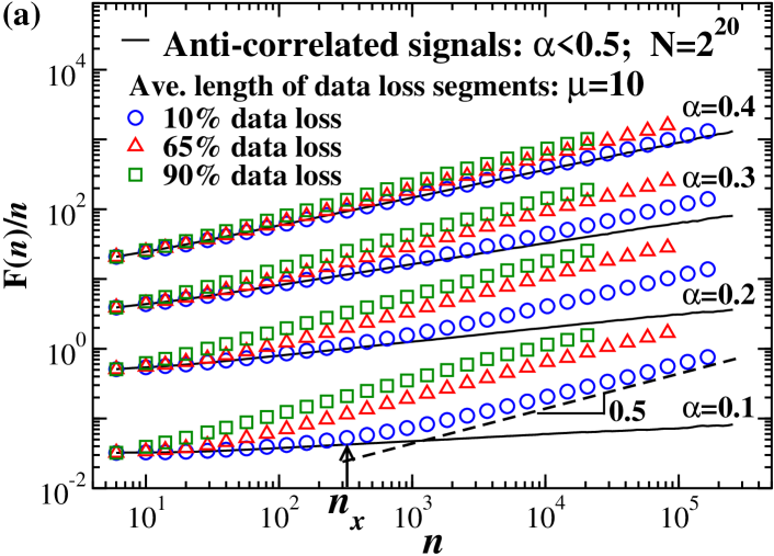
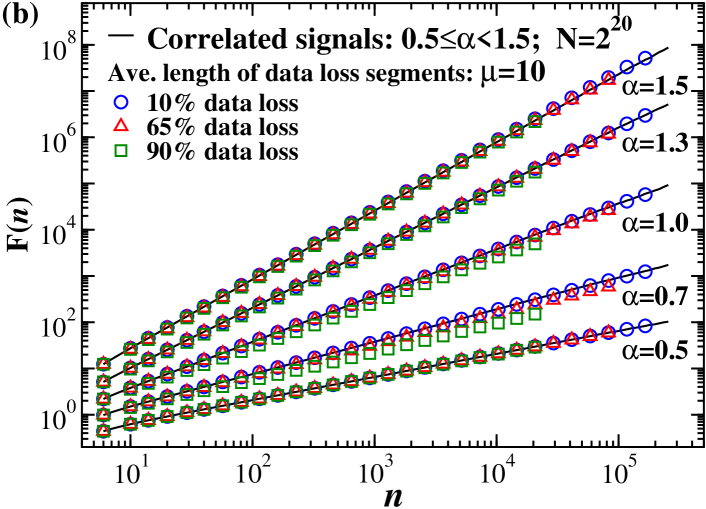
Figure 4: (Color online) Effect of data loss on the scaling behavior of long-range correlated signals with length $N=2^{20}$ (before data removal), zero mean and unity standard deviation. The lengths of the removed segments are drawn from an exponential distribution with mean $\mu=10$. (a) Scaling behavior of anti-correlated signals (scaling exponent $\alpha<0.5$) with a data loss of 10% (blue circles), 65% (red triangles) and 90% (green squares). Note that, to obtain an accurate estimation of the DFA scaling exponent $\alpha$ for anti-correlated signals, we first integrate the signals and then we apply the DFA method. Thus, to obtain the correct scaling exponent for anti-correlated signals we divide $F(n)$ by $n$ to account for the integration of the signals and next we plot $F(n)/n$ vs. the scale $n$ (see also Sec. II.1 and Fig. 15 in Hu et al. (2001)). (b) Scaling behavior of positively correlated signals (scaling exponent $\alpha>0.5$) with 10%, 65% and 90% data loss. The scaling behavior of strongly anti-correlated data is dramatically changed even when only 10% of the data are removed. A crossover at scale $n_{x}$ indicates a transition (arrow), due to loss of data in the signals, from the original anti-correlated behavior with $\alpha=0.1$ to an uncorrelated behavior with $\alpha=0.5$. In contrast, for positively correlated signals, i.e. $0.5<\alpha<1.5$ only an extreme data loss of 90% leads to small deviations from the original scaling behavior. This effect becomes weaker for increasing values of $\alpha$ . As expected, for $\alpha=0.5$ (white noise) and $\alpha=1.5$ (Brownian noise) data removal does not affect the scaling behavior.

First, we consider the case in which the lengths of data loss segments are exponentially distributed. Following the approach introduced in Sec. II.3, we first generate stationary correlated signals $u(i)$ with length $N=2^{20}$ and with scaling exponents $\alpha$ ranging from 0.1 to 1.5, and then randomly remove exponentially distributed data segments from the original signal $u(i)$ to obtain surrogate signals $\tilde{u}(i)$. As illustrated in Fig. 4, the rms fluctuation function $F(n)$ shows similar changes in the scaling behavior as observed in Chen et al. (2002) where segments with a fixed length were removed from the original signal. (i) The scaling behavior of surrogate signals strongly depends on the scaling exponent $\alpha$ of the original signals. (ii) The anti-correlated signals substantially change their scaling behavior even if only 10% of the data are removed (Fig. 4(a)). A crossover from anti-correlated to uncorrelated ($\alpha=0.5$) behavior appears at scale $n_{x}$ due to data loss, i.e., at the scales larger than $n_{x}$, the anti-correlations in the original signals are completely destroyed. The crossover scale $n_{x}$ is shifted to smaller scales with increasing percentage of lost data. (iii) In contrast, positively correlated signals show practically no changes for up to 65% of data loss (Fig. 4(b)). Surprisingly, even with extreme data loss of up to 90% of the signal the scaling behavior is still practically preserved, exhibiting a slightly lower exponent $\alpha$ (waker correlations) — an effect which is less pronounced with increasing values of $\alpha$ (see Fig. 4(b)).

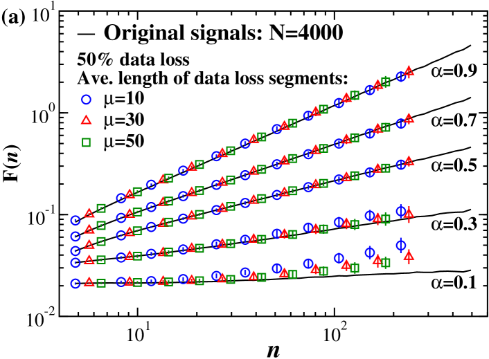
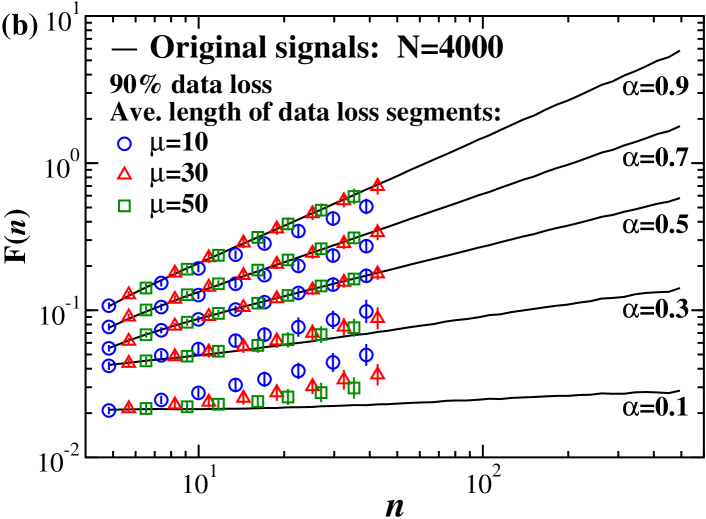
Figure 5: (Color online) Effect of data loss on the scaling behavior of short signals ($N=4000$ before data removal). (a) Removing up to 50% of the data (i.e., 2000 data points remain) does not have an observable effect on the scaling behavior of positively correlated signals and leads to small deviations from the original scaling behavior in anti-correlated signals. (b) Extreme data loss of 90% (i.e., only 400 data points remain) leads to more pronounced deviations from the original scaling behavior. In general, the deviations are smaller with larger average length $\mu$ of removed segments.

Next, we consider the case in which the length of the original signal is much shorter ($N=4000$), as illustrated in Fig. 5. We find that the scaling behavior of both anti-correlated and positively correlated signals with extreme data loss change in the same way as we observed in Fig. 4 (where $N=2^{20}$). In addition, we find (see Fig. 5) that when increasing the average length $\mu$ of the data loss segments, the scaling behavior of the surrogate signals deviates less from the original scaling behavior. Thus, removing the same percentage of the data using longer (and fewer) segments has a lesser impact on the scaling behavior of both positively correlated and anti-correlated signals compared to removing segments with smaller average length $\mu$.

To show how missing data segments affect correlations in real-world signals, we consider two examples of complex scale-invariant dynamics: (i) human gait as a representative of integrated physiologic systems under neural control with multiple-component feedback interactions (Fig. 6a), and (ii) commodity price fluctuations from England across several centuries reflecting complex economic and social interactions (Fig. 6b). In agreement with our tests on surrogate signals shown in Fig. 4 and Fig. 5, our analyses of real data confirm the observation that even extreme data loss of up to 90% does not significantly affect the global scaling behavior of positively correlated ($\alpha>0.5$) signals.

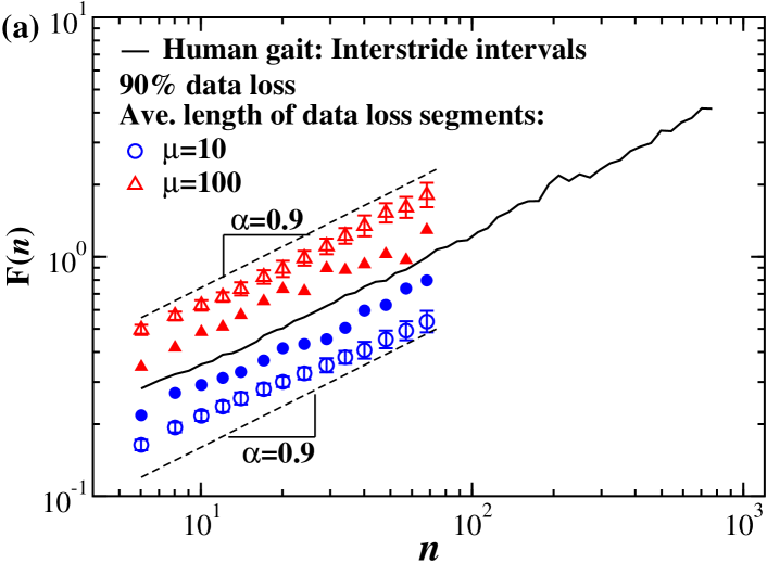
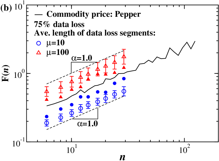
Figure 6: (Color online) Two examples of the effect of extreme data loss: (a) interstride intervals of human gait, and (b) annual prices of pepper in England in the period 1209–1914. Removing up to 90% of the gait intervals and up to 75% of the commodity data using segments of different average length $\mu$ does not significantly affect the global scaling behavior. Closed symbols represent a single realization and open symbols indicate the mean and standard deviations obtained from 100 realizations of randomly removing data segments. The lengths of the removed data segments are drawn from an exponential distribution.

III.2 Properties of removed data segments: Effect of data loss on local scaling

To reveal in greater detail the effect of data loss, we investigate the local scaling behavior of the $F(n)$ curves by fitting $F(n)$ locally in a window of size $w=3log2$. We determine the local scaling exponent $\alpha_{loc}$ at different scales $n$ by moving the window $w$ in small steps of size $\Delta=\frac{1}{4}log2$ starting at $n=4$.

In Fig. 7, we show $\alpha_{loc}$ for 10%, 65% and 90% of data loss, and the average length of the data loss segments is $\mu=10$ (cp. Fig. 4). The scaling behavior of anti-correlated signals shows systematic deviations from the original behavior: the stronger the anti-correlations, the faster is the decay of $\alpha_{loc}$ towards 0.5 (uncorrelated behavior). The deviations are stronger when more data were removed from the original signal. Note that when 90% of the data are removed, the correlation properties of originally anti-correlated signals are completely destroyed (Fig. 7(c)), because there are practically no consecutive data points of the original signals preserved in the surrogates when $\mu=10$ and $p=90\%$ (see Sec. III.3 and Eq. 10). When increasing the average length of the removed segments from $\mu=10$ to $\mu=100$ (Fig. 7), the scaling behavior of anti-correlated signals is less affected and $\alpha_{loc}=0.5$ is reached at larger scales.

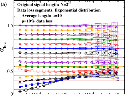
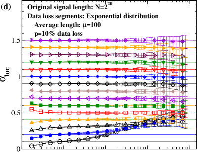
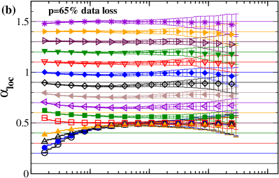
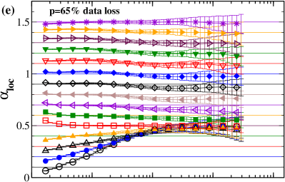
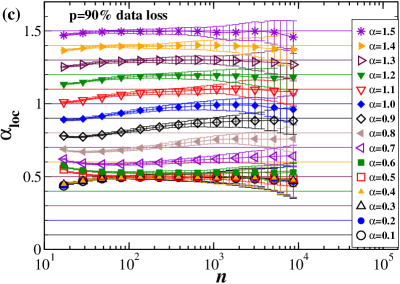
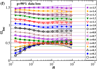
Figure 7: (Color online) Effect of data loss on the local scaling behavior (quantified by local scaling exponent $\alpha_{loc}$) of long-range power-law correlated signals. The symbols indicate average $\alpha_{loc}$ values obtained from 100 different realizations of surrogate signals with the same correlation exponent $\alpha$, and the error bars show the standard deviations. The more data are removed, the more the scaling exponent deviates from the original exponent. The data loss segments are exponentially distributed with average length $\mu=10$ ((a)-(c)) and $\mu=100$ ((d)-(f)). For anti-correlated signals, the removal of larger segments ($\mu=100$) has less effect on the scaling behavior. For positively correlated signals, the deviations vary across scales, showing both overestimated and underestimated regions.

For positively correlated signals ($0.5<\alpha<1.5$), the effect of data loss is more complex. The local scaling exponents show significant and systematic deviations from the original scaling behavior not observed in the rms fluctuation functions $F(n)$ in Fig. 4(b). The deviations from the original scaling behavior are more pronounced for a higher percentage of data loss and vary across scales. For small average length ($\mu=10$, Fig. 7a-c), the local scaling exponent is underestimated at small scales and gradually recovers to the original scaling behavior at larger scales. For a larger average length of removal data segments ($\mu=100$, Fig. 7d-f), we find overestimated regions at small scales and underestimated regions at large scales. The overestimation of the local scaling behavior is more pronounced for stronger positively correlated signals, while the underestimation is more pronounced for weaker positively correlated signals.

An interesting phenomenon seen in Fig. 7 is that for anti-correlated signals the scale at which $\alpha_{loc}$ reaches 0.5 (uncorrelated behavior) is shifted towards smaller scales with increasing percentage of data loss. Similarly, for positively correlated signals, the overestimated and underestimated regions are also shifted towards smaller scales, when a higher percentage of data is removed. This phenomenon occurs in both cases $\mu=10$ and $\mu=100$.

To understand precisely how the two parameters — the average length $\mu$ of the data loss segments and the percentage $p$ of data loss — influence changes in the local scaling behavior, in Fig. 8a-d we show how $\alpha_{loc}$ changes with the average length $\mu$ of the removed segments. For anti-correlated signals, the scale at which $\alpha_{loc}$ reaches 0.5 monotonically increases and shows a power-law relationship with $\mu$ (Fig. 8a). For positively correlated signals, as shown in Fig. 8b-d, the overestimated regions at small scales as well as the underestimated regions at large scales are shifted to higher scales with increasing $\mu$. This shift in the local scaling behavior also follows a power-law with average length $\mu$ (Fig. 8c, inset).

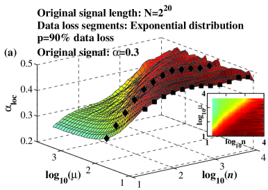
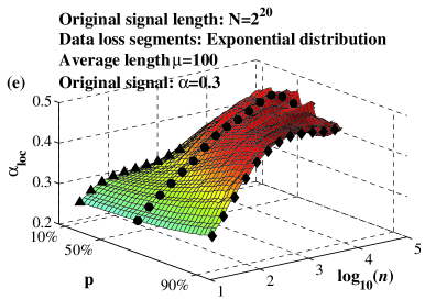
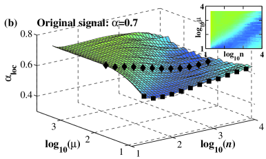
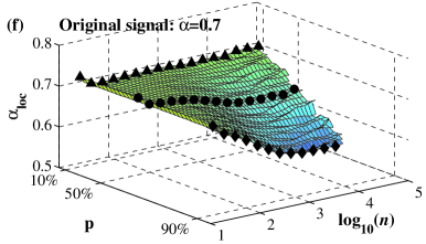
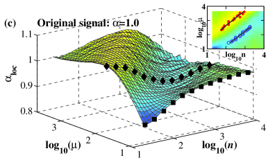
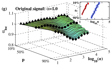
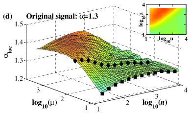
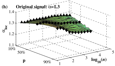
Figure 8: (Color online) Effect of the average length $\mu$ of data loss segments (a)-(d) and effect of the percentage $p$ of data loss (e)-(h) on the local scaling behavior in anti-correlated signals [(a), (e): $\alpha=0.3$] and positively correlated signals [(b), (f): $\alpha=0.7$; (c), (g): $\alpha=1.0$; (d), (h): $\alpha=1.3$]. For (a)-(d), $p=90\%$ of data are removed, and for (e)-(h), the average length of removed segments $\mu=100$. In all the cases, the removed segments are exponentially distributed, and the length of the original signals $N=2^{20}$. To clearly see the power-law relation between the average length $\mu$ of removed segments and the scale $n$ at which $\alpha_{loc}$ achieves the same value, the $\alpha_{loc}$ values are projected into the $\log_{10}\mu$–$\log_{10}n$ plane (see color-coded insets in figures (a)–(d)). The symbols in the inset figures in (c) and (g) indicate the positions where $\alpha_{loc}$ values reach a maximum (red closed circle) or a minimum (blue open circle), and depict the shift of the overestimated and underestimated regions to large scales with increasing $\mu$ and decreasing $p$. The local scaling curves highlighted by black symbols correspond to the curves shown in Fig. 7 (rectangle: $\mu=10$, $p=90\%$; diamond: $\mu=100$, $p=90\%$; circle: $\mu=100$, $p=65\%$; triangle: $\mu=100$; $p=10\%$).

In Fig. 8e-h, we show how the percentage $p$ of data loss influence changes in the local scaling behavior. For a fixed average length $\mu=100$, we find that the deviation from the original scaling behavior is more pronounced for higher values of $p$ in both anti-correlated and positively correlated signals, as also observed in Fig. 7. The scaling behavior of positively correlated signals also shows overestimated regions at small scales and underestimated regions at large scales (Fig. 8f-h), although not as clear as in Fig. 8b-d. Both regions are shifted to larger scales with decreasing percentage of data loss as illustrated in the inset in Fig. 8g.

To understand whether different functional forms of distributions of data loss segments have different effects on the scaling behavior, we repeated the same tests with three other kinds of distributions: a Gaussian distribution, a $\delta$-distribution (i.e., segments have fixed length) and a power-law distribution. We find that all three kinds of distributions show similar deviations from the original local scaling behavior as reported above for exponentially distributed data loss segments. However, for power-law distributed segments lengths, the estimated local scaling exponents are generally higher (lower) across scales for positively (anti-) correlated signals (Fig. 9). When increasing the average length $\mu$ of the removed data segments or increasing the percentage $p$ of data loss, the power-law distribution shows less variations than the other three kinds of distributions (Fig. 10 and Fig. 11).

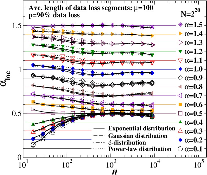
Figure 9: (Color online) Effect of different kinds of distributions of data loss segments on the local scaling behavior. The power-law distributed data loss segments lead to higher values of $\alpha_{loc}$ for positively correlated signals and lower values for anti-correlated signals compared to the other distributions. There is no difference between Gaussian and $\delta$-distributed segments which yield slightly lower $\alpha_{loc}$ values than exponentially distributed signals. For anti-correlated signals, exponentially, Gaussian and $\delta$-distributed segments lead to identical $\alpha_{loc}$ values whereas the power-law distribution yields slightly lower local scaling exponents.

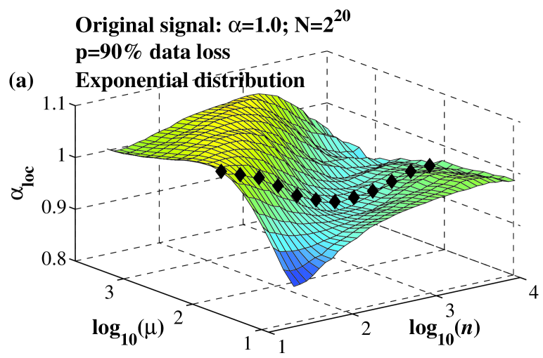
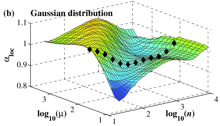
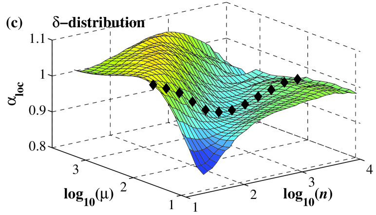
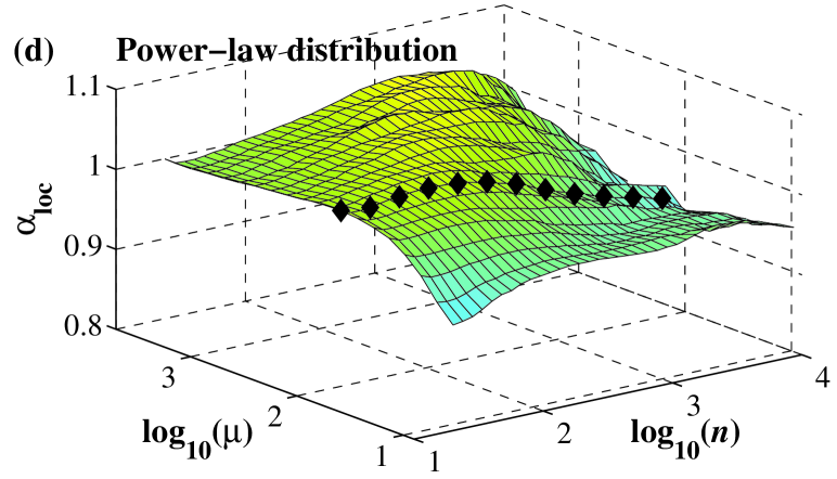
Figure 10: (Color online) Effect of the average length $\mu$ of data loss segments on the local scaling behavior in long-range correlated signal with $\alpha=1.0$. The length of the data loss segments are (a) exponentially distributed, (b) Gaussian distributed, (c) $\delta$-distributed and (d) power-law distributed. In all the cases, $p=90\%$ of data are removed, and the length of the original signals $N=2^{20}$. The behavior of how $\alpha_{loc}$ changes with $\mu$ is similar for exponential, Gaussian and $\delta$-distribution, while the power-law distribution shows less variations. The local scaling curves highlighted by black symbols correspond to the curves shown in Fig. 9.

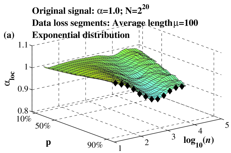
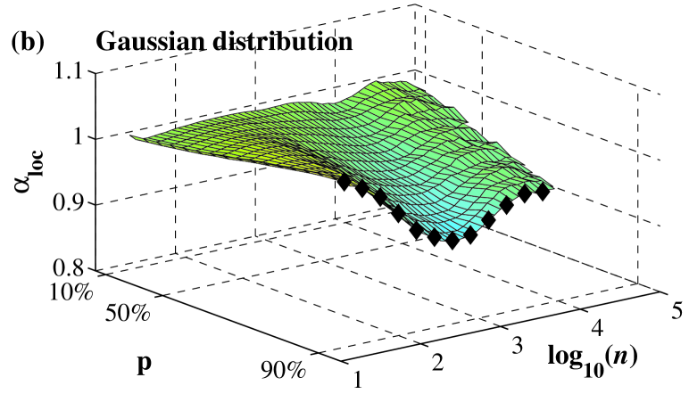
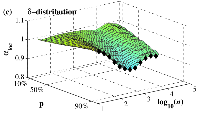
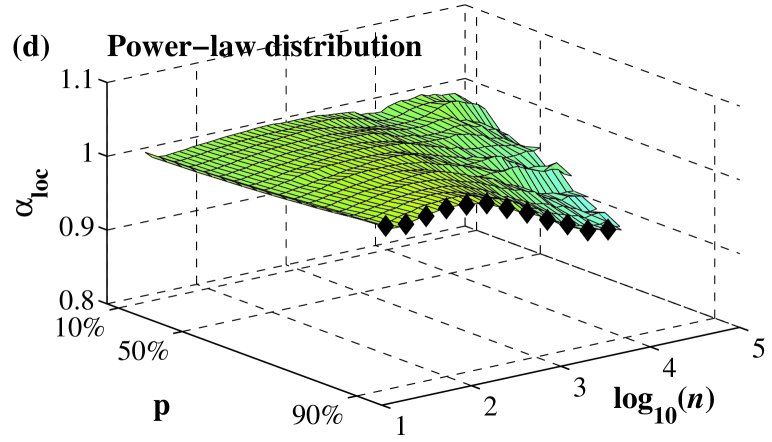
Figure 11: (Color online) Effect of the percentage $p$ of data loss on the local scaling behavior in long-range correlated signal with $\alpha=1.0$. The length of the data loss segments are (a) exponentially distributed, (b) Gaussian distributed, (c) $\delta$-distributed and (d) power-law distributed. In all the cases, the average length of removed segments $\mu=100$, and the length of the original signals $N=2^{20}$. Similar to Fig. 10, the exponential, Gaussian and $\delta$-distributions show similar changes in $\alpha_{loc}$ with $p$, while the power-law distribution shows less variations. The local scaling curves highlighted by black symbols correspond to the curves shown in Fig. 9.

III.3 Properties of remaining data segments: Effect of data loss on local scaling

In the previous section, we tested the effect of data loss by specifying the distribution and average length of removed segments. In this section, we study the effect of data loss by specifying the distribution and average length of remaining data segments. The results obtained by focusing on the properties of remaining data segments are different from what was shown above and will lead to a better understanding of the effect of data loss on the scaling behavior of long-range correlated signals.

The approach to generate the appropriate surrogate signals with different properties of remaining data segments is similar to the one described in Sec. II.3, except that now the binary series $g(i)$ are obtained according to the parameters of the remaining data segments, and the surrogate signals $\tilde{u}(i)$ are generated by removing the $i$-th data point in the original signal $u(i)$ if $g(i)=1$, and preserving the $i$-th data point if $g(i)=0$. The relation between the average length of data loss segments ($\mu_{l}$) and remaining data segments ($\mu_{r}$) can be derived as follows:

Let the length of the original signal be $N$. If $p_{l}$ is the percentage of data loss, the amount of data loss is given by $N_{l}=p_{l}N$, and the amount of remaining data is given by $N_{r}=p_{r}N=(1-p_{l})N$. If $\mu_{l}$ is the average length of the lost data segments, the number of lost segments is approximately given by $n_{l}~{}\approx~{}N_{l}/\mu_{l}$. The number of remaining data segments is approximately equal to the number of data loss segments, i.e., $n_{r}~{}\approx~{}n_{l}$. Hence, the average length of the remaining data segments is:

$$\mu_{r}~{}\approx~{}\frac{N_{r}}{n_{r}}~{}\approx~{}\frac{(1-p_{l})}{p_{l}}\mu_{l}.$$ (10)

Note that the lengths of data loss segments are always geometrically distributed due to the shuffling procedure in our segmentation approach (see Sec. II.3 and Fig. 12).

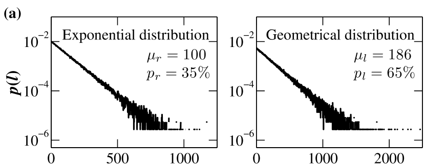
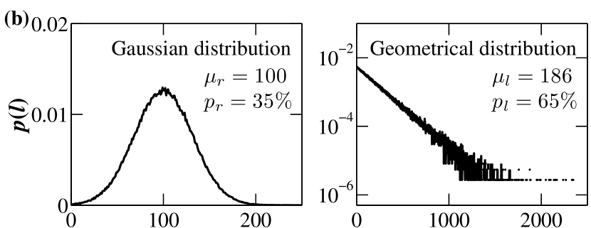
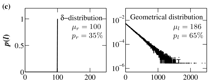
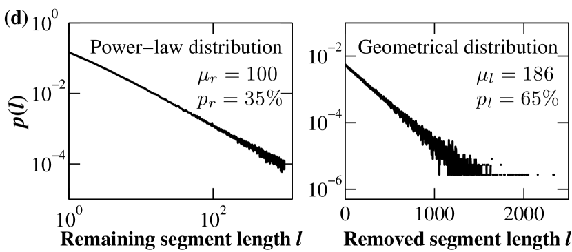
Figure 12: The distributions of remaining data segments (left column) and corresponding distributions of data loss segments (right column). The remaining data segments follow (a) exponential, (b) power-law, (c) Gaussian, and (d) $\delta$-distribution with average length $\mu_{r}$=100 and 35% of data remaining. The data loss segments are always geometrically distributed independent of the distributions of remaining segments. Note that, the average lengths are practically the same as estimated from Eq. 10.

We find similar changes in the scaling behavior as observed in Fig. 7 where the distribution of removed segment lengths was specified. As illustrated in Fig. 13 where the lengths of remaining segments are exponentially distributed, the local scaling behavior of anti-correlated surrogate signals deviate monotonically from original behavior towards uncorrelation at larger scales. While the local scaling exponents of positively correlated surrogate signals vary across scales, showing both overestimated and underestimated regions. These regions as well as the scales at which the anti-correlated signals reach $\alpha_{loc}=0.5$ are also shifted towards larger scales when the average length of remaining segments $\mu_{r}$ increases. However, in contrast to what was observed in Fig. 7, there is no shift to smaller scales with increasing percentage of data loss. Note that, according to Eq. 10, an average length $\mu_{r}=10$ of remaining segments and a percentage $p_{r}=10\%$ of remaining data (as shown in Fig. 13c), corresponds to an average length $\mu_{l}=90$ of removed segments and a percentage $p_{l}=90\%$ of removed data. Thus the local scaling behavior observed in Fig. 13c is vary similar to Fig. 7g (where $\mu_{l}=100$ and $p_{l}=90\%$), and Fig. 13d ($\mu_{r}=100$, $p_{r}=90\%$, $\mu_{l}=11$) is similar to Fig. 7a ($\mu_{l}=10$, $p_{l}=10\%$).

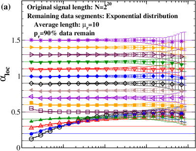
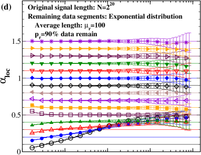
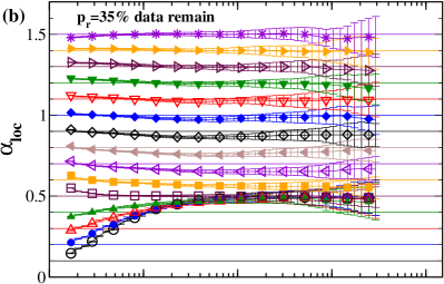
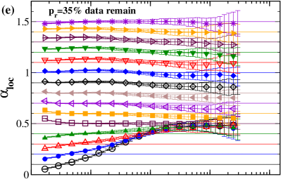
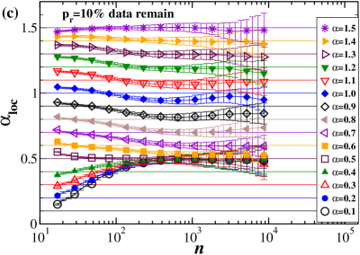
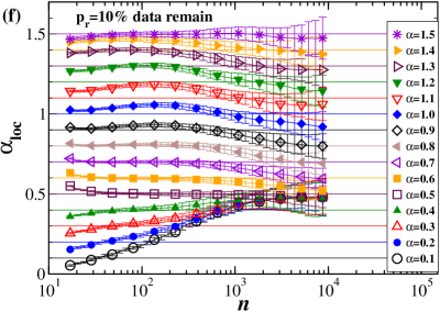
Figure 13: (Color online) Effect of data loss on the local scaling behavior of long-range correlated signals. The lengths of the remaining data segments are exponentially distributed with average length $\mu_{r}=10$ ((a)-(c)) and $\mu_{r}=100$ ((d)-(f)). The symbols indicate average $\alpha_{loc}$ values obtained from 100 different realizations of surrogate signals with the same correlation exponent $\alpha$, and the error bars show the standard deviations. The more data are removed, the more the scaling exponent deviates from the original exponent. For anti-correlated signals, the removal of larger segments ($\mu_{r}=100$) has less effect on the scaling behavior. For positively correlated signals, the deviations vary across scales, showing both overestimated and underestimated regions.

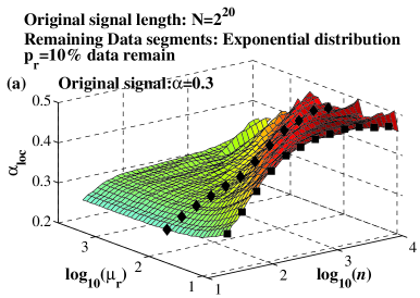
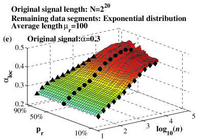
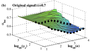
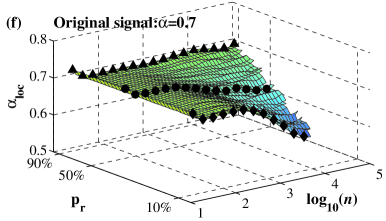
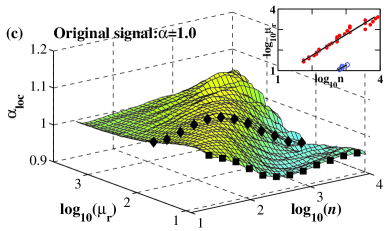
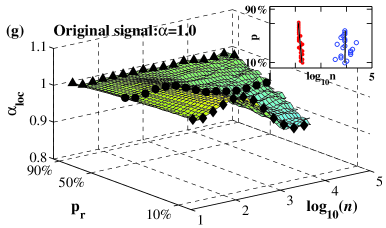
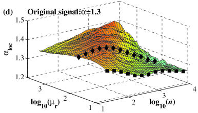
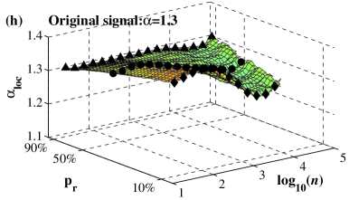
Figure 14: (Color online) Effect of the average length $\mu_{r}$ of remaining data segments (a)-(d) and effect of the percentage $p_{r}$ of remaining data (e)-(h) on the local scaling behavior in anti-correlated signals [(a), (e): $\alpha=0.3$] and positively correlated signals [(b), (f): $\alpha=0.7$; (c), (g): $\alpha=1.0$; (d), (h): $\alpha=1.3$]. For (a)-(d), $p_{r}=10\%$ of data are remained, and for (e)-(h), the average length of remaining segments $\mu_{r}=100$. In all the cases, the remaining segments are exponentially distributed, and the length of the original signals $N=2^{20}$. The symbols in the inset figures in (c) and (g) indicate the positions where $\alpha_{loc}$ values reach a maximum (red closed circle) and a minimum (blue open circle), which show that the overestimated and underestimated regions are shifted to larger scales only with increasing $\mu_{r}$ and are not shifted with the percentage $p_{r}$ of remaining data changes. The local scaling curves highlighted by black symbols correspond to the curves shown in Fig. 13 (rectangle: $\mu_{r}=10$, $p_{r}=10\%$; diamond: $\mu_{r}=100$, $p_{r}=10\%$; circle: $\mu_{r}=100$, $p_{r}=35\%$; triangle: $\mu_{r}=100$; $p_{r}=90\%$).

In Fig. 14a-d, we show how the local scaling behavior changes with the average length $\mu_{r}$ of remaining segments. Similar to Fig. 8a-d where the distribution of removed segments was specified, the variation of the local scaling behavior of positively correlated signals also shows overestimated regions at smaller scales followed by underestimated regions at larger scales. Both regions are shifted to larger scales, when the average length of remaining segments increases, forming a power-law relationship between the shift in the local scaling behavior and $\mu_{r}$ (Fig. 14c). For anti-correlated signals the local scaling behavior also shows a power-law relationship between the scale at which $\alpha_{loc}$ reaches 0.5 and the average length $\mu_{r}$. Note that, according to Eq. 10, the $\alpha_{loc}$ curves from $\mu_{r}$=8 to 455 in Fig. 14a-d correspond to $\mu_{l}$=72 to 4095 in Fig. 8a-d, thus the local scaling behavior in these two regions are very similar.

With increasing percentage $p_{r}$ of remaining data, the deviation from the original scaling behavior becomes smaller (Fig. 14e-h). However, for anti-correlated signals, the scale at which $\alpha_{loc}$ reaches 0.5 does not depend on the percentage of data loss (Fig. 14e), in contrast to Fig. 8e where removed data segments were studied. Similarly, the overestimated regions in positively correlated signals are also not shifted with the percentage of data loss (Fig. 14f-h, and compare to Fig. 8f-h).

Next, we investigate how different kinds of distributions of remaining data segments influence the local scaling behavior. As illustrate in Fig. 15, the surrogate signals generated by using Gaussian or $\delta$-distribution have almost identical local scaling behavior and the most pronounced deviation from the original local scaling behavior, and the power-law distribution shows the smallest deviations. Note that, the local scaling exponent of surrogate signals generated by a $\delta$-distribution jump to larger $\alpha_{loc}$ values at certain small scales when the scaling exponent of the original signal is 1.3, 1.4 and 1.5. This behavior is caused by the discontinuities in the surrogate signal at the transition points between remaining data segments, and since the remaining segments are of fixed length, the transition points occur periodically. If the segment length ($\mu=100$ in Fig. 15) is an integral multiple of the size of the fitting boxes (scales) in the DFA algorithm (e.g., $n=10,20,25,50$), the transition points are not included in any fitting box and thus the rms fluctuation functions of the surrogate signals will be the same as in the original signals. In all other cases, the discontinuities inside the fitting box will cause larger rms fluctuation functions and lead to jumps in the local scaling exponents at certain scales $n\leq\mu_{r}$ as observed in Fig. 15.

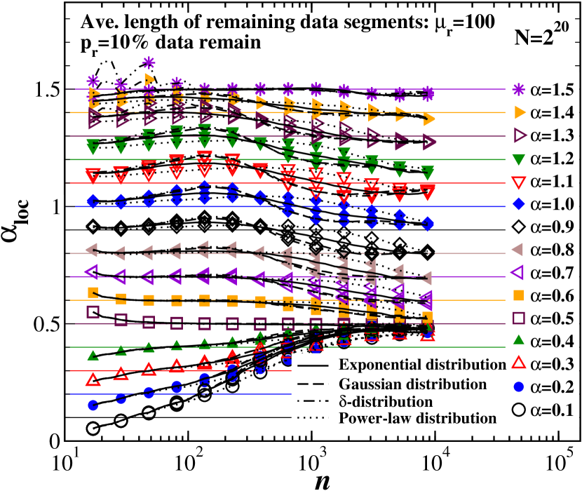
Figure 15: Effect of different kinds of distributions of remaining data segments on the local scaling behavior. The Gaussian and $\delta$-distributions lead to identical and most pronounced deviations from the original scaling behavior for both anti-correlated and positively correlated signals. The power-law distribution leads to lowest deviations for anti-correlated signals and a smoother behavior of $\alpha_{loc}$ versus $\mu_{r}$, i.e., a less pronounced over- and underestimation of the original scaling behavior for positively correlated signals. Interestingly, for positively correlated signals, all four kinds of distributions yield the same local scaling exponent $\alpha_{loc}$ at certain scale ($n~{}\approx~{}300$ for $\mu_{r}=100$). Note that in case of the $\delta$-distribution, large jumps of $\alpha_{loc}$ values at small scales occur for original scaling exponents $\alpha=$1.3 to 1.5 (see text for more details).

In Fig. 16, we show how the local scaling curves of positively correlated signals change with the average length $\mu_{r}$ of remaining segments, which follow an exponential distribution (Fig. 16a), a Gaussian distribution (Fig. 16b), a $\delta$-distribution (Fig. 16c), and a power-law distribution (Fig. 16d). The Gaussian and $\delta$-distributions lead to a similar local scaling behavior with regions of pronounced overestimation and underestimation which are shifted to larger scales for increasing values of $\mu_{r}$. This shift is also observed in the case of the exponential distribution, however, the deviation from the original scaling behavior (overestimation/underestimation) is less pronounced. In contrast, the power-law distribution shows less variation of the local scaling behavior and does not lead to such distinct regions of over- and underestimated $\alpha_{loc}$ values. In addition, the local scaling curves do not show a clear dependency (“shift”) with the average length of remaining segments $\mu_{r}$.

The variation of the local scaling curves with the percentage $p_{r}$ of remaining data for the four different distributions are presented in Fig. 17. Similar as shown in Fig. 14, the scale of most pronounced deviation from the original scaling behavior is independent of the percentage $p_{r}$ of remaining data.

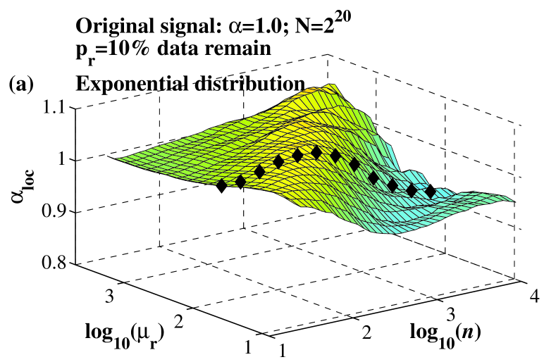
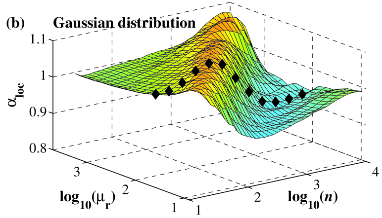
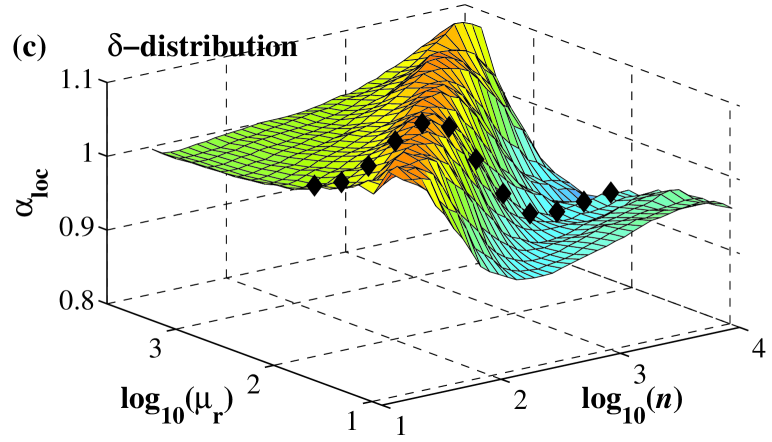
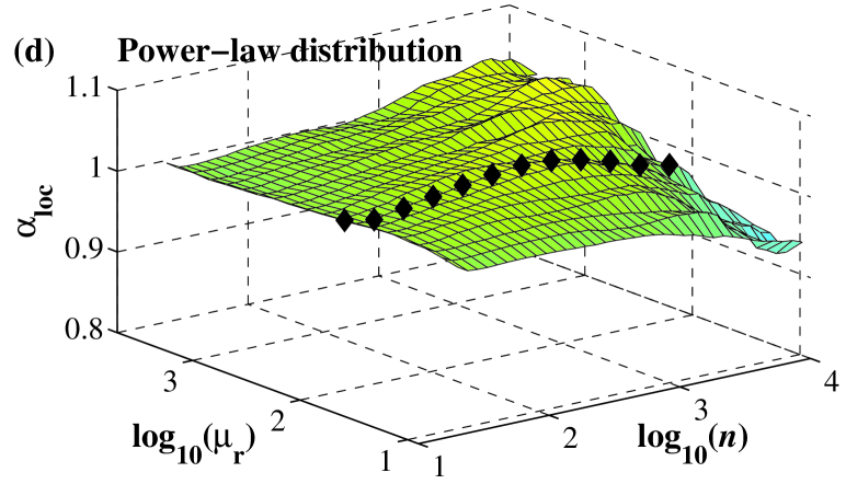
Figure 16: Effect of different distributions and the average length $\mu_{r}$ of remaining data segments on the local scaling behavior. In all the cases, $p_{r}=10\%$ of data are remained, and the length of the original signals $N=2^{20}$. The Gaussian and $\delta$-distribution lead to very similar behavior with most pronounced $\alpha_{loc}$ deviations and a clear shift with $\mu_{r}$. In contrast, the power-law distribution shows no clear dependency of $\alpha_{loc}$ with $\mu_{r}$. The local scaling curves highlighted by black symbols correspond to the curves shown in Fig. 15.

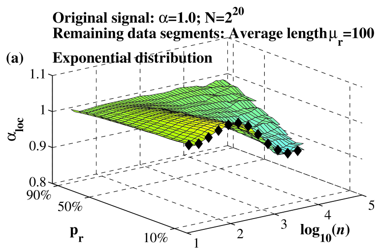
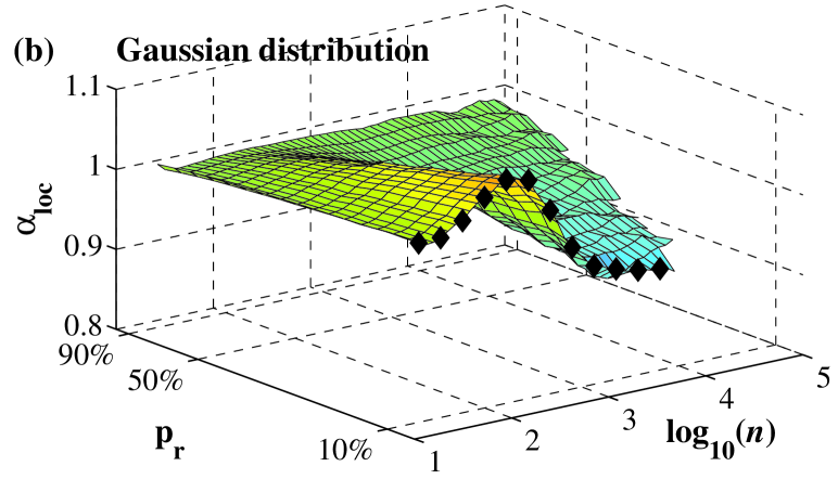
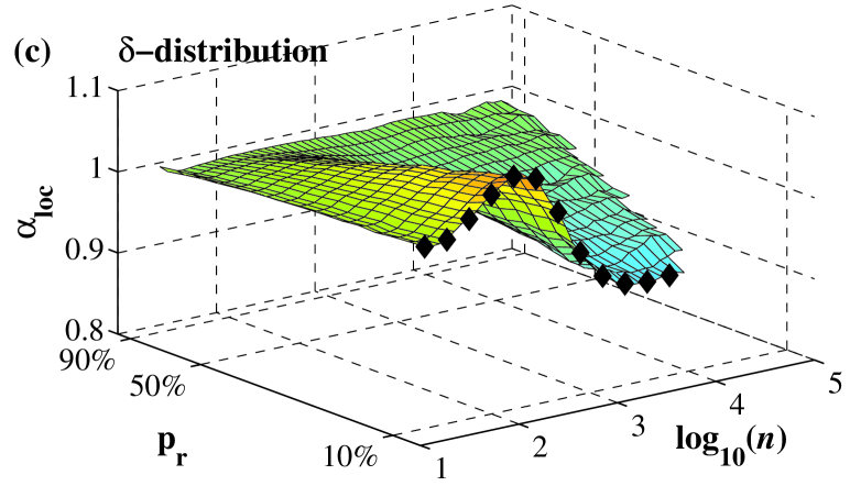
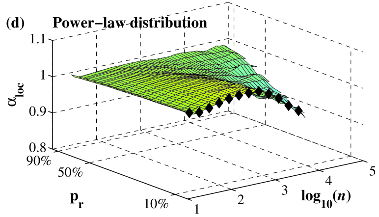
Figure 17: Effect of different distributions of remaining data segments and the percentage $p_{r}$ of remaining data on the local scaling behavior. In all the cases, the average length of remaining segments $\mu_{r}=100$, and the length of the original signals $N=2^{20}$. The deviations from original scaling behavior are more pronounced for smaller percentages of remaining data. Note that the scale at which the most pronounced deviation is observed does not depend on $p_{r}$. The local scaling curves highlighted by black symbols correspond to the curves shown in Fig. 15.

IV Summary and Conclusion

In this paper, we studied the effect of extreme data loss on the DFA scaling behavior of long-range power-law correlated signals. In order to simulate extreme data loss, often encountered in archaeological and geological data, we developed a new segmentation approach to generate correlated signals with randomly removed data segments. Using this approach, surrogate signals can be generated for different percentages of data loss, different average lengths and different distributions of removed/remaining data segments. We compared the difference between the DFA scaling behavior of original and surrogate signals by systematically changing the percentage of data loss and the average length of removed/remaining segments, and we also consider different functional forms of the distributions of removed/remaining segment lengths. We studied changes in the global scaling behavior as well as in the local scaling exponents to reveal subtle deviations across scales.

We find that anti-correlated signals are very sensitive to data loss. Even if only 10% of the data are removed, the scaling behavior of the surrogate signals changes dramatically, showing uncorrelated behavior at large scales. In contrast, positively correlated signals are more robust to data loss and no significant changes in the global scaling behavior are observed for up to 90% of data loss. However, in case of extreme data loss, we find significant and systematic deviations in the local scaling behavior which is overestimated at small scales and underestimated at large scales. Specifically, we find that for anti-correlated signals the scale at which the local scaling exponent $\alpha_{loc}$ reaches 0.5 shifts to larger scales with increasing the average length $\mu_{l}$ (or $\mu_{r}$) of the removed (or remaining) segments, following a power-law relationship with $\mu_{l}$ (or $\mu_{r}$). For positively correlated signals the regions of overestimation and underestimation of the local scaling exponent are also shifted to larger scales following a power-law with increasing $\mu_{l}$ (or $\mu_{r}$).

As expected, increasing the percentage of data loss leads to more pronounced deviations in the local scaling behavior. However, the variation of local scaling curves follows different rules if the properties of either removed segments or remaining segments are considered. When the average length $\mu_{l}$ of removed data segments is kept constant, for increasing percentage $p_{l}$ of removed data, the deviations of both anti-correlated and positively correlated signals are shifted to smaller scales following a power-law with $p_{l}$. When we focus on remaining data segments and keep their average length $\mu_{r}$ constant, the deviations become more pronounced with decreasing percentage $p_{r}$ of remaining data, however, the deviations occur at the same scales.

This behavior can be explained by the relationship between removed and remaining data. In case of a fixed percentage of removed or remaining data, $\mu_{l}$ and $\mu_{r}$ are always directly proportional to each other (Eq. 10) and therefore the deviations (and the shift of the most pronounced deviation) show a similar power-law relation with $\mu_{l}$ and $\mu_{r}$, while fixing the average length of removed or remaining segments leads to two different scenarios: (i) fixing $\mu_{l}$ and changing $p_{l}$ leads to changes in $\mu_{r}$ proportional to $p_{l}$; (ii) fixing $\mu_{r}$ and changing $p_{r}$ leads to changes in $\mu_{l}$ proportional to $p_{r}$. Since the scale of the most pronounced deviation from the original scaling behavior is shifted for scenario (i) where $\mu_{r}$ is changing and $\mu_{l}$ is fixed, but not scenario (ii) where $\mu_{l}$ is changing and $\mu_{r}$ is fixed, changes in $\mu_{l}$ do not contribute to the observed shift. Thus, we suggest that $\mu_{r}$ is the key parameter to determine the scales at which the scaling behavior is mostly influenced, whereas the percentage of data loss determines the extent of this influence.

Different distributions of the lengths of removed/remaining segments affect the local scaling behavior differently. For Gaussian and $\delta$-distributed segment lengths, deviations are most pronounced and similar in extent, whereas power-law distributed segments show smallest deviations and a very different overall behavior when compare to exponential, Gaussian and $\delta$-distributed segments.

In conclusion, our study shows that it is important to consider not only the percentage of data loss (removed/remaining data), but also the average length of remaining segments to identify the scales at which deviations from the original (“real”) DFA scaling behavior is most pronounced. Therefore, when studying the scaling properties of signals with extreme data loss, the DFA results should be carefully interpreted to reveal the real scaling behavior.

References

- Stanley (1995) H. E. Stanley, Nature 378, 554 (1995).
- Shlesinger (1987) M. F. Shlesinger, Ann N Y Acad Sci 504, 214 (1987).
- Liebovitch (1994) L. S. Liebovitch, Adv Chem Ser 235, 357 (1994).
- Ivanov et al. (1998) P. Ch. Ivanov, L. A. N. Amaral, A. L. Goldberger, and H. E. Stanley, Europhys Lett 43, 363 (1998).
- Ashkenazy et al. (2002) Y. Ashkenazy, J. Hausdorff, P. Ch. Ivanov, and H. E. Stanley, Physica A 316, 662 (2002).
- Bassingthwaighte et al. (1994) J. B. Bassingthwaighte, L. Liebovitch, and B. J. West, Fractal Physiology. (Oxford University Press, 1994).
- Malik and Camm (1995) M. Malik and A. Camm, Heart Rate Variability. (Futura, Armonk NY, 1995).
- Hurst (1951) H. E. Hurst, Trans Am Soc Civ Eng 116, 770 (1951).
- Mandelbrot and Wallis (1969) B. B. Mandelbrot and J. R. Wallis, Water Resources Research 5, 321 (1969).
- Stratonovich (1981) R. L. Stratonovich, Topics in the Theory of Random Noise, vol. I. (Gordon and Breach, New York, 1981).
- Peng et al. (1994) C.-K. Peng, S. V. Buldyrev, S. Havlin, M. Simons, H. E. Stanley, and A. L. Goldberger, Phys. Rev. E 49, 1685 (1994).
- Taqqu et al. (1995) M. Taqqu, V. Teverovsky, and W. Willinger, Fractals 3, 785 (1995).
- Peng et al. (1992) C.-K. Peng, S. V. Buldyrev, A. L. Goldberger, S. Havlin, F. Sciortino, M. Simons, and H. E. Stanley, Nature 356, 168 (1992).
- Peng et al. (1993) C.-K. Peng, S. V. Buldyrev, A. L. Goldberger, S. Havlin, M. Simons, and H. E. Stanley, Phys. Rev. E 47, 3730 (1993).
- Buldyrev et al. (1993) S. V. Buldyrev, A. L. Goldberger, S. Havlin, C.-K. Peng, H. E. Stanley, and M. Simons, Biophys. J. 65, 2673 (1993).
- Ossadnik et al. (1994) S. M. Ossadnik, S. B. Buldyrev, A. L. Goldberger, S. Havlin, R. N. Mantegna, C.-K. Peng, M. Simons, and H. E. Stanley, Biophys. J. 67, 64 (1994).
- Stanley et al. (1994) H. E. Stanley, S. V. Buldyrev, A. L. Goldberger, S. Havlin, R. N. Mantegna, C.-K. Peng, and M. Simons, Nuovo Cimento Soc. Ital. Fis. D 16, 1339 (1994).
- Mantegna et al. (1994) R. N. Mantegna, S. V. Buldyrev, A. L. Goldberger, S. Havlin, C.-K. Peng, M. Simons, and H. E. Stanley, Phys. Rev. Lett. 73, 3169 (1994).
- Havlin et al. (1995a) S. Havlin, S. V. Buldyrev, A. L. Goldberger, R. N. Mantegna, S. M. Ossadnik, C.-K. Peng, M. Simon, and H. E. Stanley, Chaos Soliton Fract. 6, 171 (1995a).
- Peng et al. (1995a) C.-K. Peng, S. V. Buldyrev, A. L. Goldberger, S. Havlin, R. N. Mantegna, M. Simons, and H. E. Stanley, Physica A 221, 180 (1995a).
- Havlin et al. (1995b) S. Havlin, S. V. Buldyrev, A. L. Goldberger, R. N. Mantegna, C.-K. Peng, M. Simons, and H. E. Stanley, Fractals 3, 269 (1995b).
- Mantegna et al. (1996) R. N. Mantegna, S. V. Buldyrev, A. L. Goldberger, S. Havlin, C.-K. Peng, M. Simons, and H. E. Stanley, Phys. Rev. Lett. 76, 1979 (1996).
- Buldyrev et al. (1998) S. V. Buldyrev, N. V. Dokholyan, A. L. Goldberger, S. Havlin, C.-K. Peng, H. E. Stanley, and G. M. Viswanathan, Physica A 249, 430 (1998).
- Stanley et al. (1999) H. E. Stanley, S. V. Buldyrev, A. L. Goldberger, S. Havlin, C.-K. Peng, and M. Simons, Physica A 273, 1 (1999).
- Li et al. (2003) W. Li, P. Bernaola-Galvan, P. Carpena, and J. L. Oliver, Comput. Biol. Chem. 27, 5 (2003).
- Hackenberg et al. (2005) M. Hackenberg, P. Bernaola-Galvan, P. Carpena, and J. L. Oliver, J. Mol. Evol. 60, 365 (2005).
- Peng et al. (1995b) C.-K. Peng, S. Havlin, H. E. Stanley, and A. L. Goldberger, Chaos 5, 82 (1995b).
- Ho et al. (1997) K. K. L. Ho, G. B. Moody, C.-K. Peng, J. E. Mietus, M. G. Larson, D. Levy, and A. L. Goldberger, Circulation 96, 842 (1997).
- Barbi et al. (1998) M. Barbi, S. Chillemi, A. Di Garbo, R. Balocchi, C. Carpeggiani, M. Emdin, C. Michelassi, and E. Santarcangelo, Chaos Soliton Fract. 9, 507 (1998).
- Ivanov et al. (1999) P. Ch. Ivanov, A. Bunde, L. A. N. Amaral, S. Havlin, J. Fritsch-Yelle, R. M. Baevsky, H. E. Stanley, and A. L. Goldberger, Europhys. Lett. 48, 594 (1999).
- Pikkujämsä et al. (1999) S. M. Pikkujämsä, T. H. Mäkikallio, L. B. Sourander, I. J. Räihä, P. Puukka, J. Skyttä, C.-K. Peng, A. L. Goldberger, and H. V. Huikuri, Circulation 100, 393 (1999).
- Ashkenazy et al. (1999) Y. Ashkenazy, M. Lewkowicz, J. Levitan, S. Havlin, K. Saermark, H. Moelgaard, and P. E. B. Thomsen, Fractals 7, 85 (1999).
- Absil et al. (1999) P. A. Absil, R. Sepulchre, A. Bilge, and P. Gerard, Physica A 272, 235 (1999).
- Toweill et al. (2000) D. Toweill, K. Sonnenthal, B. Kimberly, S. Lai, and B. Goldstein, Crit. Care Med. 28, 2051 (2000).
- Bunde et al. (2000) A. Bunde, S. Havlin, J. W. Kantelhardt, T. Penzel, J.-H. Peter, and K. Voigt, Phys. Rev. Lett. 85, 3736 (2000).
- Laitio et al. (2000) T. Laitio, H. Huikuri, E. Kentala, T. Makikallio, J. Jalonen, H. Helenius, K. Sariola-Heinonen, S. Yli-Mayry, and H. Scheinin, Anesthesiology 93, 69 (2000).
- Ashkenazy et al. (2000) Y. Ashkenazy, P. Ch. Ivanov, S. Havlin, C.-K. Peng, Y. Yamamoto, A. L. Goldberger, and H. E. Stanley, Comput. Cardiol. 27, 139 (2000).
- Ashkenazy et al. (2001) Y. Ashkenazy, P. Ch. Ivanov, S. Havlin, C.-K. Peng, A. L. Goldberger, and H. E. Stanley, Phys. Rev. Lett. 86, 1900 (2001).
- Ivanov et al. (2001) P. Ch. Ivanov, L. A. N. Amaral, A. L. Goldberger, S. Havlin, M. G. Rosenblum, H. E. Stanley, and Z. Struzik, Chaos 11, 641 (2001).
- Kantelhardt et al. (2002) J. W. Kantelhardt, Y. Ashkenazy, P. Ch. Ivanov, A. Bunde, S. Havlin, T. Penzel, J.-H. Peter, and H. E. Stanley, Phys. Rev. E 65, 051908 (2002).
- Karasik et al. (2002) R. Karasik, N. Sapir, Y. Ashkenazy, P. Ch. Ivanov, I. Dvir, P. Lavie, and S. Havlin, Phys. Rev. E 66, 062902 (2002).
- Ivanov et al. (2004a) P. Ch. Ivanov, Z. Chen, K. Hu, and H. E. Stanley, Physica A 344, 685 (2004a).
- Bartsch et al. (2005) R. Bartsch, T. Hennig, A. Heinen, S. Heinrichs, and P. Maass, Physica A 354, 415 (2005).
- Schmitt and Ivanov (2007) D. T. Schmitt and P. Ch. Ivanov, Am. J. Physiol.-Regul. Integr. Comp. Physiol. 293, R1923 (2007).
- Schmitt et al. (2009) D. T. Schmitt, P. K. Stein, and P. Ch. Ivanov, IEEE Trans. Biomed. Eng. 56, 1564 (2009).
- Mäkikallio et al. (1999) T. H. Mäkikallio, J. Koistinen, L. Jordaens, M. P. Tulppo, N. Wood, B. Golosarsky, C.-K. Peng, A. L. Goldberger, and H. V. Huikuri, T Am J Cardiol 83, 880 (1999).
- Hausdorff et al. (1995) J. M. Hausdorff, C.-K. Peng, Z. Ladin, J. Y. Wei, and A. L. Goldberger, J. Appl. Physiol. 78, 349 (1995).
- Bartsch et al. (2007) R. Bartsch, M. Plotnik, J. W. Kantelhardt, S. Havlin, N. Giladi, and J. M. Hausdorff, Physica A 383, 455 (2007).
- Ivanov et al. (2009) P. Ch. Ivanov, Q. D. Y. Ma, R. P. Bartsch, J. M. Hausdorff, L. A. N. Amaral, V. Schulte-Frohlinde, H. E. Stanley, and M. Yoneyama, Phys. Rev. E 79, 041920 (2009).
- Hu et al. (2004) K. Hu, P. Ch. Ivanov, Z. Chen, M. F. Hilton, H. E. Stanley, and S. A. Shea, Physica A 337, 307 (2004).
- Ivanov et al. (2007) P. Ch. Ivanov, K. Hu, M. F. Hilton, S. A. Shea, and H. E. Stanley, Proc. Natl. Acad. Sci. USA 104, 20702 (2007).
- Ivanov (2007) P. Ch. Ivanov, IEEE Eng. Med. Biol. 26, 33 (2007).
- Hu et al. (2007) K. Hu, F. A. J. L. Scheer, P. Ch. Ivanov, R. M. Buijs, and S. A. Shea, Neuroscience 149, 508 (2007).
- Bahar et al. (2001) S. Bahar, J. Kantelhardt, A. Neiman, H. Rego, D. Russell, L. Wilkens, A. Bunde, and F. Moss, Europhys. Lett. 56, 454 (2001).
- Varotsos et al. (2003) P. A. Varotsos, N. V. Sarlis, and E. S. Skordas, Phys. Rev. E 67, 021109 (2003).
- Varotsos et al. (2009) P. A. Varotsos, N. V. Sarlis, and E. S. Skordas, Chaos 19, 023114 (2009).
- Ivanova and Ausloos (1999) K. Ivanova and M. Ausloos, Physica A 274, 349 (1999).
- Koscielny-Bunde et al. (1998a) E. Koscielny-Bunde, A. Bunde, S. Havlin, H. E. Roman, Y. Goldreich, and H.-J. Schellnhuber, Phys. Rev. Lett. 81, 729 (1998a).
- Koscielny-Bunde et al. (1998b) E. Koscielny-Bunde, H. Roman, A. Bunde, S. Havlin, and H. Schellnhuber, Philos. Mag. B 77, 1331 (1998b).
- Talkner and Weber (2000) P. Talkner and R. Weber, Phys. Rev. E 62, 150 (2000).
- Bunde et al. (2001) A. Bunde, S. Havlin, E. Koscielny-Bunde, and H.-J. Schellnhuber, Physica A 302, 255 (2001).
- Monetti et al. (2003) R. A. Monetti, S. Havlin, and A. Bunde, Physica A 320, 581 (2003).
- Bunde et al. (2005) A. Bunde, J. F. Eichner, J. W. Kantelhardt, and S. Havlin, Phys. Rev. Lett. 94, 048701 (2005).
- Montanari et al. (2000) A. Montanari, R. Rosso, and M. S. Taqqu, Water Resour. Res. 36, 1249 (2000).
- Matsoukas et al. (2000) C. Matsoukas, S. Islam, and I. Rodriguez-Iturbe, J. Geophys. Res. 105, 29165 (2000).
- Liu et al. (1997) Y. H. Liu, P. Cizeau, M. Meyer, C.-K. Peng, and H. E. Stanley, Physica A 245, 437 (1997).
- Vandewalle and Ausloos (1997) N. Vandewalle and M. Ausloos, Physica A 246, 454 (1997).
- Vandewalle and Ausloos (1998) N. Vandewalle and M. Ausloos, Phys. Rev. E 58, 6832 (1998).
- Liu et al. (1999) Y. Liu, P. Gopikrishnan, P. Cizeau, M. Meyer, C.-K. Peng, and H. E. Stanley, Phys. Rev. E 60, 1390 (1999).
- Janosi et al. (1999) I. M. Janosi, B. Janecsko, and I. Kondor, Physica A 269, 111 (1999).
- Ausloos et al. (1999) M. Ausloos, N. Vandewalle, P. Boveroux, A. Minguet, and K. Ivanova, Physica A 274, 229 (1999).
- Roberto et al. (1999) M. Roberto, E. Scalas, G. Cuniberti, and M. Riani, Physica A 269, 148 (1999).
- Vandewalle et al. (1999) N. Vandewalle, M. Ausloos, and P. Boveroux, Physica A 269, 170 (1999).
- Grau-Carles (2000) P. Grau-Carles, Physica A 287, 396 (2000).
- Ausloos (2000) M. Ausloos, Physica A 285, 48 (2000).
- Ausloos and Ivanova (2000) M. Ausloos and K. Ivanova, Physica A 286, 353 (2000).
- Ausloos and Ivanova (2001a) M. Ausloos and K. Ivanova, Phys. Rev. E 63, 047201 (2001a).
- Ausloos and Ivanova (2001b) M. Ausloos and K. Ivanova, Int. J. Mod. Phys. C 12, 169 (2001b).
- Ivanov et al. (2004b) P. Ch. Ivanov, A. Yuen, B. Podobnik, and Y. Lee, Phys. Rev. E 69, 056107 (2004b).
- Metzner et al. (2007) C. Metzner, C. Raupach, D. Paranhos Zitterbart, and B. Fabry, Phys. Rev. E 76, 021925 (2007).
- Kantelhardt et al. (2003) J. W. Kantelhardt, S. Havlin, and P. Ch. Ivanov, Europhys Lett 62, 147 (2003).
- Hu et al. (2001) K. Hu, P. Ch. Ivanov, Z. Chen, P. Carpena, and H. E. Stanley, Phys. Rev. E 64, 011114 (2001).
- Chen et al. (2002) Z. Chen, P. Ch. Ivanov, K. Hu, and H. E. Stanley, Phys. Rev. E 65, 041107 (2002).
- Chen et al. (2005) Z. Chen, K. Hu, P. Carpena, P. Bernaola-Galvan, H. E. Stanley, and P. Ch. Ivanov, Phys. Rev. E 71, 011104 (2005).
- Xu et al. (2005) L. Xu, P. Ch. Ivanov, K. Hu, Z. Chen, A. Carbone, and H. E. Stanley, Phys. Rev. E 71, 051101 (2005).
- Alvarez-Ramirez et al. (2005) J. Alvarez-Ramirez, E. Rodriguez, and J. Echeverria, Physica A 354, 199 (2005).
- Nagarajan (2006) R. Nagarajan, Physica A 363, 226 (2006).
- Bashan et al. (2008) A. Bashan, R. Bartsch, J. W. Kantelhardt, and S. Havlin, Physica A 387, 5080 (2008).
- Kantelhardt et al. (2001) J. W. Kantelhardt, E. Koscielny-Bunde, H. H. Rego, S. Havlin, and A. Bunde, Physica A 295, 441 (2001).
- Makse et al. (1996) H. A. Makse, S. Havlin, M. Schwartz, and H. E. Stanley, Phys. Rev. E 53, 5445 (1996).
- Temin (2002) P. Temin, Explorations in Economic History 39, 46 (2002).