Farthest-Polygon Voronoi Diagrams

Abstract

Given a family of $k$ disjoint connected polygonal sites in general position and of total complexity $n$, we consider the farthest-site Voronoi diagram of these sites, where the distance to a site is the distance to a closest point on it. We show that the complexity of this diagram is $O(n)$, and give an $O(n\log^{3}n)$ time algorithm to compute it. We also prove a number of structural properties of this diagram. In particular, a Voronoi region may consist of $k-1$ connected components, but if one component is bounded, then it is equal to the entire region.

1 Introduction

Consider a family $\mathcal{S}$ of geometric objects, called sites, in the plane. The farthest-site Voronoi diagram of $\mathcal{S}$ subdivides the plane into regions, each region associated with one site $P\in\mathcal{S}$, and containing those points $x\in\mathbb{R}^{2}$ for which $P$ is the farthest among the sites of $\mathcal{S}$.

While closest-site Voronoi diagrams have been studied extensively [4], their farthest-site cousins have received somewhat less attention. For the case of (possibly intersecting) line segment sites, Aurenhammer et al. [3] recently presented an $O(n\log n)$ time algorithm to compute their farthest-site diagram.

Farthest-site Voronoi diagrams have a number of important applications. Perhaps the most well-known one is the problem of finding a smallest disk that intersects all the sites [1]. This disk can be computed in linear time once the diagram is known, since its center is a vertex or lies on an edge of the diagram. Another standard application is to build a data structure to quickly report the site farthest from a given query point.

We are here interested in the case of complex sites with non-constant description complexity. This setting was perhaps first considered by Abellanas et al. [1]: their sites are finite point sets, and so the distance to a site is the distance to the nearest point of that site. Put differently, they consider $n$ points colored with $k$ different colors, and their farthest-color Voronoi diagram subdivides the plane depending on which color is farthest away. The motivation for this problem is the one mentioned above, namely to find a smallest disk that contains a point of each color—this is a facility location problem where the goal is to find a position that is as close as possible to each of $k$ different types of facilities (such as schools, post offices, supermarkets, etc.). In a companion paper [2] the authors study other color-spanning objects.

The farthest-color Voronoi diagram is easily seen to be the projection of the upper envelope of the $k$ Voronoi surfaces corresponding to the $k$ color classes. Huttenlocher et al. [11] show that this upper envelope has complexity $\Theta(nk)$ for $n$ points, and can be computed in time $O(nk\log n)$ (see also the book by Sharir and Agarwal [19, §8.7].

Van Kreveld and Schlechter [13] consider the farthest-site Voronoi diagram for a family of disjoint simple polygons. Again, they are interested in finding the center of the smallest disk intersecting or touching all polygons, which they then apply to the cartographic problem of labeling groups of islands. Their algorithm is based on the claim that this farthest-polygon Voronoi diagram is an instance of the abstract farthest-site Voronoi diagram defined by Mehlhorn et al. [15]—but this claim is false, since the bisector of two disjoint simple polygons can be a closed curve, see Fig. 1(a). In particular, Voronoi regions can be bounded (which is impossible for regions in abstract farthest-site Voronoi diagrams).

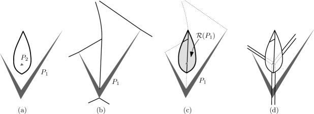
Figure 1: (a) The bisector of two polygons can be a closed curve. (b) The medial axis $\mathfrak{M}(P_{1})$ outside of $P_{1}$. (c) The Voronoi region $\mathcal{R}(P_{1})$, shown in light gray. (d) The farthest-polygon Voronoi diagram $\mathfrak{F}(\{P_{1},P_{2}\})$.

Note that the farthest-polygon Voronoi diagram can again be expressed as the upper envelope of $k$ Voronoi surfaces—but this does not seem to lead to anything stronger than near-quadratic complexity and time bounds.

We show in this paper that, in fact, the complexity of the farthest-polygon Voronoi diagram of $k$ disjoint simple polygons of total complexity $n$ is $O(n)$. We also show some structural properties of this diagram. In particular, Voronoi regions can be disconnected, and in fact, the region of a polygon $P$ can consist of up to $k-1$ connected components. However, if one connected component is bounded then it is equal to the entire region of $P$; moreover, the region is simply connected and the convex hull of $P$ contains another polygon in its interior. Furthermore, the Voronoi regions consist, in total, of at most $2k-2$ connected components, and this bound is tight.

Algorithms for computing closest-site Voronoi diagrams make use of the fact that Voronoi regions surround and are close to their sites. Similarly, algorithms for computing farthest-site Voronoi diagrams make use of the unboundedness of the Voronoi regions, and often build up regions from infinity [3]. The difficulty in computing farthest-polygon Voronoi diagrams is that neither of these properties holds: Voronoi regions can be bounded, and finding the location of these bounded regions is the bottleneck in the computation.

We give a divide-and-conquer algorithm with running time $O(n\log^{3}n)$ to compute the farthest-polygon Voronoi diagram. Our key idea is to build point location data structures for the partial diagrams already computed, and to use parametric search on these data structures to find suitable starting vertices for the merging step. This idea may find applications in the computation of other complicated Voronoi diagrams. Our algorithm implies an $O(n\log^{3}n)$ algorithm to compute the smallest disk touching or intersecting all the input polygons.

We note that for a family of disjoint convex polygons, finding the smallest disk touching all of them is much easier, and can be solved in time $O(n)$, where $n$ is the total complexity of the polygons [12].

In Section 2, we start with some preliminaries and give a definition of farthest-polygon Voronoi diagrams. We prove, in Section 3, some properties on the structure of these diagrams and bound their complexity. In Section 4, we present an algorithm for computing such diagrams and conclude in Section 5.

2 Preliminaries

We consider a family $\mathcal{S}$ of $k$ pairwise-disjoint polygonal sites of total complexity $n$. Here, a polygonal site of complexity $m$ is the union of $m$ line segments, whose relative interiors are pairwise disjoint, but whose union is connected, see Fig. 2. (In other words, the corners and edges of a polygonal site form a one-dimensional connected simplicial complex in the plane.) In particular, the boundary of a simple polygon is a polygonal site. For a point $x\in\mathbb{R}^{2}$, the distance $d(x,P)$ between $x$ and a site $P\in\mathcal{S}$ is the Euclidean distance from $x$ to the closest point on $P$.

A pocket $\mathcal{P}$ of $P$ is a connected component of $\operatorname{CH}(P)\setminus P$, where $\operatorname{CH}(P)$ is the convex hull of $P$. A pocket $\mathcal{P}$ is bounded if it coincides with a bounded connected component of $\mathbb{R}^{2}\setminus P$, unbounded otherwise.

The features of a site $P$ are its corners and edges. We say that a disk touches a corner if the corner lies on its boundary. A disk touches an edge if the closed edge touches the disk in one point and if its supporting line is tangent to the disk. A disk touches a site $P$ if the disk touches some of $P$’s features and if the disk’s interior does not intersect $P$.

Figure 2: A polygonal site $P$ with three bounded pockets and seven unbounded ones, and its convex hull. A point $x$ and the disk $D_{P}(x)$.

We assume that the family $\mathcal{S}$ is in general position, that is, no disk touches four features, no line contains three corners, and no two edges are parallel.

Before defining the farthest-polygon Voronoi diagram of a family of polygonal sites, we define the medial axis of a polygonal site.

Medial axes.

For a site $P\in\mathcal{S}$, we define the function $\Psi_{P}:\mathbb{R}^{2}\mapsto\mathbb{R}$ as $\Psi_{P}(x)=d(x,P)$. The graph of $\Psi_{P}$ is a Voronoi surface; it is the lower envelope of circular cones for each corner of $P$ and of rectangular wedges for each edge of $P$. The orthogonal projection of this surface on the plane induces a subdivision of the plane: each 2D cell of this subdivision corresponds to a feature $w$ of $P$, and it is the set of all points $x\in\mathbb{R}^{2}$ such that $w$ is or contains the unique closest point on $P$ to $x$ (here, edges of $P$ are considered relatively open, so the cell of a corner is disjoint from the cells of its incident edges). The medial axis of $P$, denoted $\mathfrak{M}(P)$, consists of the arcs and vertices formed by the boundaries between these cells. By extension, we call the cells of the subdivision the cells of the medial axis.

For a point $x\in\mathbb{R}^{2}$ and a site $P$, let $D_{P}(x)$ denote the largest disk centered at $x$ whose interior does not intersect $P$ (and which is therefore touching $P$, see Fig. 2). If $D_{P}(x)$ touches $P$ in a single feature $w$, then $x$ lies in the cell of the medial axis subdivision associated with $w$. If $D_{P}(x)$ touches $P$ in two different features, then $x$ lies on an arc of $\mathfrak{M}(P)$, and if $D_{P}(x)$ touches $P$ in three different features, then $x$ is a vertex of $\mathfrak{M}(P)$. Note that $\mathfrak{M}(P)$ contains some special arcs, called spokes, that separate the cell of a corner from the cell of an incident edge (see Fig. 1(b)); a spoke arc is the locus of centers of circles that intersect $P$ only at a corner and that are tangent to the line supporting one of its incident edges.

The medial axis $\mathfrak{M}(P)$ restricted to $\mathbb{R}^{2}\setminus P$ forms a forest. By this definition, the arc endpoints that lie on $P$ (at a corner) are not part of the forest; we consider nonetheless these endpoints to be leaves of the forest. It follows that several leaves may coincide at a corner. More precisely, each convex angle around a corner induces a leaf at that corner, and each reflex angle around a corner induces two leaves incident to two spokes at that corner. Spokes are always incident to a leaf at a corner. Notice that the leaves always lie at the corners of $P$ or at infinity.

The medial axis $\mathfrak{M}(P)$ consists of exactly one tree for each pocket of $P$, and two isolated spokes (with endpoints at infinity) for each edge of $P$ appearing on $\operatorname{CH}(P)$. The tree $\mathcal{T}$ of an unbounded pocket $\mathcal{P}$ contains exactly one infinite arc, all other leaves of $\mathcal{T}$ are corners of $\mathcal{P}$. The leaves of the tree $\mathcal{T}$ of a bounded pocket $\mathcal{P}$ are exactly the corners of $\mathcal{P}$.

Farthest-polygon Voronoi diagrams.

We now consider the function $\Phi:\mathbb{R}^{2}\mapsto\mathbb{R}$ defined as $\Phi(x)=\max_{P\in\mathcal{S}}\Psi_{P}(x)$. The graph of $\Phi$ is the upper envelope of the surfaces $\Psi_{P}$, for $P\in\mathcal{S}$. The surface $\Phi$ consists of conical and planar patches from the Voronoi surfaces $\Psi_{P}$, and the arcs separating such patches are either arcs of a Voronoi surface $\Psi_{P}$ (we call these medial axis arcs), or intersection curves of two Voronoi surfaces $\Psi_{P}$ and $\Psi_{Q}$ (we call these pure arcs). These arcs are hyperbolic arcs that lie in vertical planes, parabolic arcs, or straight-line segments. They correspond respectively to the intersection of two cones, a cone and a plane, and two planes. The vertices of $\Phi$ are of one of the following three types:

• Vertices of one Voronoi surface $\Psi_{P}$. We call these medial axis vertices.

• Intersections of an arc of $\Psi_{P}$ with a patch of another surface $\Psi_{Q}$. We call these mixed vertices.

• Intersections of patches of three Voronoi surfaces $\Psi_{P},\Psi_{Q},\Psi_{R}$. We call these pure vertices.

The projection of the graph of $\Phi$ onto the plane induces the farthest-polygon Voronoi diagram $\mathfrak{F}(\mathcal{S})$ of $\mathcal{S}$. It is a subdivision of the plane into cells, arcs, and vertices. The arcs are either parabolic or straight, since hyperbolic arcs that lie in vertical planes project into line segments. Each cell corresponds to a feature $w$ of a site $P$, the feature is the nearest among the features of $P$, but is further away than the nearest feature of any other site. The arcs and vertices of $\mathfrak{F}(\mathcal{S})$ are the orthogonal projections of the arcs and vertices of $\Phi$ and they inherit their types (pure, mixed, and medial axis). The farthest-polygon Voronoi diagram is therefore completely analogous to the farthest-color Voronoi diagram [1].

For a point $x\in\mathbb{R}^{2}$, let $D(x)=D_{\mathcal{S}}(x)$ denote the smallest disk centered at $x$ that intersects all sites $P\in\mathcal{S}$. By definition, there is always at least one site that touches $D(x)$ without intersecting its interior, and the radius of $D(x)$ is equal to $\Phi(x)$. By our general position assumption, only the following five cases can occur.

• If $D(x)$ touches one site $P$ in only one feature $w$, and all other sites intersect the interior of $D(x)$, then $x$ lies in a cell of $\mathfrak{F}(\mathcal{S})$, and the cell belongs to the feature $w$ of $P$.

• If $D(x)$ touches one site $P$ in two or three features, and all other sites intersect the interior of $D(x)$, then $x$ lies on a medial axis arc or medial axis vertex of $\mathfrak{F}(\mathcal{S})$, and is incident to cells belonging to different features of $P$.

• If $D(x)$ touches one feature $w$ of site $P$, one feature $u$ of site $Q$, and all other sites intersect the interior of $D(x)$, then $x$ lies on a pure arc separating cells belonging to features $w$ and $u$.

• If $D(x)$ touches two features of site $P$ and one feature of site $Q$, and all other sites intersect the interior of $D(x)$, then $x$ is a mixed vertex incident to a medial axis arc of $P$.

• If $D(x)$ touches one feature each of three sites $P$, $Q$, and $R$, and all other sites intersect the interior of $D(x)$, then $x$ is a pure vertex.

Put differently, vertices of $\mathfrak{F}(\mathcal{S})$ are points $x\in\mathbb{R}^{2}$ where $D(x)$ touches three distinct features of sites. If all three features are on the same site, the vertex is a medial axis vertex. If the three features are on three distinct sites, then the vertex is a pure vertex. In the remaining case, if two features are on a site $P$, and the third feature is on a different site $Q$, the vertex is a mixed vertex.

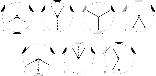
Figure 3: The different types of vertices in the farthest-polygon Voronoi diagram. Pure arcs are shown solid, medial axis arcs dashed. The arrows indicate the direction of increasing $\Phi(x)$ in a neighborhood of the vertex.

Fig. 3 illustrates all different vertex types. Figs. 3(a) and 3(b) show the possible medial axis vertices; they differ in whether the triangle formed by the three features contains the vertex or not. Similarly, Figs. 3(c) and 3(d) show the pure vertex types. The bottom row shows the three possible types of mixed vertices. Again, we have to distinguish whether the three features enclose the vertex or not, and in the latter case we need to distinguish which two features are on the same site.

Consider an arc $\alpha$ of $\mathfrak{F}(\mathcal{S})$. If a point $x$ moves continuously along $\alpha$, then $\Phi(x)$—which is the radius of $D(x)$—changes continuously. The local shape of $\mathfrak{F}(\mathcal{S})$ in a neighborhood of a vertex $v$ is determined solely by the features defining the vertex. For each type of vertex shown in Fig. 3, we can therefore uniquely determine whether $\Phi(x)$ increases or decreases along an arc in a neighborhood of the vertex. We indicate the direction of increasing $\Phi(x)$ along an arc by arrows in the figure.

In addition to the seven types of vertices discussed above, we need to consider vertices at infinity, that is, we consider the semi-infinite arcs of $\mathfrak{F}(\mathcal{S})$ to have a degree-one vertex at their end. For a vertex $v$ at infinity, the “disk” $D(v)$ is a halfplane, and we have two cases:

• If $D(v)$ touches one site $P$ in two features, and all other sites intersect the interior of $D(v)$, then $D(v)$ is the “infinite” endpoint of a medial axis arc, and we consider it a medial axis vertex at infinity.

• If $D(v)$ touches two distinct sites, and all other sites intersect its interior, then $D(v)$ is the “infinite” endpoint of a pure edge, and we consider it a pure vertex at infinity.

Finally, we define the Voronoi region of a site $P\in\mathcal{S}$. The Voronoi region $\mathcal{R}(P)$ of $P$ is simply the union of all cells, medial axis arcs, and medial axis vertices of $\mathfrak{F}(\mathcal{S})$ belonging to features of $P$. Voronoi regions are not necessarily connected, as we will see in the next section. We call each connected component of a Voronoi region a Voronoi component.

3 Structure and complexity

In this section, we prove some properties on the structure of farthest-polygon Voronoi diagrams of polygonal sites and we bound their complexity. Farthest-polygon Voronoi diagrams contain three different types of vertices, as defined in the previous section. Note first that the number of medial axis vertices is bounded by the total complexity of all medial axes, which is $O(n)$.

Now, we first bound the number of mixed vertices. For that purpose, we show that when a tree $\mathcal{T}$ of $\mathfrak{M}(P)$ intersects the Voronoi region $\mathcal{R}(P)$ of $P\in\mathcal{S}$, then the intersection $\mathcal{T}\cap\mathcal{R}(P)$ is a connected subtree. We start with a preliminary lemma.

Lemma 1.

Let $\gamma$ be a path in $\mathfrak{M}(P)$, let $Q\in\mathcal{S}\setminus\{P\}$ be another site, and let $\gamma_{Q}$ be the part of $\gamma$ that is closer to $Q$ than to $P$. Then $\gamma_{Q}$ is a connected subset of $\gamma$, that is, a subpath.

Proof.

We can assume $\gamma$ to be a maximal path in $\mathcal{T}$, connecting a corner $w$ of $P$ with another corner $u$ or a medial-axis vertex at infinity. Assume for a contradiction that there are points $x$, $y$, $z$ on $\gamma$ in this order such that $x,z\in\gamma_{Q}$, but $y\not\in\gamma_{Q}$.

We first consider the case where $y$ lies on a spoke of $\mathfrak{M}(P)$ induced by a corner $c$ of $P$ (and one of its incident edges). The spoke is incident to a leaf of $\mathfrak{M}(P)$ located at $c$ and, without loss of generality, $x$ lies on this spoke between $c$ and $y$. Since $y\not\in\gamma_{Q}$, the disk $D_{P}(y)$ centered at $y$ and touching $c$ does not intersect $Q$. The disk $D_{P}(x)$ is included in $D_{P}(y)$ and thus, it does not intersect $Q$ either, which contradicts our hypothesis.

We now consider the case where $y$ does not lie on a spoke of $\mathfrak{M}(P)$. Let ${\Omega}$ be the connected component of $\mathbb{R}^{2}\setminus P$ that contains $y$. Since $y$ does not lie on a spoke of $\mathfrak{M}(P)$, the disk $D_{P}(y)$ touches $P$ in $k\geqslant 2$ distinct points ($k\leqslant 3$ by the general position assumption), and thus $D_{P}(y)$ partitions ${\Omega}$ into $k+1$ connected components: $D_{P}(y)$ and $k$ other components denoted $A_{1},\ldots,A_{k}$. Since $P$ is a polygon, the structure of its medial axis is well understood. In particular, in the neighborhood of $y$, $\mathfrak{M}(P)$ consists of $k$ arcs (straight or parabolic), and for every point $p$ on any single one of these arcs, $D_{P}(p)$ intersects one and the same components $A_{i}$, and is contained in $A_{i}\cup D_{P}(y)$. Also, since $\mathfrak{M}(P)$ consists of $k$ arcs in the neighborhood of $y$, point $y$ splits the medial axis tree $\mathcal{T}$ that contains $\gamma$ into $k$ subtrees $\mathcal{T}_{1},\ldots,\mathcal{T}_{k}$.

Now, we observe that any open disk $D$, that does not intersect $P$, cannot contain points in two distinct components $A_{i}$ and $A_{j}$. Indeed, the boundary of $D$ would have to intersect the boundary of $D_{P}(y)$ in at least four points, implying that the two disk coincide, and thus that $D$ intersects neither $A_{i}$ nor $A_{j}$ (since $D$ is open).

For any $p\in\mathcal{T}_{i}$, distinct from $y$, $D_{P}(p)$ is included in ${\Omega}$ but not in $D_{P}(y)$. Thus, the interior of $D_{P}(p)$ intersects $\bigcup_{j}A_{j}$ but not $P$. Hence, it intersects only one of the $A_{j}$. Furthermore, by continuity, the interior of $D_{P}(p)$ intersects the same $A_{j}$ for all $p$ in $\mathcal{T}_{i}$. We can thus assume without loss of generality that, for all $p$ in $\mathcal{T}_{i}$, the interior of $D_{P}(p)$ intersects $A_{i}$ and none of the other $A_{j}$. Since $D_{P}(p)$ lies in ${\Omega}$, it also follows that, for all $p$ in $\mathcal{T}_{i}$, $D_{P}(p)$ lies in $A_{i}\cup D_{P}(y)$.

Now, $x$ and $z$ belong to two distinct subtrees, say $\mathcal{T}_{1}$ and $\mathcal{T}_{2}$, respectively. Thus, $D_{P}(x)$ lies in $A_{1}\cup D_{P}(y)$ and $D_{P}(z)$ lies in $A_{2}\cup D_{P}(y)$. By assumption, both $D_{P}(x)$ and $D_{P}(z)$ intersect $Q$, thus $Q$ intersects both $A_{1}\cup D_{P}(y)$ and $A_{2}\cup D_{P}(y)$. Hence, since $Q$ is connected and does not intersect $P$, $Q$ must intersect $D_{P}(y)$, which is a contradiction and concludes the proof. ∎

Lemma 2.

Let $\mathcal{T}$ be a tree of $\mathfrak{M}(P)$. Then $\mathcal{T}\cap\mathcal{R}(P)$ is a connected subtree of $\mathcal{T}$.

Proof.

Pick two points $p,q\in\mathcal{T}\cap\mathcal{R}(P)$, let $\gamma$ be the path on $\mathcal{T}$ from $p$ to $q$, and let $x$ be any point between $p$ and $q$ on $\gamma$. We need to show that $x\in\mathcal{R}(P)$, which is equivalent to showing that $x$ is closer to every site $Q\neq P$ than to $P$. Let $Q$ be such a site. Since $p,q\in\mathcal{R}(P)$, $p$ and $q$ are closer to $Q$ than to $P$. By Lemma 1, this implies that $x$ is closer to $Q$ than to $P$. ∎

The lemma allows us to bound the number of mixed vertices of $\mathfrak{F}(\mathcal{S})$.

Lemma 3.

The number of mixed vertices of $\mathfrak{F}(\mathcal{S})$ for a family of disjoint polygonal sites of total complexity $n$ is $O(n)$.

Proof.

Consider a site $P\in\mathcal{S}$ of complexity $m$. Its medial axis $\mathfrak{M}(P)$ has complexity $O(m)$. By Lemma 2, for each tree $\mathcal{T}$ of $\mathfrak{M}(P)$ the intersection $\mathcal{T}\cap\mathcal{R}(P)$ is a connected subtree. Since the mixed vertices on $\mathcal{T}$ are exactly the finite leaves of this subtree, this implies that the number of mixed vertices on $\mathfrak{M}(P)$ is $O(m)$. Summing over all $P\in\mathcal{S}$ then proves that the number of mixed vertices of $\mathfrak{F}(\mathcal{S})$ is $O(n)$. ∎

We next consider the vertices at infinity.

Lemma 4.

The number of pure vertices at infinity of $\mathfrak{F}(\mathcal{S})$ is at most $2k-2$. The total number of vertices at infinity of $\mathfrak{F}(\mathcal{S})$ is $O(n)$.

Proof.

For two sites $P,Q\in\mathcal{S}$, consider the diagram $\mathfrak{F}(\{P,Q\})$. A pure vertex at infinity corresponds to an edge of $\operatorname{CH}(P\cup Q)$ supported by a corner of $P$ and a corner of $Q$. But $\operatorname{CH}(P\cup Q)$ can have at most two such edges, since $P$ and $Q$ are disjoint and both are connected, and so $\mathfrak{F}(\{P,Q\})$ has at most two pure vertices at infinity.

Consider now again $\mathfrak{F}(\mathcal{S})$, and let $\sigma(\mathcal{S})$ denote the sequence of sites whose Voronoi regions appear at infinity in circular order, starting and ending at the same region. We claim that $\sigma(\mathcal{S})$ is a Davenport-Schinzel sequence of order 2, and has therefore length at most $2k-1$ [19]. Indeed, $\sigma(\mathcal{S})$ has by definition no two consecutive identical symbols. Assume now that there are two sites $P$ and $Q$ such that the subsequence $PQPQ$ appears in $\sigma(\mathcal{S})$. If we delete all other sites, then $\sigma(\{P,Q\})$ would still need to contain the subsequence $PQPQ$, and therefore $\mathfrak{F}(\{P,Q\})$ would contain at least three pure vertices at infinity, a contradiction to the observation above.

It now suffices to observe that the pure vertices at infinity are exactly the transitions between consecutive Voronoi regions, and their number is at most $2k-2$.

All remaining vertices at infinity are medial axis vertices. Since the total complexity of all medial axes is $O(n)$, the bound follows ∎

We proved so far that the number of mixed and medial axis vertices is $O(n)$ and, furthermore, that there are at most $2k-2$ pure vertices at infinity. It remains to bound the other pure vertices, for which we first need to prove a few basic properties.

We start by discussing a monotonicity property of cells of $\mathfrak{F}(\mathcal{S})$. Let $C$ be a cell of $\mathfrak{F}(\mathcal{S})$ belonging to feature $w$ of site $P$. For a point $x\in C$, let $x^{\ast}$ be the point on $w$ closest to $x$. Let $f_{x}$ be the directed line segment starting at $x$ and extending in direction $\overrightarrow{x^{\ast}x}$ until it reaches $\mathfrak{M}(P)$ (a semi-infinite segment if this does not happen). We call $f_{x}$ the fiber of $x$. We note that if $w$ is an edge, then all fibers of $C$ are parallel, and normal to $w$; if $w$ is a corner then all fibers are supported by lines through $w$.

Lemma 5.

For any $x\in C$, the fiber $f_{x}$ lies entirely in $C$ (and therefore in $\mathcal{R}(P)$).

Proof.

The disk $D(x)$ touches $P$ in $x^{\ast}$ only, and its interior intersects all other sites. When we move a point $y$ from $x$ along $f_{x}$, the disk $D$ centered at $y$ through $x^{\ast}$ keeps containing $D(x)$, and it therefore still intersects all other sites. This implies that $y\in C$ as long as $D$ does not intersect $P$ in another point. This does not happen until we reach $\mathfrak{M}(P)$. ∎

An immediate consequence, which we will use for computing Voronoi diagrams (Section 4), is that cells are “monotone”:

Lemma 6.

The boundary of a cell $C$ of $\mathfrak{F}(\mathcal{S})$ belonging to feature $w$ consists of two chains monotone with respect to $w$, that is, monotone in the direction of $w$ if $w$ is an edge, and rotationally monotone around $w$ if $w$ is a corner. The lower chain is closer to the feature and consists of pure arcs only, the upper chain consists of medial axis arcs only.

Proof.

Let $P$ be the site containing the feature $w$. Consider a half-line $\ell$ with origin on $w$, and normal to $w$ if $w$ is an edge. Let $x$ be the point closest to $w$ in $\ell\cap C$. It is straightforward that the entire fiber $f_{x}$ lies in $C$, and no point $z$ on $\ell$ beyond the medial axis can be in $C$ since the feature of $P$ closest to any such $z$ cannot be $w$. Hence, the boundary of $C$ consists of two monotone chains with respect to $w$. Moreover, the upper chain consists of medial axis arcs by definition of the fibers $f_{x}$. The lower chain consists of pure arcs, because if a point $x$ on the lower chain was on the medial axis, then the fiber $f_{x}$ would be reduced to point $x$, by definition; thus $x$ would also be on the upper chain, implying that $x$ is an endpoint of the two chains. ∎

We now show (Lemma 8) that if a Voronoi region is bounded, then it is connected (we actually show that it is simply connected, but will not use that fact in this paper). This property is tight in the sense that, as shown in Lemma 10, a single Voronoi region may consist of up to $k-1$ unbounded connected components; we postpone the proof of this property to the end of the section.

Lemma 7.

If a connected component of the Voronoi region $\mathcal{R}(P)$ of a site $P\in\mathcal{S}$ is bounded, then $P$ properly contains another site inside one of its pockets.

Proof.

Let $C$ be a bounded connected component of $\mathcal{R}(P)$. We first observe that $C$ contains some points of the medial axis $\mathfrak{M}(P)$ of $P$. Indeed, let $x\in C$ and consider its fiber $f_{x}$. By Lemma 5 and since $C$ is bounded, $f_{x}$ does not extend to infinity and, therefore, one of its endpoints lies on $\mathfrak{M}(P)$.

Let $x$ be a point in $C\cap\mathfrak{M}(P)$. If $x$ lies in a pocket of $P$ that does not share an edge with $\operatorname{CH}(P)$ (that is, the pocket is a hole in $P$), then this pocket does contain all the other sites in $\mathcal{S}\setminus\{P\}$ and the lemma is proven. Otherwise, we let $x$ move along the medial axis $\mathfrak{M}(P)$ up to infinity. At some point $x^{\prime}$, the point must exit from the bounded region $C$. This means that $D_{\mathcal{S}}(x^{\prime})=D_{P}(x^{\prime})$ is tangent to another site $Q$ and does no longer intersect it properly. It then follows from the fact that $x^{\prime}$ lies on the medial axis of $P$ that the site $Q$ lies entirely in the pocket of $P$ associated with the tree of $\mathfrak{M}(P)$ containing $x$ and $x^{\prime}$. ∎

Lemma 8.

If a connected component of the Voronoi region $\mathcal{R}(P)$ of a site $P\in\mathcal{S}$ is bounded, then $\mathcal{R}(P)$ is simply connected.

Proof.

By Lemma 7, $P$ contains another site $Q$ in one of its pockets $\mathfrak{P}$. Let $\mathcal{T}$ be the tree of $\mathfrak{M}(P)$ that corresponds to $\mathfrak{P}$.

Let $x$ be any point in $\mathcal{R}(P)$. The disk $D(x)$ touches $P$ in a point $x^{\ast}$, and its interior intersects all other sites, including $Q$. Hence, $D(x)$ properly intersects the pocket $\mathfrak{P}$. It follows that when moving a point $y$ from $x$ in the direction of $\overrightarrow{x^{\ast}x}$, the disk centered at $y$ through $x^{\ast}$ keeps containing $D(x)$, and it therefore keeps intersecting $\mathfrak{P}$. This implies that, at some finite point $y=x^{\prime}$, the disk $D$ centered at $x^{\prime}$ and tangent to $P$ at $x^{\ast}$ becomes tangent to $P$ at some other point, hence $x^{\prime}$ lies on $\mathfrak{M}(P)$. Moreover, $x^{\prime}$ lies on the tree $\mathcal{T}$ because the disk $D$ properly intersects $\mathfrak{P}$.

Hence, for any point $x$ in $\mathcal{R}(P)$, the fiber $f_{x}$ is a segment joining $x$ to a point $x^{\prime}$ on $\mathcal{T}$. Furthermore, the fiber $f_{x}$ lies in $\mathcal{R}(P)$, by Lemma 5, and $\mathcal{T}\cap\mathcal{R}(P)$ is a connected tree, by Lemma 2. Therefore, $\mathcal{R}(P)$ is connected.

It remains to show that $\mathcal{R}(P)$ is simply connected. We have shown that for any $x\in\mathcal{R}(P)$, the fiber $f_{x}$ is a segment contained in $\mathcal{R}(P)$, and connecting $x$ to $x^{\prime}\in\mathcal{T}\cap\mathcal{R}(P)$. By moving the points of $\mathcal{R}(P)$ along their fiber, we can design, as follows, a continuous deformation retraction of $\mathcal{R}(P)$ onto the tree $\mathcal{T}\cap\mathcal{R}(P)$ which implies that $\mathcal{R}(P)$ is simply connected.

More precisely, it easy to check that the map $F:\mathcal{R}(P)\times[0,1]\rightarrow\mathbb{R}^{2}$, $(x,t)\mapsto(1-t)\,x+t\,x^{\prime}$ is continuous. Furthermore, $F$ is a (strong) deformation retraction since, for all $x\in\mathcal{R}(P)$, $t\in[0,1]$ and $m\in\mathcal{T}\cap\mathcal{R}(P)$, we have $F(x,0)=x$, $F(x,1)\in\mathcal{T}\cap\mathcal{R}(P)$, and $F(m,t)=m$. We have thus exhibited a deformation retraction of $\mathcal{R}(P)$ onto $\mathcal{T}\cap\mathcal{R}(P)$, which implies that these two point sets have the same fundamental group [10, Proposition 1.17]. Since $\mathcal{T}\cap\mathcal{R}(P)$ is a tree, its fundamental group is trivial and so is the fundamental group of $\mathcal{R}(P)$. Any pair of points $x$ and $y$ in $\mathcal{R}(P)$ can be connected with a path made of their fibers $f_{x}$ and $f_{y}$ and a path in $\mathcal{T}\cap\mathcal{R}(P)$, thus $\mathcal{R}(P)$ is path connected. Together with having a trivial fundamental group, this property makes $\mathcal{R}(P)$ simply connected [10, p. 28]. ∎

We can now conclude our analysis of the complexity of farthest-polygon Voronoi diagrams.

Theorem 9.

The farthest-polygon Voronoi diagram of a family of $k$ disjoint polygonal sites of total complexity $n$ has $O(k)$ pure vertices and total complexity $O(n)$. It consists of at most $2k-2$ Voronoi components and this bound is tight in the worst case.

Proof.

The farthest-polygon Voronoi diagram contains three different kinds of vertices. The number of medial axis vertices is clearly only $O(n)$, since the total complexity of all $\mathfrak{M}(P)$ for $P\in\mathcal{S}$ is only $O(n)$. In Lemma 3, we showed that the number of mixed vertices is also only $O(n)$. It remains to bound the number of pure vertices of $\mathfrak{F}(\mathcal{S})$.

Let $k_{1}$ be the number of bounded Voronoi components. By Lemma 8, each of these components corresponds to a different site and only the remaining $k-k_{1}$ sites can contribute to form vertices at infinity. By the proof of Lemma 4, there are at most $2(k-k_{1})-2$ pure vertices at infinity, and therefore at most $2(k-k_{1})-2$ unbounded Voronoi components. It follows that the total number of Voronoi components is at most $2k-k_{1}-2\leqslant 2k-2$. Moreover, the construction of Lemma 10 shows that this bound is tight.

Let us now consider the graph $G$ formed by the pure arcs and pure vertices of $\mathfrak{F}(\mathcal{S})$. Mixed vertices appear as vertices of degree two in $G$ (see Fig. 3), medial axis vertices do not appear at all. The faces of $G$ are exactly the Voronoi components. Since $G$ has at most $2k-2$ faces, Euler’s formula implies that $G$ has $O(k)$ vertices of degree three. ∎

Finally, we prove that, as mentioned above, a single Voronoi region of $\mathfrak{F}(\mathcal{S})$ can have up to $k-1$ connected components.

Figure 4: The Voronoi region of polygon $R$ has $k-1$ connected components.

Lemma 10.

A single Voronoi region of $\mathfrak{F}(\mathcal{S})$ can have $k-1$ connected components and this bound is tight.

Proof.

The construction is shown in Fig. 4. It consists of one $(k-1)$-regular polygon $R$ and $k-1$ polygonal chains $C_{1},\ldots,C_{k-1}$. Let $e_{1},e_{2},\ldots,e_{k-1}$ denote the edges of $R$ in circular order. We inductively construct the polygonal sites $C_{i},i=1,2,\ldots,k-1$ as follows. For the supporting line $l$ of $e_{i}$, let $l^{+}$ be the closed halfplane containing $R$ and $l^{-}$ be the other. Then, consider the intersection $C_{i}^{*}$ between $l^{+}$ and the four edges of a square that contains $R,C_{1},\ldots,C_{i-1}$ inside. We define $C_{i}$ as the set of points of $C_{i}^{*}$ whose distance to $l$ is larger than some fixed small $\varepsilon>0$. $C_{i}$ has at most four edges. Note that $l^{+}$ contains $C_{i}$ completely. Consider a ray from $e_{i}$ to infinity in $l^{-}$ which is orthogonal to $l$. Since $l^{-}$ intersects all sites but $C_{i}$, the endpoint at infinity of this ray lies in the region $\mathcal{C}_{i}=\mathcal{R}(C_{i})$. On the other hand, for a sufficiently small $\varepsilon$, there is a line $L$ passing through $v_{i}$ (the vertex incident to $e_{i-1}$ and $e_{i}$) such that we can define $L^{+}$ as an open halfplane containing $R\backslash\{v_{i}\}$ and $L^{-}$ as the other open halfplane intersecting all the other sites but $R$. The endpoint at infinity of the ray from $v_{i}$ to infinity in $L^{-}$ which is orthogonal to $L$ lies in a connected component of $\mathcal{R}(R)$, which we call $\mathcal{R}_{i}$.

Therefore at infinity $\mathcal{R}_{1},\mathcal{C}_{1},\mathcal{R}_{2},\mathcal{C}_{2},\cdots,\mathcal{R}_{k-1},\mathcal{C}_{k-1}$ appear in turn. Note that for a point $x$ in the region $\mathcal{R}(R)$, its fiber $f_{x}$ is an infinite ray because $R$ is convex. For $i=1,2,\ldots,k-1$, consider the half-line $x_{i}\phi_{i}$ from a point at infinity $\phi_{i}\in\mathcal{C}_{i}$ to a point $x_{i}\in R$ closest to $\phi_{i}$. If $x\in x_{i}\phi_{i}$ lies in $\mathcal{R}(R)$, then $f_{x}\subset\mathcal{R}(R)$, which is impossible because $\phi_{i}\in\mathcal{C}_{i}$. Define $W=R\cup\bigcup_{i}{x_{i}\phi_{i}}$. We then have $W\cap\mathcal{R}(R)=\emptyset$, and $\mathbb{R}^{2}\setminus W$ consists of $k-1$ unbounded connected subsets of the plane. The connected subset bounded by $x_{i}\phi_{i}$, $x_{i+1}\phi_{i+1}$ and $R$ contains $\mathcal{R}_{i}$ completely. It follows that $\mathcal{R}_{i}\neq\mathcal{R}_{j}$ when $i\neq j$.

It remains to show that the bound of $k-1$ is tight. By Lemma 4, there are at most $2k-2$ pure vertices at infinity, and thus at most $2k-2$ unbounded Voronoi components. Hence, one single Voronoi region has at most $k-1$ unbounded Voronoi components (since two neighboring components cannot correspond to the same site). This concludes the proof because, by Lemma 8, if a Voronoi region has a bounded component, then the entire region is connected. ∎

4 Algorithm

The proof of Theorem 9 suggests an algorithm for computing the Voronoi diagram by sweeping the arcs of the graph $G$. This is roughly equivalent to computing the surface $\Phi$ by sweeping a horizontal plane downwards, and maintaining the part of $\Phi$ above this plane. This is essentially the approach used by Aurenhammer et al. [3] for the computation of farthest-segment Voronoi diagrams. However, this does not seem to work for our diagram because of the mixed vertices of type (f) (see Fig. 3), where $\Phi$ has a local maximum. We instead offer a divide-and-conquer algorithm.

Theorem 11.

The farthest-polygon Voronoi diagram $\mathfrak{F}(\mathcal{S})$ of a family $\mathcal{S}$ of disjoint polygonal sites of total complexity $n$ can be computed in time $O(n\log^{3}n)$.

Proof.

Let $\mathcal{S}=\{P_{1},\dots,P_{k}\}$, and let $n_{i}$ be the complexity of $P_{i}$. If $k=1$, then $\mathfrak{F}(\mathcal{S})$ is simply the medial axis $\mathfrak{M}(P_{1})$, which can be computed in time $O(n\log n)$ [9]. Otherwise, we split $\mathcal{S}$ into two disjoint families $\mathcal{S}_{1},\mathcal{S}_{2}$ as follows:

• If there is a site $P_{i}$ with complexity $n_{i}\geqslant n/2$, then $\mathcal{S}_{1}=\{P_{i}\}$ and $\mathcal{S}_{2}=\mathcal{S}\setminus\{P_{i}\}$.

• Otherwise there must be an index $j$ such that $n/4\leqslant\sum_{i=1}^{j}n_{i}\leqslant 3n/4$. We let $\mathcal{S}_{1}=\{P_{1},\dots,P_{j}\}$ and $\mathcal{S}_{2}=\{P_{j+1},\dots,P_{k}\}$.

We recursively compute $\mathfrak{F}(\mathcal{S}_{1})$ and $\mathfrak{F}(\mathcal{S}_{2})$. We show in the rest of this section (see Lemma 17) that we can then merge these two diagrams to obtain $\mathfrak{F}(\mathcal{S})$ in time $O(n\log^{2}n)$, proving the theorem. ∎

We now discuss the merging step. We are given the farthest-polygon Voronoi diagrams $\mathfrak{F}(\mathcal{S}_{1})$ and $\mathfrak{F}(\mathcal{S}_{2})$ of two families $\mathcal{S}_{1}$ and $\mathcal{S}_{2}$ of pairwise disjoint polygonal sites, and let $\mathcal{S}=\mathcal{S}_{1}\cup\mathcal{S}_{2}$.

Consider the diagram $\mathfrak{F}(\mathcal{S})$ to be computed. We color the Voronoi regions of $\mathfrak{F}(\mathcal{S})$ defined by sites in $\mathcal{S}_{1}$ red, and the Voronoi regions defined by sites in $\mathcal{S}_{2}$ blue. A pure arc of $\mathfrak{F}(\mathcal{S})$ is red if it separates two red regions, and blue if it separates two blue regions. The remaining pure arcs, which separate a red and a blue region, are called purple. A vertex of $\mathfrak{F}(\mathcal{S})$ is purple if it is incident to a purple arc. We observe (see Fig. 3) that, by our general position assumption, every purple vertex not at infinity is incident to exactly two purple arcs, and so the purple arcs form a collection of bounded and unbounded chains (see Fig. 5).

As we will see in Lemma 17, merging $\mathfrak{F}(\mathcal{S}_{1})$ and $\mathfrak{F}(\mathcal{S}_{2})$ can be done in linear time once all purple arcs are known, because the diagram $\mathfrak{F}(\mathcal{S})$ consists of those portions of $\mathfrak{F}(\mathcal{S}_{1})$ lying in the red regions of $\mathfrak{F}(\mathcal{S})$, and those portions of $\mathfrak{F}(\mathcal{S}_{2})$ lying in the blue regions of $\mathfrak{F}(\mathcal{S})$, see Fig. 5.

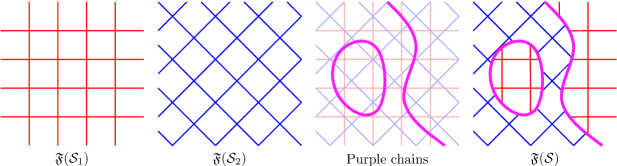
Figure 5: Merging $\mathfrak{F}(\mathcal{S}_{1})$ and $\mathfrak{F}(\mathcal{S}_{2})$ to obtain $\mathfrak{F}(\mathcal{S})$.

We show below how the purple chains of $\mathfrak{F}(\mathcal{S})$ can be computed in time $O(n\log^{2}n)$. We first show how to compute at least one point on every chain and then how to “trace” a chain from a starting point.

Lemma 12.

The vertices at infinity of the purple chains can be computed in time $O(n\log n)$.

Proof.

We show how to compute all the pure vertices at infinity in time $O(n\log n)$. There are $O(k)$ such pure vertices (by Lemma 4), and we can easily deduce the purple ones from those in $O(k)$ time.

For site $P_{i}\in\mathcal{S}$ and angle $\phi\in[0,2\pi)$, let $\ell_{i}(\phi)$ be the oriented line with direction $\phi$ tangent to $P_{i}$ and keeping $P_{i}$ entirely on its left, see Fig. 6. Let $g_{i}(\phi)$ be the signed distance from the origin to $\ell_{i}(\phi)$ (positive if the origin lies left of $\ell_{i}(\phi)$, negative otherwise). If $P_{i}$ is a polygonal site of complexity $m$, we first compute the convex hull $\operatorname{CH}(P_{i})$ in time $O(m\log m)$, and we deduce a description of the function $g_{i}$ in time $O(m)$.

We then compute the lower envelope $g$ of the functions $g_{i}$. The pure vertices at infinity correspond exactly to the breakpoints of this lower envelope, since they correspond to half-planes (or disks with centers at infinity) touching two sites and whose interiors intersect all other sites. Such a half-plane is illustrated in gray in Fig. 6. Moreover, two functions $g_{i}$, $g_{j}$ can intersect at most twice since each intersection corresponds to a pure vertex at infinity of $\mathfrak{F}(\{P_{i},P_{j}\})$ which admits at most two such vertex as argued in the proof of Lemma 4. Hence, the lower envelope can be computed in time $O(n\log n)$ [19]. ∎

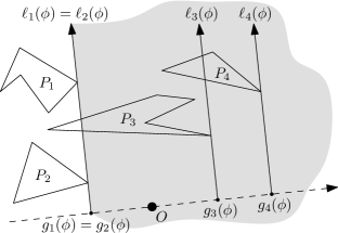
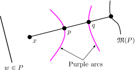
Figure 6: (a) Constructing the pure vertices at infinity. (b) For the proof of Lemma 15: a fiber $f_{x}$ cannot have more than one intersection point with purple arcs.

Lemma 13.

Any bounded purple chain contains a mixed vertex of $\mathfrak{F}(\mathcal{S})$.

Proof.

A bounded purple chain is a compact set in the plane, and so the restriction of $\Phi(\cdot)$ to such a chain admits a maximum. Such a maximum appears at a vertex, denoted $v$. Indeed, since an arc $\alpha$ of $\mathfrak{F}(\mathcal{S})$ is defined by two features (corners or edges), the graph of $\Phi(\cdot)$ restricted to $\alpha$ is the intersection of the two Voronoi surfaces—which are cones or wedges—induced by the two features; thus $\Phi(\cdot)$ cannot have a local maximum in the interior of $\alpha$ (it may have a local minimum).

Consider now the arcs of $\mathfrak{F}(\mathcal{S})$ oriented, in a neighborhood of their endpoints, in the direction of increasing $\Phi(\cdot)$. Then, the two purple arcs incident to $v$ point toward $v$. Now observe that purple arcs are pure and a vertex incident to at least two pure arcs pointing toward it is of type (e) or (f), which is mixed (see Fig. 3). Hence, $v$ is a mixed vertex of $\mathfrak{F}(\mathcal{S})$, which concludes the proof. ∎

Lemma 14.

Given the farthest-polygon Voronoi diagrams of two families $\mathcal{S}_{1}$ and $\mathcal{S}_{2}$ of pairwise disjoint polygonal sites, the mixed vertices of $\mathfrak{F}(\mathcal{S}_{1}\cup\mathcal{S}_{2})$ can be computed in time $O(n\log^{2}n)$.

Computing the mixed vertices in time $O(n\log^{2}n)$ is the most subtle part of the algorithm and we postpone the proof of this lemma to Section 4.1, after showing how to compute the purple chains from some starting point (Lemma 16). We start with a preliminary lemma which is an important consequence of Lemma 5.

Lemma 15.

Let $f_{x}$ be the fiber of point $x$ in a cell $C$ of $\mathfrak{F}(\mathcal{S}_{1})$ or $\mathfrak{F}(\mathcal{S}_{2})$. Then, the relative interior of $f_{x}$ intersects the purple arcs of $\mathfrak{F}(\mathcal{S})$ in at most one point.

Proof.

Assume, for a contradiction, that the relative interior of $f_{x}$ intersects two purple arcs in two distinct points $p$ and $q$, where $q$ lies on $f_{p}$ (see Fig. 6). We can assume, without loss of generality that the purple chain and $f_{x}$ cross at $p$, because, otherwise, there exists another fiber close to $f_{x}$ (for instance, $f_{y}$ for some $y$ close to $x$) that intersects transversally the purple chains in two points. Now, let $P$ be the site containing the feature $w$ associated with $C$. In $C$, the purple arcs bound the cell of $\mathfrak{F}(\mathcal{S})$ belonging to feature $w$. Hence, there is a point $p^{\prime}$ on $f_{x}$ sufficiently close to $p$ such that $p^{\prime}\in\mathcal{R}(P)$ in $\mathfrak{F}(\mathcal{S})$. Moreover, the fiber $f_{p^{\prime}}$ is, by definition, a subset of the fiber $f_{x}$. Thus, the fiber $f_{p^{\prime}}$ contains $q$ and thus intersects a purple arc, contradicting the fact that $f_{p^{\prime}}$ lies in $\mathcal{R}(P)$ in $\mathfrak{F}(\mathcal{S})$ (by Lemma 5). ∎

Lemma 16.

Given the farthest-polygon Voronoi diagrams $\mathfrak{F}(\mathcal{S}_{1})$ and $\mathfrak{F}(\mathcal{S}_{2})$ of two families $\mathcal{S}_{1}$ and $\mathcal{S}_{2}$ of pairwise disjoint polygonal sites, the purple chains of $\mathfrak{F}(\mathcal{S}_{1}\cup\mathcal{S}_{2})$ can be computed in time $O(n\log^{2}n)$.

Proof.

By Lemmas 12, 13 and 14, we can compute the vertices at infinity of the purple chains, and a superset of size $O(n)$ of at least one mixed vertex per bounded component. As we have seen in the proof of Lemma 13, these latter vertices are of type (e) or (f) (see Fig. 3); they thus involve only two sites and we discard all those that involve two sites of $\mathcal{S}_{1}$ or two sites of $\mathcal{S}_{2}$. We thus obtain a set of $O(n)$ purple vertices with at least one such vertex on each purple chain. We consider each such vertex, denoted $v$, in turn, and “trace” (construct) the purple chain that $v$ lies on.

If $v$ is at infinity, there is only one purple arc incident to it; otherwise, there are two and we consider one of them. The bisector supporting the incident purple arc is that of one red and one blue feature among the features defining $v$. Splitting the bisector at $v$ defines two semi-infinite curves incident to $v$ and we can determine, using the respective position of the three features defining $v$, which of these two curves supports the considered purple arc; we call this semi-infinite curve a purple half-bisector.

We then trace the purple chain by following its purple arcs from cell to cell: observe that the other endpoint of the considered purple arc incident to $v$ is either at infinity or is the first intersection point (starting from $v$) between the purple half-bisector and the cell boundaries of $\mathfrak{F}(\mathcal{S}_{1})$ and $\mathfrak{F}(\mathcal{S}_{2})$. We compute this point as follows.

We first locate $v$ in $\mathfrak{F}(\mathcal{S}_{1})$ and $\mathfrak{F}(\mathcal{S}_{2})$. This can be done in $O(\log n)$ time, assuming that we have precomputed a point-location data structure for $\mathfrak{F}(\mathcal{S}_{1})$ and $\mathfrak{F}(\mathcal{S}_{2})$ in $O(n\log n)$ time (see, for instance, [8]).  Note that $v$ is a vertex of $\mathfrak{F}(\mathcal{S})$ and that it involves two features of one site, say in $\mathcal{S}_{1}$, thus $v$ lies on a medial axis arc of $\mathfrak{F}(\mathcal{S}_{1})$ induced by these two features. We then also determine the cell of $\mathfrak{F}(\mathcal{S}_{1})$, denoted $C_{1}$, that contains the purple half-bisector in a neighborhood of $v$ (this is a constant size problem). Since $v$ is a purple vertex, its third feature belongs to a site of $\mathcal{S}_{2}$, and $v$ lies in the cell of $\mathfrak{F}(\mathcal{S}_{2})$, denoted $C_{2}$, belonging to that feature. Let $w_{i}$ denote the feature associated with $C_{i}$, $i=1,2$.

Then, for $i=1,2$, we sweep the cell $C_{i}$ with a line orthogonal to the feature $w_{i}$ if $w_{i}$ is an edge and with a line through the feature $w_{i}$ if $w_{i}$ is a corner. If $w_{i}$ is a corner, the sweep is done clockwise or counterclockwise so that the sweep line intersects the half-bisector inside $C_{i}$ (deciding between clockwise or counterclockwise is a constant size problem); the situation is similar when $w_{i}$ is an edge.

The two cells $C_{1}$ and $C_{2}$ are swept simultaneously. However, since the two sweeps are not a priori performed using the same sweep line, this requires some care. For clarity, we first present each sweep independently.

By Lemma 6, the sweep line always intersects one arc of the upper chain of $C_{i}$ (or two arcs at their common endpoints) and similarly for the lower chain. We first determine the arcs of the upper and lower chains that are intersected by the sweep line through $v$ (or about to be intersected if the sweep line goes through a vertex of the chain). We also determine the intersection, if any, of these two arcs with the purple half-bisector. When the sweep line reaches an endpoint of one of the two arcs that are being swept, we determine the intersection (if any) between the new arc and the purple half-bisector. When the sweep line reaches the first of the computed intersection points between the purple half-bisector and the boundary of the cell, we report this intersection point and terminate the sweep of $C_{i}$.

If the two sweeps were performed independently, we could report the first point where the purple half-bisector exits one of the cells $C_{1}$ or $C_{2}$, and continues the tracing in a neighboring cell of either $\mathfrak{F}(\mathcal{S}_{1})$ or $\mathfrak{F}(\mathcal{S}_{2})$, along a new purple half-bisector. This however would not yield the claimed complexity because, roughly speaking, if a sequence of purple arcs enter and exit $\Theta(n)$ cells $C_{1},C_{1}^{\prime},C_{1}^{\prime\prime},\ldots$ while remaining inside a cell $C_{2}$ of complexity $\Theta(n)$, the cell $C_{2}$ would be swept many times, possibly leading to a complexity of $\Theta(n\log n)$ per arc, and a total of $\Theta(n^{2}\log n)$. We thus perform the two sweeps simultaneously, as follows.

Note first that, by Lemma 15, during the sweep of $C_{i}$, the point of intersection, in $C_{i}$, between the sweep line and the purple half-bisector moves monotonically along the purple half-bisector. We can thus parameterize the sweeps of $C_{1}$ and $C_{2}$ by a point $x$ moving monotonically on the purple half-bisector away from $v$. The point $x$ define two sweep lines (the lines through $x$ and through $w_{i}$ or orthogonal to $w_{i}$ depending on the nature of $w_{i}$), and the events are those of the sweeps of $C_{1}$ and $C_{2}$. This sweep ends when the purple half-bisector leaves $C_{1}$ or $C_{2}$. Then, the tracing of the purple chain continues in a neighboring cell of either $\mathfrak{F}(\mathcal{S}_{1})$ or $\mathfrak{F}(\mathcal{S}_{2})$, along a new purple half-bisector. We stop tracing the purple chain when we reach a vertex at infinity or the vertex $v$ we started from.

We then consider a new starting point $v$; note that we can easily check in $O(\log n)$ time whether it has already been computed (while tracing some purple chains) by maintaining the list of the already computed vertices on the purple chains, ordered lexicographically by their features.

We now analyze the complexity of the algorithm. Consider first the initialization of every sweep, that is the determination of the arcs of $C_{1}$ and $C_{2}$ that are intersected by the two sweep lines through $v$. There are $O(n)$ such initialization steps to perform, since $\mathfrak{F}(\mathcal{S})$ have size $O(n)$ by Theorem 9, and each step can be done using binary search in $O(\log n)$ time, after preprocessing all the cells of $\mathfrak{F}(\mathcal{S}_{1})$ and $\mathfrak{F}(\mathcal{S}_{2})$; the preprocessing (which simply is storing the ordered vertices of the upper and lower chains of each cell in arrays) can be done in time linear in the total size of the cells, which is $O(n)$, by Theorem 9.

We finally analyze the complexity of the rest of the algorithm by applying a simple charging scheme. Note first that intersecting the purple half-bisector with an arc of a cell takes constant time. We charge the cost of computing these intersections to either the purple vertices or to the arcs of $C_{i}$, as follows. The intersections with each of the arcs that are swept at the beginning and the end of the sweep are charged to the corresponding endpoint of the purple arc. Every purple vertex is thus charged at most eight times because each of the two incident purple edges is intersected with one arc of each of the lower and upper chains of each of the two cells $C_{1}$ and $C_{2}$. The intersections with each of the other arcs of $C_{i}$ are charged to the arc in question. Every such arc is charged at most once per cell, and thus at most twice in total; indeed, such an arc of $C_{i}$ is swept entirely during the sweep of $C_{i}$ and thus, by Lemma 15, it will not be swept again during another sweep of cell $C_{i}$ (when treating another purple half-bisector). Since $\mathfrak{F}(\mathcal{S}_{1})$, $\mathfrak{F}(\mathcal{S}_{2})$, and $\mathfrak{F}(\mathcal{S})$ have size $O(n)$ (Theorem 9), all the purple arcs can be computed in $O(n\log n)$ time, in total, once the set of starting points are known, and thus in $O(n\log^{2}n)$ time by Lemmas 12 and 14. ∎

Lemma 17.

Given the farthest-polygon Voronoi diagrams of two families $\mathcal{S}_{1}$ and $\mathcal{S}_{2}$ of pairwise disjoint polygonal sites, the farthest-polygon Voronoi diagrams of $\mathcal{S}_{1}\cup\mathcal{S}_{2}$ can be computed in time $O(n\log^{2}n)$.

Proof.

During the computation of the purple chains (see the proof of Lemma 16), we can split the arcs of $\mathfrak{F}(\mathcal{S}_{1})$ and $\mathfrak{F}(\mathcal{S}_{2})$ at every new purple vertex that is computed. Then, merging $\mathfrak{F}(\mathcal{S}_{1})$ and $\mathfrak{F}(\mathcal{S}_{2})$ can trivially be done in linear time since, as we mentioned before, the diagram $\mathfrak{F}(\mathcal{S})$ consists of those portions of $\mathfrak{F}(\mathcal{S}_{1})$ lying in the red regions of $\mathfrak{F}(\mathcal{S})$, and those portions of $\mathfrak{F}(\mathcal{S}_{2})$ lying in the blue regions of $\mathfrak{F}(\mathcal{S})$, see Fig. 5. ∎

4.1 Computing the mixed vertices

We prove here Lemma 14 stating that, given the farthest-polygon Voronoi diagrams of two families $\mathcal{S}_{1}$ and $\mathcal{S}_{2}$ of pairwise disjoint polygonal sites, the mixed vertices of $\mathfrak{F}(\mathcal{S}_{1}\cup\mathcal{S}_{2})$ can be computed in time $O(n\log^{2}n)$.

We start by computing the randomized point-location data structure of Mulmuley [17] (see also [6, Chapter 6]) for the two given Voronoi diagrams $\mathfrak{F}(\mathcal{S}_{1})$ and $\mathfrak{F}(\mathcal{S}_{2})$. (We chose this randomized algorithm for its simplicity; randomization can however be avoided as we explain at the end of this section.) This data structure only needs two primitive operations: (i) for a given point $p$ in the plane, determine whether the query point lies left or right of $p$, and (ii) for an $x$-monotone line segment or parabolic arc $\gamma$, determine whether the query point lies above or below $\gamma$. Both cases can be summarized as follows: Given a comparator $\gamma$, determine on which side of $\gamma$ the query point lies. The comparator can be either a line or a parabolic arc.

We compute the mixed vertices lying on each tree $\mathcal{T}$ of each medial axis $\mathfrak{M}(P)$ separately. The intersection $\mathcal{T}\cap\mathcal{R}(P)$ is a connected subtree by Lemma 2. We can locate the internal vertices of this subtree easily, by performing a point location operation for each vertex $v$ of $\mathcal{T}$ in $\mathfrak{F}(\mathcal{S}_{1})$ and $\mathfrak{F}(\mathcal{S}_{2})$, deducing which site is farthest from $v$ and checking if the farthest site from $v$ is $P$. Let $I$ be the set of vertices of $\mathcal{T}$ that lie in $\mathcal{R}(P)$. We now need to consider two cases.

4.1.1 When $I$ is not empty

If $I$ is non-empty, then every arc $\alpha$ of $\mathcal{T}$ incident to one vertex in $I$ and one vertex not in $I$ must contain exactly one mixed vertex $s^{\ast}$ by Lemma 2. To locate this vertex $s^{\ast}$, we use parametric search along the arc $\alpha$ [14], albeit in a restricted way, as we do not need to use parallel computation: The idea is to execute two point location queries in $\mathfrak{F}(\mathcal{S}_{1})$ and $\mathfrak{F}(\mathcal{S}_{2})$ using $s^{\ast}$ as the query point. Each query executes a sequence of primitive operations, where we compare the (unknown) location of $s^{\ast}$ with a comparator $\gamma$ (a line or a parabolic arc). This primitive operation can be implemented by intersecting $\alpha$ with $\gamma$, resulting in a set of at most four points. In $O(\log n)$ time, we can test for each of these points whether it lies in $\mathcal{R}(P)$. This tells us between which of these points the unknown mixed vertex $s^{\ast}$ lies, and we can answer the primitive operation.

It follows that we can execute the two point location queries on $s^{\ast}$ in time $O(\log^{2}n)$, and we obtain one cell and one arc of $\mathfrak{F}(\mathcal{S}_{1})$ and $\mathfrak{F}(\mathcal{S}_{2})$ containing $s^{\ast}$ (for instance if $P\in\mathcal{S}_{1}$ then $s^{\ast}$ lies on an arc of $\mathfrak{F}(\mathcal{S}_{1})$ and in a cell of $\mathfrak{F}(\mathcal{S}_{2})$). The mixed vertex $s^{\ast}$ lies at equal distance of the three features to which the arc and cell belong (two of which are features of $P$).

4.1.2 When $I$ is empty

It remains to consider the case where $I$ is empty, that is, no vertex of $\mathcal{T}$ lies in $\mathcal{R}(P)$. Nevertheless, the region $\mathcal{R}(P)$ may intersect a single arc $\alpha$ of $\mathcal{T}$. In this case, Lemma 2 tells us that there are two mixed vertices on $\alpha$ that we need to find. We first need to identify the arcs of $\mathcal{T}$ where this could happen.

Let $p$ and $q$ be two points on the same arc $\alpha$ of $\mathfrak{M}(P)$. We define the cylinder $\mathfrak{C}(p,q)$ of the pair $(p,q)$ as

$$\mathfrak{C}(p,q)=\bigcup_{x\in pq}D_{P}(x)\setminus D_{P}(p),$$

where the union is taken over all points $x$ on the arc $\alpha$ between $p$ and $q$. Since $p$ and $q$ belong to the same arc $\alpha$ of $\mathfrak{M}(P)$, which is induced by either two edges, two vertices, or one edge and one vertex of $P$, cylinders may have only three possible shapes, illustrated in Fig. 7(b, c).

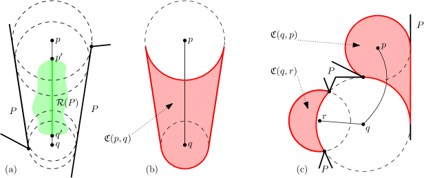
Figure 7: (a) $pq$ is a sub-arc of $\mathfrak{M}(P)$. $p^{\prime}q^{\prime}$ is the intersection of $pq$ with $\mathcal{R}(P)$. We also have $p^{\prime}q^{\prime}=\mathfrak{M}(P)\cap\mathcal{R}(P)$. (b) The cylinder $\mathfrak{C}(p,q)$ of the pair $(p,q)$ in (a). (c) Cylinders $\mathfrak{C}(q,p)$ and $\mathfrak{C}(q,r)$ illustrate the two other possible geometric shapes of a cylinder, whose boundary alternate between a part of a feature of $P$ and a circular arc.

We define a condition $G(p,q)$ as follows: Let $Q$ be a site farthest from $p$, and let $w$ be a feature of $Q$ closest to $p$. Then $G(p,q)$ is true if $w\subset\mathfrak{C}(p,q)$ or if $Q$ intersects $D_{P}(q)$. Note that $G(p,q)$ could possibly depend on the choice of $Q$ and $w$ when the farthest site or the closest feature is not unique. We will show below that this choice does not matter for the correctness of our algorithm.

We can now prove the following two lemmas:

Lemma 18.

Let $p,q$ be points on the same arc $\alpha$ of $\mathfrak{M}(P)$, such that neither $p$ nor $q$ lie in $\mathcal{R}(P)$. If $\alpha$ intersects $\mathcal{R}(P)$ between $p$ and $q$, then $G(p,q)$ and $G(q,p)$ both hold.

Proof.

Since the statement is symmetric, we only need to show $G(p,q)$. Let $Q$ be a site farthest from $p$, and let $x$ be a point between $p$ and $q$ on $\alpha$ that lies in $\mathcal{R}(P)$. This implies that $Q$ intersects $D_{\mathcal{S}}(x)=D_{P}(x)$. Since $Q$ does not intersect $D_{P}(p)$, we deduce that $Q$ intersects $\mathfrak{C}(p,q)$. If $Q$ does not lie entirely in $\mathfrak{C}(p,q)$ then, since the sites $P$ and $Q$ are disjoint, $Q$ must cross the common boundary of $\mathfrak{C}(p,q)$ and $D_{P}(q)$ (see Fig. 7(b, c)). Thus $Q$ intersects $D_{P}(q)$ and indeed $G(p,q)$ holds. ∎

Lemma 19.

Let $p,q$ be points on the same arc $\alpha$ of a tree $\mathcal{T}$ of $\mathfrak{M}(P)$ that admits no vertex in $\mathcal{R}(P)$. If neither $p$ nor $q$ lie in $\mathcal{R}(P)$ and both $G(p,q)$ and $G(q,p)$ hold, then all points in $\mathcal{T}\cap\mathcal{R}(P)$ lie on $\alpha$.

Proof.

Assume, for a contradiction, that there exists a point $x$ on $\mathcal{T}$ in $\mathcal{R}(P)$ not between $p$ and $q$ on $\alpha$; assume, without loss of generality, that $p$ lies on the path joining $x$ and $q$ in $\mathcal{T}$. Since $G(p,q)$ holds, there is a farthest site $Q\neq P$ from $p$ such that $Q$ intersects $\mathfrak{C}(p,q)$. Therefore there exists a point $y$ between $p$ and $q$ on $\alpha$ such that $y$ is closer to $Q$ than to $P$. Since $x\in\mathcal{R}(P)$ by assumption, $x$ is closer to $Q$ than to $P$. We have shown that $x$ and $y$ are closer to $Q$ than to $P$ but the point $p$, which is between $x$ and $y$ on $\mathcal{T}$, is closer to $P$ than to $Q$. This contradicts Lemma 1, and concludes the proof. ∎

Let us call an arc $\alpha$ connecting vertices $p$ and $q$ of $\mathcal{T}$ a candidate arc if $G(p,q)$ and $G(q,p)$ both hold. Lemma 19 implies immediately that if there are two candidate arcs, then $\mathcal{T}\cap\mathcal{R}(P)$ is empty, and there are no mixed vertices on $\mathcal{T}$.

Since we have point-location data structures for $\mathfrak{F}(\mathcal{S}_{1})$ and $\mathfrak{F}(\mathcal{S}_{2})$, we can test the condition $G(p,q)$ in time $O(\log n)$ for a given arc $\alpha$ in $\mathfrak{M}(P)$ and two points $p,q\in\alpha$. This allows to identify all candidate arcs in $O(m\log n)$ time, where $m$ is the complexity of $\mathcal{T}$. If there are zero or more than one candidate arcs, we can stop immediately, as there are no mixed vertices on $\mathcal{T}$.

It remains to consider the case where there is a single candidate arc $\alpha$ in $\mathcal{T}$. We again apply parametric search, using an unknown point $s^{\ast}$ in $\alpha\cap\mathcal{R}(P)$ as the query point. During the point-location query, we maintain an interval $pq$ on $\alpha$ that must contain $s^{\ast}$ (if $s^{\ast}$ exists at all). To implement a primitive query, we must determine the location of $s^{\ast}$ with respect to a comparator $\gamma$. If the current interval $pq$ on $\alpha$ does not intersect $\gamma$, we can proceed immediately, otherwise we get a sequence of points $p=x_{0},x_{1},x_{2},\dots,x_{s}=q$ on $\alpha$, where $2\leqslant s\leqslant 5$ (since there are at most four intersection points $x_{1},x_{2},\dots,x_{s-1}$ between two curves of degree at most two). We first test if some $x_{i}\in\mathcal{R}(P)$ in $O(\log n)$ time. If so, we abort the process, and use the method discussed above to find the mixed vertices on the arc between $p$ and $x_{i}$ and between $x_{i}$ and $q$. If no $x_{i}$ lies in $\mathcal{R}(P)$, we test the conditions $G(x_{i},x_{i+1})$ and $G(x_{i+1},x_{i})$ for each consecutive pair. If the conditions hold for no pair or for more than one pair, we can stop immediately, as there cannot be a point of $\mathcal{R}(P)$ on $\alpha$. If there is exactly one pair, we have found the location of $s^{\ast}$ with respect to the comparator $\gamma$, and we continue the point location query.

If both point location queries on $s^{\ast}$ in $\mathfrak{F}(\mathcal{S}_{1})$ and $\mathfrak{F}(\mathcal{S}_{2})$ terminate without encountering a point in $\mathcal{R}(P)$, the current arc $pq$ of $\alpha$ lies entirely on an arc of $\mathfrak{F}(\mathcal{S}_{1})$ and in a cell of $\mathfrak{F}(\mathcal{S}_{2})$ (assuming that $P\in\mathcal{S}_{1}$). Moreover, we get this arc and cell from the two point location queries. The two mixed vertices $s^{\ast}$ on the arc $pq$ are then both defined by the same three features that define this arc and cell, and they can be computed in constant time.

4.1.3 Avoiding randomization

Finally, we argue that, instead of using a randomized point-location data structure in the above algorithm, we can use any other data structure, such as the one of Edelsbrunner et al. [8], as long as all predicates used in the associated point-location algorithm are answered by evaluating the signs of polynomial expressions of bounded degree in the input data. If one predicate is answered by evaluating the sign of several polynomial expressions, it can be split into several predicates, each of which corresponds to exactly one polynomial expression. Then, a predicate corresponds to a polynomial expression of bounded degree that depends on the $x$ and $y$ coordinates of the query point and a set of other parameters (for instance, the coordinates of a point, or the coefficients of an implicit equation of a curve, against which the query point is tested); this expression, seen as a polynomial in $x$ and $y$, defines a curve, $\gamma$, of bounded degree. Recall now that we perform a point location query using an unknown query point $s^{\ast}$ that lies on a straight or parabolic arc. The curve $\gamma$ associated with a polynomial predicate splits this arc into a bounded number of pieces along which the sign of the polynomial is constant. To answer the query, it suffices to use the method described above on the boundary points of these pieces.

5 Concluding remarks

We have considered, in this paper, farthest-site Voronoi diagrams of $k$ disjoint connected polygonal sites in general position and of total complexity $n$. In particular, we proved that such diagrams have complexity $O(n)$ and that they can be computed in $O(n\log^{3}n)$ time.

We have seen that Voronoi regions can consist of several unbounded components. However, since the pattern $PQPQ$ cannot appear at infinity, it is always possible to connect the components of one Voronoi region by drawing non-crossing connections “at infinity,” and so we can think about Voronoi regions as being connected at infinity. This curious property can perhaps be better understood by studying the same problem on the sphere. Here the resulting structure is simpler: The bisector of two polygons is a single closed curve, and the family of bisectors of a fixed polygon $P$ with the other polygons forms a collection of pseudo-circles. (The closest-site Voronoi diagram of three disjoint polygons cannot have three vertices.) The farthest-site Voronoi region of $P$ is the intersection of the pseudo-disks that do not contain it, and is thus either empty or simply connected [16]. The $O(k)$ bound on the number of pure vertices is then a simple consequence of the planarity of this diagram. (With some care, an alternate proof of Lemma 8 based on this pseudo-disk property could be given.)

Farthest-site Voronoi diagrams are related to the function $f_{F}:x\mapsto\arg\max_{S\in\mathcal{S}}{\left(\min_{y\in S}{d(x,y)}\right)}$ which returns the farthest site to a query point. The standard closest-site Voronoi diagram corresponds to the function $x\mapsto\arg\min_{S\in\mathcal{S}}{\left(\min_{y\in S}{d(x,y)}\right)}$ which returns the closest site to a query point. Voronoi diagrams induced by other similar functions have also been considered in the literature. In particular, the diagram obtained by considering the “dual” function of $f_{F}$, that is $x\mapsto\arg\min_{S\in\mathcal{S}}{\left(\max_{y\in S}{d(x,y)}\right)}$ is the so-called Hausdorff Voronoi diagram; see [18] and references therein.

A Hausdorff diagram is typically defined for a collection of sets of points in convex position because the maximum distance from a point to a polygonal site is realized at a vertex of the polygon’s convex hull. Papadopoulou showed that the size of the Hausdorff Voronoi diagram is $\Theta(n+M)$, where $n$ is the number of points in the collection and $M$ is the number of so-called “crucial supporting segments” between pairs of “crossing sets” (a pair of sets is crossing if the convex hull boundary of their union admits more than two “supporting segments”, that is, segments joining the convex hulls of each set; such a segment is said crucial if it is enclosed in the minimum enclosing circle of each set.)

A fast parallel algorithm was obtained by Dehne et al. for the special case when $M=0$ [7]. They gave an $O((n\log^{4}n)/p)$ time parallel algorithm for the diagram construction on $p$ processors and a $O(n\log^{4}n)$ time sequential algorithm. Their algorithm is similar to ours and differs mainly is the way the purple chains are constructed. Indeed, the arcs of a Hausdorff Voronoi diagram are (straight) line segments; this permits the use of an ad hoc data structure for finding the “mixed” vertices. In contrast, arcs in a farthest-polygon Voronoi diagram can be curved and we offer a technique for computing the purple chains using parametric search, which is more efficient and more general. This generality has already found another application in the construction of farthest-site Voronoi diagrams for the geodesic distance [5]. We also believe that our technique could be applied in the sequential algorithm of Dehne et al. to improve its time complexity to $O(n\log^{3}n)$.

On the other hand, we do not provide a parallel algorithm for computing farthest-polygon Voronoi diagrams. It would be of interest to study the feasibility of applying the parallel techniques of Dehne et al. to the farthest-site Voronoi diagram computation.

References

- [1] M. Abellanas, F. Hurtado, C. Icking, R. Klein, E. Langetepe, L. Ma, B. Palop, and V. Sacristán. The farthest color Voronoi diagram and related problems. In Abstracts 17th European Workshop Comput. Geom., pages 113–116. Freie Universität Berlin, 2001.
- [2] M. Abellanas, F. Hurtado, C. Icking, R. Klein, E. Langetepe, L. Ma, B. Palop, and V. Sacristán. Smallest color-spanning objects. In Proc. 9th Annu. European Sympos. Algorithms. Lecture Notes Comput. Sci., vol. 2161, pages 278–289. Springer-Verlag, 2001.
- [3] F. Aurenhammer, R. L. S. Drysdale, and H. Krasser. Farthest line segment Voronoi diagrams. Information Processing Letters, 100:220–225, 2006.
- [4] F. Aurenhammer and R. Klein. Voronoi diagrams. In J.-R. Sack and J. Urrutia, editors, Handbook of Computational Geometry, pages 201–290. Elsevier, 2000.
- [5] S. W. Bae and K.-Y. Chwa. The geodesic farthest-site Voronoi diagram in a polygonal domain with holes. In Proc. 25th Annual Symposium on Computational Geometry, pages 198–207. ACM, 2009.
- [6] M. de Berg, O. Cheong, M. van Kreveld, and M. Overmars. Computational Geometry: Algorithms and Applications, 3rd edn. Springer-Verlag, 2008.
- [7] F. Dehne, A. Maheshwari, and R. Taylor. A coarse grained parallel algorithm for Hausdorff Voronoi diagrams. In Proc. 35th Int. Conf. on Parallel Processing (ICPP), pages 497–504. IEEE Computer Society, 2006.
- [8] H. Edelsbrunner, L. J. Guibas, and J. Stolfi. Optimal point location in a monotone subdivision. SIAM Journal on Computing, 15:317–340, 1986.
- [9] S. J. Fortune. A sweepline algorithm for Voronoi diagrams. Algorithmica, 2:153–174, 1987.
- [10] A. Hatcher. Algebraic Topology. Cambridge University Press, 2002.
- [11] D. P. Huttenlocher, K. Kedem, and M. Sharir. The upper envelope of Voronoi surfaces and its applications. Discrete Comput. Geom., 9:267–291, 1993.
- [12] S. Jadhav, A. Mukhopadhyay, and B. K. Bhattacharya. An optimal algorithm for the intersection radius of a set of convex polygons. J. Algorithms, 20:244–267, 1996.
- [13] M. van Kreveld and T. Schlechter. Automated label placement for groups of islands. In Proc. of the 22nd International Cartographic Conference (ICC2005), 2005.
- [14] N. Megiddo. Applying parallel computation algorithms in the design of serial algorithms. J. ACM, 30:852–865, 1983.
- [15] K. Mehlhorn, S. Meiser, and R. Rasch. Furthest site abstract Voronoi diagrams. Int. J. Comput. Geom. & Appl., 11:583–616, 2001.
- [16] J. Molnár. Über eine Verallgemeinerung auf die Kugelfläche eines topologischen Satzes von Helly. Acta Math. Acad. Sci., 7:107–108, 1956.
- [17] K. Mulmuley. A fast planar partition algorithm, I. J. Symbolic Comput., 10:253–280, 1990.
- [18] E. Papadopoulou. The Hausdorff Voronoi diagram of point clusters in the plane. Algorithmica, 40:63–82, 2004.
- [19] M. Sharir and P. K. Agarwal. Davenport-Schinzel Sequences and Their Geometric Applications. Cambridge University Press, 1995.