Achieving ground-state polar molecular condensates by chainwise atom-molecule adiabatic passage

Abstract

We generalize the idea of chainwise stimulated Raman adiabatic passage (STIRAP) [Kuznetsova et al. Phys. Rev. A 78, 021402(R) (2008)] to a photoassociation-based chainwise atom-molecule system, with the goal of directly converting two-species atomic Bose-Einstein condensates (BEC) into a ground polar molecular BEC. We pay particular attention to the intermediate Raman laser fields, a control knob inaccessible to the usual three-level model. We find that an appropriate exploration of both the intermediate laser fields and the stability property of the atom-molecule STIRAP can greatly reduce the power demand on the photoassociation laser, a key concern for STIRAPs starting from free atoms due to the small Franck-Condon factor in the free-bound transition.

I Introduction

A condensate of ground polar molecules with large permanent electric dipoles represents a novel state of matter with long-range and anisotropic dipole-dipole interactions that are highly amenable to the manipulation by dc and ac microwave fields zoller08am . As such, creation of such a condensate is expected to be celebrated as another milestone that promises to greatly spur activities at the forefront of physics research, particularly with respect to quantum computing and simulation demille02 and precision measurement precisionmeasurement .

The road to molecular condensation is, however, complicated by the fact that more degrees of freedom are needed to describe molecules than atoms. In particular, cooling particles by entropy removal, a direct method popular with atoms, has so far proved to be unable to lower the temperature of molecules down to the regime of quantum degeneracy. Thus, most current experimental efforts in both homonuclear homonuclear and heteronuclear Jin08 ; KKNi08 ; Ospelkaus08 ; Demille04 ; Demille05 molecules have all taken a different approach exemplified by the first experimental realization of ground polar RbCs molecules Demille05 , in which molecules are first coherently created from ultracold atoms by photoassociation (PA) Julienne06 , and are then brought down to the lower energy state by a coherent laser field (instead of by spontaneous decay Demille04 ; Deiglmayr08 ; Wang04 ). More recently, by applying a single-step stimulated Raman adiabatic passage (STIRAP)Bergmann98 onto the weakly bound Feshbach molecules, groups at JILA Jin08 ; KKNi08 ; Ospelkaus08 have successfully created an ultracold dense gas of polar ⁴⁰K⁸⁷Rb molecules.

In such schemes, there is a relatively large energy difference between the initial Feshbach and final ground molecular states.  The former, being close to the dissociation limit, is a highly delocalized state, while the latter is a tightly bound state.  It is then, in principle, difficult to locate a single excited state, capable of a large spatial overlap integral [or equivalently a good Franck-Condon (FC) factor] with both the initial and final states.  The desire to overcome this obstacle has led to the idea of stepwise STIRAP Jaksch02 ; Shapiro07 , and more recently to the idea of chainwise STIRAP Yelin08 , both of which are based on models where additional intermediate states and Raman laser fields are introduced to form a chain of $\Lambda$ systems multilevel ; Vitanov98 .  In these STIRAPs, the two lower states within each sub-$\Lambda$ system are far closer in energy than the initial and final states, thereby greatly boosting the chance of locating an excited state capable of a large FC transition to both lower states.  In contrast to a stepwise STIRAP, which employs a series of STIRAPs to move molecules one step at a time down each lower intermediate state, a chainwise STIRAP applies a single STIRAP between the initial and final lasers to transfer molecules, while uses relatively high intermediate cw lasers to keep all the lower intermediate states virtually unoccupied.  This latter method eliminates the opportunities for molecules to inherit decoherence from the unstable lower intermediate states, and is clearly an improvement over the former as far as the ability to preserve the phase-space density is concerned.

The focus of this paper is on the coupled multilevel atomic-molecular condensate systems where the role of the initial transition is played by photoassociation. (An example is provided in Fig. 1, which will be described in detail in the next section.)  Our goal is to develop a generalized chainwise STIRAP founded on the concept of atom-molecule dark state, a coherent population trapping (CPT) superposition between stable ground species Mackie00 ; Ling .  This scheme has several attractive properties. First, atoms are directly converted into ground molecules.  Thus, the loss of atoms typically associated with the initial preparation of Feshbach molecules Jin08 ; Thalhammer06 is never an issue here.  Second, pulses of longer durations can be employed to meet the adiabatic condition; we can do so because the atom-molecule dark state is far more stable than the molecular dark state, where the initial state is highly unstable compared to the ground (atom or molecule) states. Finally, the use of intermediate lasers presents us with a new control knob inaccessible to typical three-level models. It is the purpose of this paper to show that an appropriate exploration of both the intermediate laser fields and the stability property of the dark state can greatly reduce the power demand for the PA laser needed for an efficient conversion. This along with other efforts involving the use of Feshbach resonance Feshbach may help to combat the weakness in photoassociation, a key concern to STIRAPs starting from free atoms due to the free-bound FC factor being typically very small.

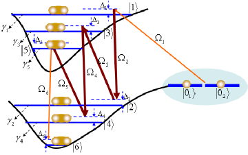
Figure 1: (Color online) A schematic of a chainwise STIRAP.

Our paper is organized as follows. In Sec. II, we describe our model and the underlying mean-field equations and provide the rationale that justifies the implementation of chainwise STIRAP in our model. In Sec. III, we derive a set of linearized equations around the time-dependent CPT solution and obtain an adiabatic condition via a state expansion over a set of orthonormal base vectors provided in Appendix B. In Sec. IV, we apply this adiabatic theorem to facilitate our numerical studies of the examples that serve to illustrate the main physics outlined in the previous paragraph.  Finally, a summary is given in Sec. V.

II Model and CPT State

Figure 1 is the energy schematic diagram for a minimum model that is capable of illustrating all the main points that we want to convey in this paper. A laser field associates atoms from two distinct species of states $\left|0_{1}\right\rangle$ and $\left|0_{2}\right\rangle$ into molecules of state $\left|1\right\rangle$ in the excited electronic manifold with a coupling strength $\Omega_{1}$ proportional to the laser field and the free-bound FC factor. Simultaneously, a series of laser fields of (molecular) Rabi frequency $\Omega_{i}$ $\left(i\geq 2\right)$ is applied to move the molecules from the excited to the ground state $\left|6\right\rangle$ via additional intermediate energy states.  In our notation, a molecular state $\left|i\right\rangle$ ($i=1,2,\cdots,6$) is coupled to the atomic states via an $i$-photon process characterized with an $i$-photon detuning $\Delta_{i}$ defined, respectively, as $\Delta_{1}=\omega_{1}-E_{1}/\hbar,$ $\Delta_{2}=\left(\omega_{1}-\omega_{2}\right)-E_{2}/\hbar$, $\Delta_{3}=\left(\omega_{1}-\omega_{2}+\omega_{3}\right)-E_{3}/\hbar,$ etc., where $\omega_{i}$ stands for the (temporal) frequency of the laser field with Rabi frequency $\Omega_{i}$, and $E_{i}$ for the energy of molecular state $\left|i\right\rangle$ relative to the free atomic energy level.  Further, intermediate states $\left|i\right\rangle$ ($i=1,2,\cdots,5)$ are assumed to be unstable; for each intermediate state $\left|i\right\rangle$, a decay rate $\gamma_{i}$ is introduced to describe phenomenologically the loss of its molecules due to various incoherent processes.

As a proof of principle, we consider, in this paper, a uniform condensate system with a total atom number density $n$ and describe such a system with a set of field operators $\hat{\Psi}_{i}$, where $\hat{\Psi}_{i}$ is the operator for annihilating a bosonic particle in condensate state $\left|i\right\rangle$.  By following the mean-field treatment of photoassociation at zero temperature Heinzen00 in which each $\hat{\Psi}_{i}$ is treated as a c number $\Psi_{i}$, we obtain, from the Heisenberg’s equations for operators $\hat{\Psi}_{i}$, a set of coupled Gross-Pitaevskii’s equations for the normalized condensate fields $\psi_{i}=\Psi_{i}/\sqrt{n}$:

$$i\dot{\psi}_{0_{1}} =\frac{\Omega_{1}}{2}\psi_{0_{2}}^{\ast}\psi_{1},$$ (1a)

$$i\dot{\psi}_{0_{2}} =\frac{\Omega_{1}}{2}\psi_{0_{1}}^{\ast}\psi_{1},$$ (1b)

$$i\dot{\psi}_{1} =\left(\Delta_{1}-i\gamma_{1}\right)\psi_{1}+\frac{\Omega_{1}}{2}\psi_{0_{1}}\psi_{0_{2}}+\frac{\Omega_{2}}{2}\psi_{2},$$ (1c)

$$i\dot{\psi}_{i} =\left(\Delta_{i}-i\gamma_{i}\right)\psi_{i}+\frac{\Omega_{i}}{2}\psi_{i-1}+\frac{\Omega_{i+1}}{2}\psi_{i+1}\text{, }i=2,3,\cdots 5,,$$ (1d)

$$i\dot{\psi}_{6} =\Delta_{6}\psi_{6}+\frac{\Omega_{6}}{2}\psi_{5}.$$ (1e)

where the molecular Rabi frequencies

$$\Omega_{1} =\sqrt{2}\sqrt{n}\bar{\Omega}_{1}^{\left(el\right)}\left\langle v_{1}|v^{\left(0\right)}\right\rangle,$$ (2a)

$$\Omega_{i} =\bar{\Omega}_{i}^{\left(el\right)}\left\langle v_{i}|v_{i+1}\right\rangle,\text{ }i=2,3,\cdots 6,$$ (2b)

are expressed in terms of the mean electronic Rabi frequency $$\bar{\Omega}_{i}^{\left(el\right)} \left\langle v_{1}|v^{\left(0\right)}\right\rangle \left\langle v_{i}|v_{i+1}\right\rangle v_{i} v^{\left(0\right)} R \left|i\right\rangle \left|0_{1}\right\rangle \left|0_{2}\right\rangle s \Omega_{3}=\Omega_{5}\equiv\Omega_{o} \Omega_{2}=\Omega_{4}\equiv\Omega_{e} o e$$, the free-bound FC factor , and the bound-bound FC factor , where and are the stationary wave functions (of interatomic distance ) for a bound molecular state and a pair of atoms in states and , respectively Drummond02 ; Naidon03 .  In arriving at Eqs. (1), without the loss of the main physics, we have followed Refs. Jin08 ; Yelin08 and ignored all the two-body -wave collisions.  Further, in order to better illustrate the essential physics, we will limit our study to a model in which and , where subscript and stand for the intermediate lasers of odd and even indices, respectively.

Before moving ahead, we note that Jaksch et. al. Jaksch02 have identified a set of rovibrational levels from $X^{1}\Sigma_{g}^{+}$ (ground) and $A^{1}\Sigma_{u}$ (excited) electronic manifolds to implement the homonuclear version of the model in Fig. 1 for producing $Rb_{2}$ molecules in the ground state $X^{1}\Sigma_{g}^{+}(v=0,j=0)$ [=$\left|6\right\rangle$].  It is true that in order to arrive at a similar set of pathways for the heteronuclear model, one must perform a careful analysis of experimental spectroscopic data and possibly, ab initia calculation of various overlap integrals [FC factors defined in Eqs. (2)] Deb03 ; Azizi04 ; Bigelow07 .  However, the selection rules for heteronuclear molecules are actually more relaxed; the heteronuclear molecular orbitals do not have g/u symmetry, and the number of possible transitions between the free atomic and the ground molecular state is thus doubled.  As a result, it is not difficult to see that such a model can be easily generalized from homonuclear to heteronulcear molecules.

By ignoring the decays (see the justification that follows) and subjecting our system to the conservation of total particle number,

$$\psi_{0_{1}}^{2}+\psi_{0_{2}}^{2}+2\sum_{i=1}^{6}\psi_{i}^{2}=1$$ (3)

and that of atomic population difference: $\psi_{0_{1}}^{2}-\psi_{0_{2}}^{2}\equiv$ $0$ (or $\psi_{0_{1}}^{2}=\psi_{0_{2}}^{2}\equiv\psi_{0}^{2}$ for a balanced model), we find that under the conditions of two-, four-, and six-photon resonance, namely, $\Delta_{2}=\Delta_{4}=\Delta_{6}=0,$ the system at steady state supports a superposition involving all the lower states with the following amplitude distribution (see Appendix A for a detailed derivation):

$$\varphi_{0} =\frac{1}{\sqrt{1+\sqrt{1+2\left(\alpha^{2}\Omega_{1}/\Omega_{6}\right)^{2}}}},$$ (4a)

$$\varphi_{2} =-\xi\varphi_{0}^{2},\varphi_{4}=\xi\alpha\varphi_{0}^{2},\varphi_{6}=-\alpha^{2}\frac{\Omega_{1}}{\Omega_{6}}\varphi_{0}^{2},$$ (4b)

$$\varphi_{1} =\varphi_{3}=\varphi_{5}=0,$$ (4c)

where $$\alpha=\Omega_{o}/\Omega_{e} \xi=\Omega_{1}/\Omega_{e} \xi \left(\Omega_{o},\Omega_{e}\right) \left(\Omega_{1},\Omega_{6}\right) \left|2\right\rangle \left|4\right\rangle \xi \xi\ll 1 \left|2\right\rangle \left|4\right\rangle \alpha \Omega_{1}/\Omega_{6} \alpha^{2}\Omega_{1} \Omega_{1} \alpha \alpha$$, . In arriving at Eq. (4), we have only retained the leading order term in , assuming that the intermediate fields are far stronger than the initial and final fields Vitanov98 ; Yelin08 . (Unless stated otherwise, a similar perturbative interpretation applies to all the other results.)  It needs to be stressed that Eq. (4) is derived when all the decays are ignored.  As a result, it represents a steady state (or CPT state) of Eqs. (1) (where all the decay rates are included) only when it does not involve any unstable states.  The only unstable states in Eq. (4) are the lower intermediate states: and whose amplitudes scale as .  Thus, it is in the limit when states and remain virtually empty that this superposition can be truly called a “CPT” or “dark” state.  Also evident is that in the same limit and for a fixed , the initial and final populations are solely determined by the ratio . This lays the foundation for converting all the atoms into the ground molecules by a chainwise STIRAP where a counterintuitive pulse sequence is maintained only between the initial and final laser fields. Another important feature is that the initial and final populations are function of so that the change by can also be accomplished by varying . However, the full impact of on the STIRAP has to wait until we know the adiabatic condition.

III Adiabatic Condition

To obtain the adiabatic condition, we linearize Eqs. (1) around the instantaneous CPT state $\varphi_{i}\left(t\right)$ according to $\psi_{i}\left(t\right)=\varphi_{i}\left(t\right)+\delta\psi_{i}\left(t\right)$, where $\delta\psi_{i}\left(t\right)$ is the small perturbation, and $\varphi_{i}\left(t\right)$ are Eqs. (4) when $\Omega_{i}$ are replaced with their instantaneous values $\Omega_{i}\left(t\right)$ at time $t$.  This procedure results in a matrix equation for the ket $\left|\delta\psi\right\rangle=\left(\delta\psi_{0_{1}},\delta\psi_{0_{2}},\delta\psi_{1},\cdots,\delta\psi_{6}\right)^{T}$:

$$i\frac{d}{dt}\left|\delta\psi\right\rangle=\left(\mathbf{M}-i\mathbf{\gamma}\right)\left|\delta\psi\right\rangle-i\left|\dot{\varphi}\right\rangle,$$ (5)

where

$$\mathbf{M}=\frac{1}{2}\left(\begin{array}[c]{cccccccc}0&0&\Omega_{1}^{\prime}&0&0&0&0&0\\ 0&0&\Omega_{1}^{\prime}&0&0&0&0&0\\ \Omega_{1}^{\prime}&\Omega_{1}^{\prime}&2\Delta_{1}&\Omega_{2}&0&0&0&0\\ 0&0&\Omega_{2}&0&\Omega_{3}&0&0&0\\ 0&0&0&\Omega_{3}&2\Delta_{3}&\Omega_{4}&0&0\\ 0&0&0&0&\Omega_{4}&0&\Omega_{5}&0\\ 0&0&0&0&0&\Omega_{5}&2\Delta_{5}&\Omega_{6}\\ 0&0&0&0&0&0&\Omega_{6}&0\end{array}\right),\mathbf{\gamma}=\left(\begin{array}[c]{cccccccc}0&0&0&0&0&0&0&0\\ 0&0&0&0&0&0&0&0\\ 0&0&\gamma_{1}&0&0&0&0&0\\ 0&0&0&\gamma_{2}&0&0&0&0\\ 0&0&0&0&\gamma_{3}&0&0&0\\ 0&0&0&0&0&\gamma_{4}&0&0\\ 0&0&0&0&0&0&\gamma_{5}&0\\ 0&0&0&0&0&0&0&0\end{array}\right),\left|\dot{\varphi}\right\rangle=\left(\begin{array}[c]{c}\dot{\varphi}_{0}\\ \dot{\varphi}_{0}\\ 0\\ \gamma_{2}\varphi_{2}+\dot{\varphi}_{2}\\ 0\\ \gamma_{4}\varphi_{4}+\dot{\varphi}_{4}\\ 0\\ \dot{\varphi}_{6}\end{array}\right),$$ (6)

with $\Omega_{1}^{\prime}=\varphi_{0}\Omega_{1}$.  Following the standard procedure Han , we expand $\left|\delta\psi\left(t\right)\right\rangle=\sum c_{i}\left(t\right)\left|\lambda_{j}\left(t\right)\right\rangle$ in the space spanned by the instantaneous collective modes $\left|\lambda_{j}\left(t\right)\right\rangle$ defined by

$$\mathbf{M}\left|\lambda_{j}\left(t\right)\right\rangle=\lambda_{j}\left(t\right)\left|\lambda_{j}\left(t\right)\right\rangle.$$ (7)

In this new basis and under the condition that $\left\langle\lambda_{i}\right|\mathbf{\dot{M}}\left|\lambda_{j}\right\rangle/\left|\lambda_{j}-\lambda_{i}\right|<<1$ $\left(\lambda_{i}\neq\lambda_{j}\right)$, Eq. (5) becomes

$$i\frac{dc_{i}}{dt}=\lambda_{i}c_{i}-i\sum_{j}\left\langle\lambda_{i}\right|\mathbf{\gamma}\left|\lambda_{j}\right\rangle c_{j}-i\left\langle\lambda_{i}|\dot{\varphi}\right\rangle$$ (8)

and can be put in a form convenient for us to estimate the magnitudes of various $c_{i}$ due to the time variation of the CPT state $\left|\dot{\varphi}\right\rangle$, or in another words, to arrive at the adiabatic condition.  (Note that whenever confusion is unlikely, we omit argument $t$ to time-dependent variables.)

Thus, we see that the most crucial step in developing an adiabatic theorem is to determine from Eq. (7) a set of base vectors  $\left|\lambda_{j}\right\rangle$ upon which we can expand $\left|\delta\psi\left(t\right)\right\rangle$.  As this step itself can often be quite involved, we focus on a simplified model with $\Delta_{1}=\Delta_{3}=\Delta_{5}=0$.   As we show in Appendix B, for this special model and in the limit $\xi\ll 1$, we can apply perturbation theory to obtain simple analytical solutions from Eq. (7).  In what follows, we simply quote the relevant results and refer interested readers to Appendix B for details.  In a nutshell, the collective modes are found to consist of $\lambda_{1,2}=0$ [same as $\bar{\lambda}_{1,2}$ in Eq. (24)] with a double degeneracy, a set of “soft” modes $\lambda_{3,4}=\pm\Omega_{eff}/\left(2\beta\right)$ [same as $\bar{\lambda}_{3,4}$ in Eq. (24)] that scale as $\left(\Omega_{1}^{\prime}\text{ and }\Omega_{6}\right)$, where $\Omega_{eff}=\sqrt{2\Omega_{1}^{\prime 2}\alpha^{4}+\Omega_{6}^{2}}$ and $\beta=\sqrt{1+\alpha^{2}+\alpha^{4}}$, and two sets of “stiff” modes $\lambda_{5,6}=\pm 0.5\Omega_{e}\sqrt{1+\alpha+\alpha^{2}}$ [same as $\lambda_{5,6}^{\left(0\right)}$ in Eq. (19b)] and $\lambda_{7,8}=\pm 0.5\Omega_{e}\sqrt{1-\alpha+\alpha^{2}}$ [same as $\lambda_{7,8}^{\left(0\right)}$ in Eq. (19c)] that scale as $\Omega_{e}$ and are larger than the “soft” modes by a factor of $\xi^{-1}$. Each set of nondegenerate modes is symmetrically displaced with respect to the $0$ modes, and the appearance of the negative modes is expected because the CPT state is not a thermodynamical ground state.

The 0 mode being a doublet distinguishes the heteronuclear model Jing08 from its homonuclear counterpart which only supports a single 0 mode Han . In general, due to the ground intermediate states being unstable, the two modes here are both unstable, in contrast to the dark state in a typical three-level system, which is a stable superposition, completely isolated from other unstable states. However, by choosing the two modes in the orthonormal form

$$\left|\lambda_{1}\right\rangle =\frac{1}{\sqrt{2}}\left(-1,1,0,0,0,0,0,0\right)^{T},$$ (9a)

$$\left|\lambda_{2}\right\rangle =\frac{\left(-\Omega_{6},-\Omega_{6},0,2\xi^{\prime}\Omega_{6},0,-2\alpha\xi^{\prime}\Omega_{6},0,2\alpha^{2}\Omega_{1}^{\prime}\right)^{T}}{\sqrt{2}\Omega_{eff}},$$ (9b)

where $$\left|\lambda_{1}\right\rangle \left|\lambda_{2}\right\rangle \xi^{\prime}=\Omega_{1}^{\prime}/\Omega_{e} \xi\ll 1 \xi^{\prime}=\varphi_{0}\xi \left|\lambda_{1}\right\rangle \left|\lambda_{2}\right\rangle$$ is exact while is correct up to the first order in which scales as [see the discussion bellow Eqs. (4)] because , we find that is completely decoupled from other states as in a true dark state while couples to other states with strengths that are at the same order of magnitude as its decay rate,

$$\left\langle\lambda_{2}\right|\mathbf{\gamma}\left|\lambda_{2}\right\rangle=2\left(\gamma_{2}+\alpha^{2}\gamma_{4}\right)\xi^{\prime 2}\Omega_{6}^{2}/\Omega_{eff}^{2}\equiv 1/\tau_{0}.$$ (10)

The result in Eq. (10) corroborates our intuition that the use of relatively high intermediate laser fields can indeed make the lifetime of our CPT state, $\tau_{0}$, far longer than those of the lower intermediate states.  Clearly, in order to justify the use of the CPT state in Eqs. (4) as the adiabatic state for a STIRAP process, we must design the STIRAP in such a fashion that it is slow compared with the periods of the nonzero modes but fast compared with $\tau_{0}$, the lifetime of the CPT state.

As a result, we consider all the coupling coefficients $\left\langle\lambda_{2}\right|\mathbf{\gamma}\left|\lambda_{i}\right\rangle$ involving $\left|\lambda_{2}\right\rangle$ weak and ignore them from Eqs. (8).  In addition, we also ignore all the stiff modes, because they are $\xi^{-1}$ times more difficult to populate than the soft modes, whose eigenvectors are given by

$$\left|\lambda_{3,4}\right\rangle=\frac{1}{\sqrt{2}}\left(\frac{\alpha^{2}\Omega_{1}^{\prime}}{\Omega_{eff}},\frac{\alpha^{2}\Omega_{1}^{\prime}}{\Omega_{eff}},\pm\frac{\alpha^{2}}{\beta},0,\mp\frac{\alpha}{\beta},0,\pm\frac{1}{\beta},\frac{\Omega_{6}}{\Omega_{eff}}\right)^{T}.$$ (11)

Under these conditions, Eqs. (8) are simplified into

$$\left(i\lambda_{3}+\left\langle\lambda_{3}\right|\mathbf{\gamma}\left|\lambda_{3}\right\rangle\right)c_{3}+\left\langle\lambda_{3}\right|\mathbf{\gamma}\left|\lambda_{4}\right\rangle c_{4} =-\left\langle\lambda_{3}|\dot{\varphi}\right\rangle,$$ (12a)

$$\left\langle\lambda_{3}\right|\mathbf{\gamma}\left|\lambda_{4}\right\rangle c_{3}+\left(i\lambda_{4}+\left\langle\lambda_{4}\right|\mathbf{\gamma}\left|\lambda_{4}\right\rangle\right)c_{4} =-\left\langle\lambda_{4}|\dot{\varphi}\right\rangle.$$ (12b)

where we have ignored $$\dot{c}_{3,4}\, \lambda_{3,4}$$assuming that they are sufficiently small compared to in the adiabatic limit.

Finally, with the help of Eqs. (6) and (11), we find from Eqs. (12) that to a good approximation, the adiabatic parameter Han

$$r=\sqrt{\left|c_{3}\right|^{2}+\left|c_{4}\right|^{2}}/2$$ (13)

can be estimated according to

$$r=\frac{\sqrt{4\gamma_{eff}^{2}+\lambda^{2}}\alpha^{2}\dot{\chi}/\sqrt{2}}{\sqrt{2}\lambda^{2}\left(1+2\alpha^{4}\chi^{2}\right)^{1/4}\left(1+\sqrt{1+2\alpha^{4}\chi^{2}}\right)}\ll 1,$$ (14)

where $\chi=\Omega_{1}/\Omega_{6}$, $\lambda=$ $\Omega_{eff}/\left(2\beta\right),$ and $\gamma_{eff}=\left(\alpha^{4}\gamma_{1}+\alpha^{2}\gamma_{3}+\gamma_{5}\right)/\left(2\beta^{2}\right)$.

IV Discussion

In what follows, we seek to gain from the $r$ value in Eq. (14) insights into the parameters, especially, $\alpha$, that optimize the final conversion efficiency. In a dynamical process where the $r$ value varies with time, we find the $r$ value evaluated at time $t_{s}$ to be a good figure of merit that distinguishes different STIRAPs, where $t_{s}$ is the time when about 50% atoms would be converted into molecules if the system were to follow the CPT state. With $t_{s}$ defined above and the Gaussian pulses defined below, we find

$$t_{s}=\frac{T^{2}}{2\left(t_{1}-t_{6}\right)}\ln\left(\frac{2\Omega_{6}^{0}}{\alpha^{2}\Omega_{1}^{0}}\right)+\frac{t_{1}+t_{6}}{2},$$

where $T$, $t_{1,6}$, and $\Omega_{1,6}^{0}$ are, respectively, the width, peak times, and peak strengths of the Gaussian pulses: $\Omega_{1,6}\left(t\right)=\Omega_{1,6}^{0}\exp[-\left(t-t_{1,6}\right)^{2}/T^{2}]$. In all the calculations, $\gamma_{1,3,5}=10^{7}$ s^-1, $\gamma_{2,4}=10^{4}$ s${}^{-1},$ $t_{1}=2.5T,$ $t_{6}=1.0T$, $\Omega_{1}^{0}=3.3\times 10^{6}$ s${}^{-1},$ $\Omega_{e}=2\times 10^{8}$ s^-1, and $\Omega_{6}^{0}=8\times 10^{7}$ s^-1. Note that although in theory high adiabaticity can always be gained at the expense of a large $\Omega_{1}^{0}$, in practice, $\Omega_{1}^{0}$ is quite limited due to the relative weakness in photoassociation. For this reason, we have chosen $\Omega_{1}^{0}$ to be much weaker than $\Omega_{6}^{0}$ ($\Omega_{1}^{0}\approx\Omega_{6}^{0}/24$).  At such $\Omega_{1}^{0}$, we find, using $n=10^{20}m^{-3}$ and $\mu=4.48\times 10^{-26}kg$ (reduced mass of $K$ and $Rb$ atoms), that $\Omega_{1}^{0}/\omega_{\rho}=131,$ where $\omega_{\rho}=\hbar n^{2/3}/2\mu$ Javanainen02 .  In a STIRAP process, due to quantum interference, the molecular population in state $\left|1\right\rangle$ remains extremely small so that even when $\Omega_{1}^{0}/\omega_{\rho}$ is in the order of 10², rogue photodissociation of molecules in state $\left|1\right\rangle$ is shown to produce a negligible fraction of noncondensate atom pairs Mackie04 .  As a result, we ignore the rogue photodissociation in this work.

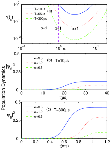
Figure 2: (Color online) (a) The $r$ value at $t_{s}$ as a function of $\alpha$ under different $T$. The population dynamics with (b) $T=10$ $\mu s$ and (c) $T=300$ $\mu s$ for different $\alpha$. Other parameters are defined in the text.

Figure 2(a) illustrates how the $r$ value at $t_{s}$ changes with $\alpha$ under different $T$. The most interesting feature here is that, for a given $T$, the $r$ value is quite high on the side of $\alpha<1$ (the left side of the dashed vertical line $\alpha=1$), but significantly smaller within certain region on the side of $\alpha>1$. As a result, we see in Fig. 2(b) with $T=10$ $\mu s$ that when $\alpha$ changes from 0.5 to 3.8 (at which, $r$ value is near minimum), the conversion efficiency $\eta[=2\psi_{6}^{2}\left(\infty\right)]$ increases from 1.8% to 22.6%, a trend consistent with Fig. 2(a) with $T=10$ $\mu s$. But, we caution that no efficiencies significantly higher than 22.6% are possible in this case by further raising the $\alpha$ value because the $r$ value actually increases with $\alpha$ when $\alpha$ is sufficiently large according to Fig. 2(a); we trace this to the fact that unlike the CPT state in Eq. (4), $\lambda$ and $\gamma_{eff}$ and hence the adiabatic condition in Eq. (14) do not scale as $\alpha^{2}\Omega_{1}$.

An important point to make is that were the lifetime of the dark state limited to the order of $10$ $\mu s$, a higher efficiency would indeed have to come at the expense of a higher PA laser power. This, however, is not needed owing to another important virtue of our system - the stability of our CPT state, whose lifetime can be made much longer than those of the lower states in the ground electronic manifold. This, therefore, affords us with a plenty of room to increase efficiency by using pulses with longer durations rather than higher powers. Indeed, the population dynamics in Fig. 2(c) with a much longer pulse ($T=300$ $\mu$s$)$ demonstrates, in addition to a trend same as in Fig. 2(b), a dramatic increase in the maximum efficiency, which can now reach more than 85%.

To estimate the required power on the photoassociation laser field, we consider heteronuclear molecules involving $Rb$ atoms, for example, $KRb$ Wang04 and $RbCs$ Demille05 .  The free-bound FC factor for heteronuclear molecules is expected to be smaller than that for their homonuclear counterparts because the excited potential at large internuclear distance $R$ for the heteronuclear molecules is dominated by the van der Waals potential (R^-6) and thus has a shorter range than that for the homonuclear molecules, which is dominated by the resonant dipole-dipole interaction (R^-3).  An encouraging news according to ab initia calculations in Refs. Azizi04 ; Ghosal09 is that the former is only slightly smaller than the latter.  As a result, in our estimation, we choose a free-bound FC factor $\left\langle v_{1}|v^{\left(0\right)}\right\rangle=3\times 10^{-14}$ m^3/2 several times smaller than that of $Rb_{2}$ molecules, which can be on the order of 10^-13m^3/2 (for $n=10^{20}$ m^-3) according to Naidon and Masnou-Seeuws Naidon03 .  Finally, using 1.6 $ea_{0}$ as the atomic dipole moment Tiesinga03 with $e$ the electron charge and $a_{0}$ the Bohr radius, we estimate the peak PA laser intensity to be $3$.$8\times 10^{3}$ W/cm².  This admittedly high (and yet attainable) intensity can be put in perspective by comparison with the case where $T=10$ $\mu$s and $\alpha=1$, where an intensity of more than $100$ times higher is needed to achieve the same level of high efficiency [in Fig. 2(c) with $\alpha=3.8$].

V Summary

In summary, we have generalized the chainwise STIRAP from pure molecular to coupled atomic-molecular systems. In addition to the known advantages, for example, the increased chance to locate pairs of Raman transitions with large FC factors, we have uncovered additional virtues. In particular, $\alpha$, a ratio between intermediate laser fields, was found to serve as a robust experimental control knob, inaccessible to the usual three-level systems. This control knob together with the stability of the atom-molecule dark state may bring us one step closer to overcome the PA weakness, so that the ground polar molecules can be created directly from degenerate atomic gases in a manner that preserves the phase-space density.

VI Acknowledgement

This work is supported by the US National Science Foundation (H.Y.L), the U.S. Army Research Office (H.Y.L.), and the National Natural Science Foundation of China under Grant No. 10588402, the National Basic Research Program of China (973 Program) under Grant No. 2006CB921104, the Program of Shanghai Subject Chief Scientist under Grant No. 08XD14017, and the Program for Changjiang Scholars and Innovative Research Team in University, Shanghai Leading Academic Discipline Project under Grant No. B480 (W.Z.).

Appendix A

This appendix provides the steps that we take to arrive at Eqs. (4). We begin with Eqs. (1) at steady state, where the derivatives on the left-hand sides are all set to zero.  Next, we ignore all the decays as well as all the excited populations $\left(\psi_{1}=\psi_{3}=\psi_{5}=0\right)$.  We then see that the equations for $\psi_{2},\psi_{4}$, and $\psi_{6}$ lead to the CPT condition: $\Delta_{2}=\Delta_{4}=\Delta_{6}=0$, while the rest of equations are simplified to

$$-\xi\psi_{0_{1}}\psi_{0_{2}} =\psi_{2},$$ (15a)

$$-\alpha\psi_{2} =\psi_{4},$$ (15b)

$$-\frac{\Omega_{o}}{\Omega_{6}}\psi_{4} =\psi_{6}.$$ (15c)

where as in the main text we have made the use of $$\Omega_{2}=\Omega_{4}=\Omega_{e}, \Omega_{3}=\Omega_{5}=\Omega_{o} \alpha=\Omega_{o}/\Omega_{e} \xi=\Omega_{1}/\Omega_{e} \psi_{0_{1}}^{2}=\psi_{0_{2}}^{2}\equiv\psi_{0}^{2} \psi_{2}=-\xi\psi_{0}^{2} \psi_{4}=\alpha\xi\psi_{0}^{2} \psi_{6}=-\left(\Omega_{o}/\Omega_{6}\right)\alpha\xi\psi_{0}^{2}$$ , and .  For a balanced system with , we find from Eqs. (15) that , , and , which, when combined with the particle number conservation in Eq. (3), gives rise to

$$\varphi_{0}^{2} =\frac{1}{1+\sqrt{1+2\left(1+\alpha^{2}\right)\xi^{2}+2\left(\alpha^{2}\Omega_{1}/\Omega_{6}\right)^{2}}},$$

$$\varphi_{2} =-\xi\varphi_{0}^{2},\varphi_{4}=\xi\alpha\varphi_{0}^{2},\varphi_{6}=-\alpha^{2}\frac{\Omega_{1}}{\Omega_{6}}\varphi_{0}^{2}.$$

Clearly, we see that up to the first order in $\xi$, Eqs. (15) become Eqs. (4) in the main text.

Appendix B

In this appendix, we show how to obtain from Eq. (7) the eigenvalues and eigenvectors (that are needed to derive the adiabatic condition) in the limit of $\xi\ll 1$ for the special case of $\Delta_{1,3,5}=0$.  To begin, we divide $\mathbf{M}$ in Eq. (6) into two parts:

$$\mathbf{M=M}_{0}+\mathbf{M}^{\prime}$$ (16)

where

$$\mathbf{M}_{0}=\frac{1}{2}\left(\begin{array}[c]{cccccccc}0&0&0&0&0&0&0&0\\ 0&0&0&0&0&0&0&0\\ 0&0&0&\Omega_{e}&0&0&0&0\\ 0&0&\Omega_{e}&0&\Omega_{o}&0&0&0\\ 0&0&0&\Omega_{o}&0&\Omega_{e}&0&0\\ 0&0&0&0&\Omega_{e}&0&\Omega_{o}&0\\ 0&0&0&0&0&\Omega_{o}&0&0\\ 0&0&0&0&0&0&0&0\end{array}\right),\mathbf{M}^{\prime}=\frac{1}{2}\left(\begin{array}[c]{cccccccc}0&0&\Omega_{1}^{\prime}&0&0&0&0&0\\ 0&0&\Omega_{1}^{\prime}&0&0&0&0&0\\ \Omega_{1}^{\prime}&\Omega_{1}^{\prime}&0&0&0&0&0&0\\ 0&0&0&0&0&0&0&0\\ 0&0&0&0&0&0&0&0\\ 0&0&0&0&0&0&0&0\\ 0&0&0&0&0&0&0&\Omega_{6}\\ 0&0&0&0&0&0&\Omega_{6}&0\end{array}\right).$$ (17)

Here, $\mathbf{M}_{0}$ is an unperturbed part including all the intermediate Rabi frequencies $\Omega_{o}$ and $\Omega_{e}$, while $\mathbf{M}^{\prime}$, consisting of only the initial and final fields $\Omega_{1}^{\prime}$ and $\Omega_{6}$, can be regarded as a perturbation to $\mathbf{M}_{0}$ in the limit of $\xi\ll 1$.  Next, we determine from the equation

$$\mathbf{M}_{0}\left|\lambda_{j}^{\left(0\right)}\right\rangle=\lambda_{j}^{\left(0\right)}\left|\lambda_{j}^{\left(0\right)}\right\rangle$$ (18)

eigenvalues $\lambda_{j}^{\left(0\right)}$ and eigenstates $\left|\lambda_{j}^{\left(0\right)}\right\rangle$ of the unperturbed part $\mathbf{M}_{0}$.  We find that $\lambda_{j}^{\left(0\right)}$ take the following values:

$$\lambda_{1,2,3,4}^{\left(0\right)}=0,$$ (19a)

$$\lambda_{5,6}^{\left(0\right)}=\frac{\pm\Omega_{e}\sqrt{1+\alpha+\alpha^{2}}}{2},$$ (19b)

$$\lambda_{7,8}^{\left(0\right)}=\frac{\pm\Omega_{e}\sqrt{1-\alpha+\alpha^{2}}}{2}.$$ (19c)

The zero eigenvalue has a four-fold degeneracy, and the corresponding (orthonormalized) eigenstates are found from Eq. (18) to take the form

$$\left|\lambda_{1}^{\left(0\right)}\right\rangle =(1,0,0,0,0,0,0,0)^{T},$$ (20a)

$$\left|\lambda_{2}^{\left(0\right)}\right\rangle =(0,1,0,0,0,0,0,0)^{T},$$ (20b)

$$\left|\lambda_{3}^{\left(0\right)}\right\rangle =(0,0,0,0,0,0,0,1)^{T},$$ (20c)

$$\left|\lambda_{4}^{\left(0\right)}\right\rangle =(0,0,\frac{\alpha^{2}}{\beta},0,-\frac{\alpha}{\beta},0,\frac{1}{\beta},0)^{T},$$ (20d)

where $$\beta=\sqrt{1+\alpha^{2}+\alpha^{4}} \mathbf{M}^{\prime} \lambda_{5,6}^{\left(0\right)} \lambda_{7,8}^{\left(0\right)} \Omega_{e} \mathbf{M}^{\prime} \mathbf{M}^{\prime}$$.  This degeneracy, however, can be partially lifted by the perturbation as we will show shortly.   and are proportional to and are far larger in magnitude than those split from the zero eigenvalue by ; the modes associated with the former eigenvalues are far more difficult to populate than those associated with the latter eigenvalues.  Thus, it suffices, for our purpose, that we only focus on the eigensubspace spanned by the four base vectors in Eqs. (20), in which in Eq. (17) has the following matrix representation

$$\mathbf{M}^{\prime}=\frac{1}{2\beta}\left(\begin{array}[c]{cccc}0&0&0&\Omega_{1}^{\prime}\alpha^{2}\\ 0&0&0&\Omega_{1}^{\prime}\alpha^{2}\\ 0&0&0&\Omega_{6}\\ \Omega_{1}^{\prime}\alpha^{2}&\Omega_{1}^{\prime}\alpha^{2}&\Omega_{6}&0\end{array}\right)$$ (21)

where the use of $\mathbf{M}_{ij}^{\prime}=\left\langle\lambda_{i}^{\left(0\right)}\right|\mathbf{M}^{\prime}\left|\lambda_{j}^{\left(0\right)}\right\rangle$ has been made.  In the spirit of degenerate perturbation theory book , we form the following linear combination of degenerate states in the four-dimensional Hilbert space

$$\left|\bar{\lambda}_{n}\right\rangle=\sum_{i=1}^{4}a_{ni}\left|\lambda_{i}^{\left(0\right)}\right\rangle$$ (22)

where $\mathbf{a}_{n}=\left(a_{n1},a_{n2},a_{n3},a_{n4}\right)^{T}$ is the eigenvector of matrix $\mathbf{M}^{\prime}$ with an eigenvalue $\bar{\lambda}_{n}$ or equivalently it satisfies the following equation

$$\mathbf{M}^{\prime}\mathbf{a}_{n}=\bar{\lambda}_{n}\mathbf{a}_{n}$$ (23)

By solving Eq. (23), we find the following set of eigenvalues

$$\bar{\lambda}_{1,2}=0,\bar{\lambda}_{3,4}=\pm\frac{\Omega_{eff}}{2\beta}$$ (24)

where $\Omega_{eff}=\sqrt{2\Omega_{1}^{\prime 2}\alpha^{4}+\Omega_{6}^{2}}$.  As can be seen, $\mathbf{M}^{\prime}$ reduces the degeneracy of the zero mode from four folds to two folds, creating a pair of so-called soft modes, whose eigenvalues, $\bar{\lambda}_{3,4}$, are symmetrically displaced from zero eigenvalue.  The (unit normalized) eigenvectors $\mathbf{a}_{3,4}$ for $\bar{\lambda}_{3,4}$ are found from Eq. (23) to take the form

$$\mathbf{a}_{3,4}=\frac{1}{\sqrt{2}}\left(\frac{\alpha^{2}\Omega_{1}^{\prime}}{\Omega_{eff}},\frac{\alpha^{2}\Omega_{1}^{\prime}}{\Omega_{eff}},\frac{\Omega_{6}}{\Omega_{eff}},\pm 1\right)^{T},$$ (25)

which, when combined with Eq. (22), yields the desired soft modes in Eq. (11).

At this point, we stress that the zero mode of two-fold degeneracy cannot be lifted by $\mathbf{M}^{\prime}$ as one can easily check directly from Eq. (7) with $\lambda_{j}=0$ that it supports two linearly independent (but nonorthogonal) solutions

$$\left|b_{1}\right\rangle =\left(-1,1,0,0,0,0,0,0\right)^{T},$$ (26)

$$\left|b_{2}\right\rangle =\left(-\frac{\Omega_{e}}{\Omega_{1}^{\prime}},0,0,1,0,-\alpha,0,\frac{\alpha\Omega_{o}}{\Omega_{6}}\right)^{T}.$$ (27)

Finally, we apply Gram-Schmidt orthogonalization to transform $\left|b_{1,2}\right\rangle$ into a set of orthonormalized vectors $\left|\lambda_{1,2}\right\rangle$ in Eq. (9).

References

- (1) L. Santos, G.V. Shlyapnikov, P. Zoller and M. Lewenstein, Phys. Rev. Lett. 85, 1791 (2000); S. Yi and L. You, Phys. Rev. A. 61, 041604(R) (2000); G. Pupillo, A. Micheli, H. P. Büchler and P. Zoller, in Cold Molecules: Theory, Experiment, Applications, edited by R. V. Krems, B. Friedrich, and W. C. Stwally (CRC Press, Boca Raton, FL, 2009).
- (2) D. DeMille, Phys. Rev. Lett. 88, 067901 (2002).
- (3) P. G. H. Sandars, Phys. Rev. Lett. 19, 1396 (1967); M. G. Kozlov, and L. N. Labzowsky, J. Phys. B 28, 1933 (1995); J. J. Hudson, B. E. Sauer, M. R. Tarbutt and E. A. Hinds, Phys. Rev. Lett. 89, 023003 (2002); E. R. Hudson, H. J. Lewandowski, B. C. Sawyer, and J. Ye, ibid. 96, 143004 (2006).
- (4) R. Wynar, R. S. Freeland, D. J. Han, C. Ryu and D. J. Heinzen, Science, 287, 1016 (2000); K. Winkler, F. Lang, G. Thalhammer, P.v.d. Straten, R. Grimm and J. H. Denschlag, Phys. Rev. Lett. 98, 043201 (2007); J. G. Danzl, E. Haller, M. Gustavsson, M. J. Mark, R. Hart, N. Bouloufa, O. Dulieu, H. Ritsch, H-C Nägerl, Science. 321, 1062 (2008); F. Lang, K. Winkler, C. Strauss, R. Grimm and J. H. Denschlag, Phys. Rev. Lett. 101, 133005 (2008).
- (5) A. J. Kerman, J. M. Sage, S. Sainis, T. Bergeman and D. DeMille, Phys. Rev. Lett. 92, 033004 (2004).
- (6) J. M. Sage, S. Sainis, T. Bergeman and D. DeMille, Phys. Rev. Lett. 94, 203001 (2005).
- (7) S. Ospelkaus, A. Pe’er, K.-K. Ni, J. J. Zirbel, B. Neyenhuis, S. Kotochigova, P. S. Julienne, J. Ye and D. S. Jin, naturephysics. 4, 622 (2008).
- (8) K. K. Ni, S. Ospelkaus, M. H. G. de Miranda, A. Pe’er, B. Neyenhuis, J. J. Zirbel, S. Kotochigova, P. S. Julienne, D. S. Jin and J. Ye, Science. 322, 231 (2008).
- (9) S. Ospelkaus, K. K. Ni, M. H. G. de Miranda, B. Neyenhuis, D. Wang, S. Kotochigova, P. S. Julienne, D. S. Jin and J. Ye, Faraday Discuss 142, 351 (2009).
- (10) K. M. Jones, E. Tiesinga, P. D. Lett and P. S. Julienne, Rev. Mod. Phys. 78, 483 (2006).
- (11) D. Wang, J. Qi, M. F. Stone, O. Nikolayeva, H.Wang, B. Hattaway, S. D. Gensemer, P. L. Gould, E. E. Eyler and W. C. Stwalley, Phys. Rev. Lett. 93, 243005 (2004).
- (12) J. Deiglmayr, A. Grochola, M. Repp, K. Mörtlbauer, C. Glück, J. Lange, O. Dulieu, R. Wester and M. Weidemüller, Phys. Rev. Lett. 101, 133004 (2008).
- (13) K. Bergmann, H. Theuer, and B.W. Shore, Rev. Mod. Phys. 70, 1003 (1998).
- (14) D. Jaksch, V. Venturi, J. I. Cirac, C. J. Williams and P. Zoller, Phys. Rev. Lett. 89, 040402 (2002).
- (15) E. A. Shapiro, M. Shapiro, A. Pe’er and J. Ye, Phys. Rev. A. 75, 013405 (2007).
- (16) E. Kuznetsova, P. Pellegrini, R. Côté, M. D. Lukin and S. F. Yelin, Phys. Rev. A. 78, 021402(R) (2008).
- (17) J. Oreg, F. T. Hioe and J. H. Eberly, Phys. Rev. A. 29, 690 (1984); V. S. Malinovsky and D. J. Tannor, ibid 56, 4929 (1997).
- (18) N. V. Vitanov, Phys. Rev. A. 58, 2295 (1998).
- (19) M. Mackie, R. Kowalski and J. Javanainen, Phys. Rev. Lett. 84, 3803 (2000); K. Winkler, G. Thalhammer, M. Theis, H. Ritsch, R. Grimm and J. H. Denschlag, ibid. 95, 063202 (2005).
- (20) H. Y. Ling, H. Pu and B. Seaman, Phys. Rev. Lett. 93, 250403 (2004); H. Y. Ling, P. Maenner and H. Pu, Phys. Rev. A. 72, 013608 (2005)
- (21) G. Thalhammer, K. Winkler, F. Lang, S. Schmid, R. Grimm and J. H. Denschlag, Phys. Rev. Lett. 96, 050402 (2006).
- (22) F. A. Van. Abeelen, D. J. Heinzen and B. J. Verhaar, Phys. Rev. A. 57, R4102 (1998); P. Pellegrini, M. Gacesa, and R. Côté, Phys. Rev. Lett. 101, 053201 (2008); M. Junker, D. Dries, C. Welford, J. Hitchcock, Y. P. Chen and R. G. Hulet, ibid 101, 060406 (2008); E. Kuznetsova, M. Gacesa, P. Pellegrini, S. F. Yelin and R. Côté, New. J. Phys. 11, 055028 (2009).
- (23) D. J. Heinzen, R. Wynar, P. D. Drummond and K.V. Kheruntsyan, Phys. Rev. Lett, 84, 5029 (2000).
- (24) P. D. Drummond, K. V. Kheruntsyan, D. J. Heinzen and R. H. Wynar, Phys. Rev. A, 65, 063619 (2002).
- (25) P. Naidon and F. M-Seeuws, Phys. Rev. A, 68, 033612 (2003).
- (26) B. Deb and L. You, Phys. Rev. A, 68, 033408 (2003).
- (27) S. Azizi, M. Aymar and O. Dulieu, Eur. Phys. J. D 31, 195 (2004).
- (28) M. Tscherneck and N. P. Bigelow, Phys. Rev. A, 75, 055401 (2007).
- (29) H. Pu, P. Maenner, W. P. Zhang and H. Y. Ling, Phys. Rev. Lett. 98, 050406 (2007); H. Y. Ling, P. Maenner, W. P. Zhang and H. Pu, Phys. Rev. A. 75, 033615 (2007).
- (30) H. Jing, F. Zheng, Y. Jiang and Z. Geng, Phys. Rev. A 78, 033617 (2008).
- (31) J. Javanainen and M. Mackie, Phys. Rev. Lett. 88, 090403 (2002);
- (32) M. Mackie, K. Härkönen, A. Collin, K-A Suominen and J. Javanainen, Phys. Rev. A. 70, 013614 (2004).
- (33) S. Ghosal, R. J Doyle, C. P. Koch and J. M Hutson, New. J. Phys. 11, 055011 (2009).
- (34) S. Kotochigova, P. S. Julienne and E. Tiesinga, Phys. Rev. A, 68, 022501 (2003).
- (35) See for example, C. Cohen-Tannoudji, B. Diu and F. Laloe, Quantum Mechanics Vol. 2 (Wiley., New York, 1977).