Security Pricing with Information-Sensitive Discounting

Abstract

In this paper incomplete-information models are developed for the pricing of securities in a stochastic interest rate setting. In particular we consider credit-risky assets that may include random recovery upon default. The market filtration is generated by a collection of information processes associated with economic factors, on which interest rates depend, and information processes associated with market factors used to model the cash flows of the securities. We use information-sensitive pricing kernels to give rise to stochastic interest rates. Semi-analytical expressions for the price of credit-risky bonds are derived, and a number of recovery models are constructed which take into account the perceived state of the economy at the time of default. The price of a European-style call bond option is deduced, and it is shown how examples of hybrid securities, like inflation-linked credit-risky bonds, can be valued. Finally, a cumulative information process is employed to develop pricing kernels that respond to the amount of aggregate debt of an economy.

Keywords: Asset pricing, incomplete information, stochastic interest rates, credit risk, recovery models, credit-inflation hybrid securities, information-sensitive pricing kernels.

3 June 2010

E-mail: andrea.macrina@kcl.ac.uk, parbhoop@cam.wits.ac.za

1 Introduction

The information-based framework developed by Brody et al. (2007, 2008a) is a method to price assets based on incomplete information available to market participants about the cash flows of traded assets. In this approach the value of a number of different types of assets can be derived by modelling the random cash flows defining the asset, and by explicitly constructing the market filtration that is generated by the incomplete information about independent market factors that build the cash flows. This principle has been used in Brody et al. (2007) to derive the price processes of credit-risky securities, in Brody et al. (2008a) to value equity-type assets with various dividend structures, in Brody et al. (2008b) to price insurance and reinsurance products, and in Brody et al. (2009) to price assets in a market with asymmetric information. However, for simplicity, in this framework it is typically assumed that interest rates are deterministic.

One of the earliest generalizations of the models developed in Brody et al. (2007) to include stochastic interest rates can be found in Rutkowski & Yu (2007). Here, it is assumed that the filtration is generated jointly by the information processes associated with the future random cash flows of a defaultable bond and by an independent Brownian motion that drives the stochastic discount factor.

Pricing kernel models for interest rates have been studied in Flesaker & Hughston (1996), Hunt & Kennedy (2004) and Rogers (1997), among others. In such models, the price $P_{tT}$ at time $t$ of a sovereign bond with maturity $T$ and unit payoff, is given by the formula

$$P_{tT}=\frac{\mathbb{E}^{\mathbb{P}}[\pi_{T}\,|\,\mathcal{F}_{t}]}{\pi_{t}},$$ (1.1)

where $\{\pi_{t}\}_{t\geq 0}$ is the $\{\mathcal{F}_{t}\}$-adapted pricing kernel process and $\mathbb{P}$ denotes the real probability measure. Given the filtration $\{\mathcal{F}_{t}\}_{t\geq 0}$, arbitrage-free interest rate models can be obtained by specifying the dynamics of the pricing kernel. In particular, term structure models with positive interest rates are generated by requiring that $\{\pi_{t}\}$ is a positive supermartingale. A more recent approach to constructing interest rate models in an information-based setting, presented in Hughston & Macrina (2009), develops the notion of an information-sensitive pricing kernel. The pricing kernel is modelled by a function of time and information processes that are observed by market participants and that over time reveal genuine information about economic factors at a certain rate. In order to obtain positive interest rate models, this function must be chosen so that the pricing kernel has the supermartingale property. A scheme for generating appropriate functions to construct such pricing kernels in an information-based approach is considered in Akahori & Macrina (2010). Incomplete information about economic factors that is available to investors is modelled in Akahori & Macrina (2010) by using time-inhomogeneous Markov processes. The Brownian bridge information process considered in Hughston & Macrina (2009) and, more generally, the subclass of the continuous Lévy random bridges, recently introduced in Hoyle et al. (2009), are examples of time-inhomogeneous Markov processes.

In this paper we describe how credit-risky securities can be priced within the framework considered in Brody et al. (2007) while including a stochastic discount factor by use of information-sensitive pricing kernels. To this end, we proceed in Section 2 to recap briefly the theory for the pricing of fixed-income securities in an information-based framework described in Hughston & Macrina (2009). In Section 3 we recall the result in Akahori & Macrina (2010) that can be used to obtain the explicit dynamics of the pricing kernel by use of so-called “weighted heat kernels” with time-inhomogeneous Markov processes. In Section 4, we derive the price process of a defaultable discount bond and compute the yield spreads between digital bonds and sovereign bonds. Section 5 considers a number of random recovery models for defaultable bonds, and in the following section we derive a semi-analytical formula for the price of a European option on a credit-risky bond. In Section 7 we demonstrate how to price credit-inflation securities as an example of a hybrid structure. We investigate the valuation of credit-risky coupon bonds in Section 8 and conclude by considering a pricing kernel that reacts to the level of debt accumulated in a country over a finite period of time.

2 Information-sensitive pricing kernels

We define the probability space $(\Omega,\mathcal{F},\{\mathcal{F}_{t}\}_{t\geq 0},\mathbb{P})$, where $\mathbb{P}$ denotes the real probability measure. We fix two dates $T$ and $U$, where $T<U$, and introduce a macroeconomic random variable $X_{U}$, the value of which is revealed at time $U$. Noisy information about the economic factor available to market participants is modelled by the information process $\{\xi_{tU}\}_{0\leq t\leq U}$ given by

$$\xi_{tU}=\sigma\,t\,X_{U}+\beta_{tU}.$$ (2.1)

Here the parameter $\sigma$ represents the information flow rate at which the true value of $X_{U}$ is revealed as time progresses, and the noise component $\{\beta_{tU}\}_{0\leq t\leq U}$ is a Brownian bridge that is taken to be independent of $X_{U}$. We assume that the market filtration $\{\mathcal{F}_{t}\}_{t\geq 0}$ is generated by $\{\xi_{tU}\}$, and note that it is shown in, e.g., Brody et al. (2007) that $\{\xi_{tU}\}$ is a Markov process with respect to its natural filtration. We consider pricing kernels $\{\pi_{t}\}$ that are of the form

$$\pi_{t}=M_{t}\,f(t,\xi_{tU}),$$ (2.2)

where $\{M_{t}\}_{0\leq\,t<U}$ is the density martingale associated with a change of measure from $\mathbb{P}$ to the so-called “bridge measure” $\mathbb{B}$ under which the information process has the law of a Brownian bridge. It is proven in Brody et al. (2007), that $\{M_{t}\}$ satisfies the differential equation

$$\mbox{$\rm d$}M_{t}=-\,\sigma\frac{U}{U-t}\,\mathbb{E}^{\mathbb{P}}[X_{U}\,|\,\xi_{tU}]\,M_{t}\,\mbox{$\rm d$}W_{t},$$ (2.3)

where $\{W_{t}\}_{0\leq\,t<U}$ is an $(\{\mathcal{F}_{t}\},\mathbb{P})$-Brownian motion given by

$$W_{t}=\xi_{tU}+\int_{0}^{t}\frac{1}{U-s}\,\xi_{sU}\,\mbox{$\rm d$}s-\sigma U\int_{0}^{t}\frac{1}{U-s}\,\mathbb{E}^{\mathbb{P}}[X_{U}\,|\,\xi_{sU}]\,\mbox{$\rm d$}s.$$ (2.4)

By applying Bayes change-of-measure formula to equation (1.1), we can express the price $P_{tT}$ at time $t$ of a sovereign discount bond with maturity $T$ by

$$P_{tT}=\frac{\mathbb{E}^{\mathbb{B}}[f(T,\xi_{TU})\,|\,\xi_{tU}]}{f(t,\xi_{tU})}.$$ (2.5)

Next we introduce the random variable $Y_{tT}$ defined by

$$Y_{tT}=\xi_{TU}-\frac{U-T}{U-t}\xi_{tU},$$ (2.6)

and observe that under the measure $\mathbb{B}$, $Y_{tT}$ is a Gaussian random variable with zero mean and variance given by

$$\nu^{2}_{tT}=\frac{(T-t)(U-T)}{U-t}.$$ (2.7)

It can be verified that $Y_{tT}$ is independent of $\xi_{tU}$ under $\mathbb{B}$, see Hughston & Macrina (2009). Next, we introduce a Gaussian random variable $Y$, with zero mean and unit variance; this allows us to write $Y_{tT}=\nu_{tT}Y$. Since $\xi_{tU}$ is $\mathcal{F}_{t}$-measurable and $Y$ is independent of $\xi_{tU}$, we can express the price of a sovereign bond by the following Gaussian integral:

$$P_{tT}=\frac{1}{f(t,\xi_{tU})}\int_{-\infty}^{\infty}f\left(T,\nu_{tT}y+\frac{U-T}{U-t}\xi_{tU}\right)\frac{1}{\sqrt{2\pi}}\exp{\left(-\tfrac{1}{2}y^{2}\right)}\,\mbox{$\rm d$}y.$$ (2.8)

Interest rate models of various types can therefore be constructed in this framework by specifying the function $f(t,x)$. However, pricing kernels constructed by the relation (2.2) are not automatically $(\{\mathcal{F}_{t}\},\mathbb{P})$-supermartingales. In particular, to guarantee positive interest rates, it is a requirement that the function $f(t,x)$ satisfies the following differential inequality, see Hughston & Macrina (2009):

$$\frac{x}{U-t}\,\frac{\partial}{\partial x}\,f(t,x)-\frac{1}{2}\,\frac{\partial^{2}}{\partial^{2}x}\,f(t,x)-\frac{\partial}{\partial t}\,f(t,x)>0.$$ (2.9)

We emphasize that finding a function which satisfies relation (2.9) is equivalent to finding a process $\{f(t,\xi_{tU})\}_{0\leq\,t<U}$ that is a positive supermartingale under the measure $\mathbb{B}$. Hence the pricing kernel $\{\pi_{t}\}_{0\leq\,t<U}$ is a positive $(\{\mathcal{F}_{t}\},\mathbb{P})$-supermartingale since

$$\mathbb{E}^{\mathbb{P}}[\pi_{T}\,|\,\mathcal{F}_{t}]=M_{t}\,\mathbb{E}^{\mathbb{B}}[f(T,\xi_{TU})\,|\,\xi_{tU}]\leq M_{t}\,f(t,\xi_{tU})=\pi_{t}.$$ (2.10)

We now proceed to construct such positive $(\{\mathcal{F}_{t}\},\mathbb{B})$-supermartingales using a technique known as the “weighted heat kernel approach”, presented in Akahori et al. (2009) and adapted for time-inhomogeneous Markov processes in Akahori & Macrina (2010).

3 Weighted heat kernel models

We consider the filtered probability space $(\Omega,\mathcal{F},\{\mathcal{F}_{t}\},\mathbb{P})$ where the filtration $\{\mathcal{F}_{t}\}_{t\geq 0}$ is generated by the information process $\{\xi_{tU}\}$. We recall that the martingale $\{M_{t}\}$ satisfying equation (2.3), induces a change of measure from $\mathbb{P}$ to the bridge measure $\mathbb{B}$, and that the information process $\{\xi_{tU}\}$ is a Brownian bridge under $\mathbb{B}$. The Brownian bridge is a time-inhomogeneous Markov process with respect to its own filtration. Let $w:\mathbb{R}^{+}_{0}\times\mathbb{R}^{+}_{0}\rightarrow\mathbb{R}^{+}$ be a weight function that satisfies

$$w(t,u-s)\leq w(t-s,u)$$ (3.1)

for arbitrary $t,u\in\mathbb{R}^{+}_{0}$ and $s\leq t\wedge u$. Then, for $t<U$ and a positive integrable function $F(x)$, the process $\{f(t,\xi_{tU})\}$ given by

$$f(t,\xi_{tU})=\int_{0}^{U-t}\mathbb{E}^{\mathbb{B}}[F(\xi_{t+u,U})\,|\,\xi_{tU}]\,w(t,u)\,\mbox{$\rm d$}u$$ (3.2)

is a positive supermartingale.

The proof of this result goes as follows. For $f(t,x)$ an integrable function, the process $\{f(t,\xi_{tU})\}$ is a supermartingale for $0\leq s\leq t<U$ if

$$\mathbb{E}^{\mathbb{B}}[f(t,\xi_{tU})\,|\,\xi_{sU}]\leq f(s,\xi_{sU})$$ (3.3)

is satisfied. We define the process $\{p(t,u,\xi_{tU})\}$ by

$$p(t,u,\xi_{tU})=\mathbb{E}^{\mathbb{B}}\left[F(\xi_{t+u,U})|\,\xi_{tU}\right],$$ (3.4)

where $0\leq u\leq U-t$. Then we have:

$$\mathbb{E}^{\mathbb{B}}[f(t,\xi_{tU})\,|\,\xi_{sU}] = \int_{0}^{U-t}\mathbb{E}^{\mathbb{B}}[p(t,u,\xi_{tU})\,|\,\xi_{sU}]\,w(t,u)\,\mbox{$\rm d$}u$$ (3.5)

$$= \int_{0}^{U-t}p(s,u+t-s,\xi_{sU})\,w(t,u)\,\mbox{$\rm d$}u$$

$$= \int_{t-s}^{U-s}p(s,v,\xi_{sU})\,w(t,v-t+s)\,\mbox{$\rm d$}v.$$

Here we have used the tower rule of conditional expectation and the Markov property of $\{\xi_{tU}\}$. Next we make use of the relation (3.1) to obtain

$$\mathbb{E}^{\mathbb{B}}[f(t,\xi_{tU})\,|\,\xi_{sU}] \leq \int_{t-s}^{U-s}p(s,v,\xi_{sU})\,w(t-(t-s),v)\,\mbox{$\rm d$}v$$ (3.6)

$$\leq \int_{0}^{U-s}p(s,v,\xi_{sU})\,w(s,v)\,\mbox{$\rm d$}v=f(s,\xi_{sU}).$$

Thus, $\{f(t,\xi_{tU})\}$ is a positive $(\{\mathcal{F}_{t}\},\mathbb{B})$-supermartingale if $F(x)$ is positive.

The method based on equation (3.2) provides one with a convenient way to generate positive pricing kernels driven by the information process $\{\xi_{tU}\}$. These models can be used to generate information-sensitive dynamics of positive interest rates. In particular, the functions $f(t,x)$ underlying such interest rate models satisfy inequality (2.9).

4 Credit-risky discount bonds

We introduce two dates $T$ and $U$, where $T<U$, and attach two independent factors $X_{T}$ and $X_{U}$ to these dates respectively. We assume that $X_{T}$ is a discrete random variable that takes values in $\{x_{0},x_{1},\ldots,x_{n}\}$ with a priori probabilities $\{p_{0},p_{1},\ldots,p_{n}\}$, where $1\geq x_{n}>x_{n-1}>\ldots>x_{1}>x_{0}\geq 0$. We take $X_{T}$ to be the random variable by which the future payoff of a credit-risky bond issued by a firm is modelled. The second random variable $X_{U}$ is assumed to be continuous and represents a macroeconomic factor. For instance, one might consider the GDP level at time $U$ of an economy in which the bond is issued. With the two $X$-factors, we associate the independent information processes $\{\xi_{tT}\}_{0\leq t\leq T}$ and $\{\xi_{tU}\}_{0\leq t\leq U}$ given by

$$\xi_{tU}=\sigma_{1}\,t\,X_{U}+\beta_{tU}, \xi_{tT}=\sigma_{2}\,t\,X_{T}+\beta_{tT}.$$ (4.1)

The market filtration $\{\mathcal{F}_{t}\}$ is generated by both information processes $\{\xi_{tT}\}$ and $\{\xi_{tU}\}$. The price $B_{tT}$ at $t\leq T$ of a defaultable discount bond with payoff $H_{T}$ at $T<U$ can be written in the form

$$B_{tT}=\frac{\mathbb{E}^{\mathbb{P}}[\pi_{T}H_{T}\,|\,\mathcal{F}_{t}]}{\pi_{t}}$$ (4.2)

where $\{\pi_{t}\}$ is the pricing kernel. We consider the positive martingale $\{M_{t}\}_{0\leq t<U}$ that satisfies

$$\mbox{$\rm d$}M_{t}=-\,\sigma_{1}\frac{U}{U-t}\,\mathbb{E}^{\mathbb{P}}[X_{U}\,|\,\xi_{tU}]\,M_{t}\,\mbox{$\rm d$}W_{t},$$ (4.3)

and introduce the pricing kernel $\{\pi_{t}\}$ given by

$$\pi_{t}=M_{t}\,f(t,\xi_{tU}).$$ (4.4)

The dependence of the pricing kernel on $\{\xi_{tU}\}$ implies that interest rates fluctuate due to the information flow in the market about the likely value of the macroeconomic factor $X_{U}$ at time $U$. Since the information processes are Markovian, the price of the defaultable discount bond can be expressed by

$$B_{tT}=\frac{\mathbb{E}^{\mathbb{P}}\left[M_{T}f(T,\xi_{TU})H_{T}\,\big{|}\,\xi_{tT},\xi_{tU}\right]}{M_{t}f(t,\xi_{tU})},$$ (4.5)

where $H_{T}$ is the bond payoff at maturity $T$. We now suppose that the payoff of the credit-risky bond is a function of $X_{T}$ and the value of the information process associated with $X_{U}$ at the bond’s maturity $T$, that is

$$H_{T}=H\left(X_{T},\xi_{TU}\right).$$ (4.6)

Due to the independence property of the information processes, the price of the credit-risky discount bond can be written as follows:

$$B_{tT}=\frac{\mathbb{E}^{\mathbb{P}}\left[\mathbb{E}^{\mathbb{P}}\left[M_{T}f(T,\xi_{TU})H(X_{T},\xi_{TU})\,\big{|}\,\xi_{tT}\right]\,\big{|}\,\xi_{tU}\right]}{M_{t}f(t,\xi_{tU})}.$$ (4.7)

By applying the conditional form of Bayes formula, we change the measure to the bridge measure $\mathbb{B}$ with respect to which the outer expectation is taken:

$$B_{tT}=\frac{\mathbb{E}^{\mathbb{B}}\left[\mathbb{E}^{\mathbb{P}}\left[f(T,\xi_{TU})H(X_{T},\xi_{TU})\,\big{|}\,\xi_{tT}\right]\,\big{|}\,\xi_{tU}\right]}{f(t,\xi_{tU})}.$$ (4.8)

At this stage, we define a random variable $Y_{tT}$ by

$$Y_{tT}=\xi_{TU}-\frac{U-T}{U-t}\xi_{tU}.$$ (4.9)

Since $\{\xi_{tU}\}$ is a Brownian bridge under $\mathbb{B}$, we know that $Y_{tT}$ is a Gaussian random variable with zero mean and variance

$$\textup{Var}^{\mathbb{B}}[Y_{tT}]=\frac{(T-t)(U-T)}{(U-t)}.$$ (4.10)

Next we introduce a standard Gaussian random variable $Y$ and we write $Y_{tT}=\nu_{tT}Y$, where $\nu^{2}_{tT}=\textup{Var}^{\mathbb{B}}[Y_{tT}].$ We can now express the price of the defaultable discount bond in terms of $Y$ as

$$B_{tT}=\frac{\mathbb{E}^{\mathbb{B}}\left[\mathbb{E}^{\mathbb{P}}\left[f\left(T,\nu_{tT}Y+\frac{U-T}{U-t}\xi_{tU}\right)H\left(X_{T},\nu_{tT}Y+\frac{U-T}{U-t}\xi_{tU}\right)\,\big{|}\,\xi_{tT}\right]\,\big{|}\,\xi_{tU}\right]}{f(t,\xi_{tU})}.$$ (4.11)

Since $f(T,Y,\xi_{tU})$ in the numerator does not depend on $\xi_{tT}$, we can write

$$B_{tT}=\frac{\mathbb{E}^{\mathbb{B}}\left[f\left(T,\nu_{tT}Y+\frac{U-T}{U-t}\xi_{tU}\right)\mathbb{E}^{\mathbb{P}}\left[H\left(X_{T},\nu_{tT}Y+\frac{U-T}{U-t}\xi_{tU}\right)\,\big{|}\,\xi_{tT}\right]\,\big{|}\,\xi_{tU}\right]}{f(t,\xi_{tU})}.$$ (4.12)

Because both $Y$ and $\xi_{tU}$ are independent of $\xi_{tT}$, the inner conditional expectation in this expression can be carried out explicitly. We obtain

$$B_{tT}=\frac{\mathbb{E}^{\mathbb{B}}\left[f\left(T,\nu_{tT}Y+\frac{U-T}{U-t}\xi_{tU}\right)\sum_{i=0}^{n}\pi_{it}\,H\left(x_{i},\nu_{tT}Y+\frac{U-T}{U-t}\xi_{tU}\right)\,\big{|}\,\xi_{tU}\right]}{f(t,\xi_{tU})},$$ (4.13)

where $\pi_{it}$ denotes the conditional density of $X_{T}$, given by

$$\pi_{it}=\mathbb{P}\left[X_{T}=x_{i}\,\big{|}\,\xi_{tT}\right]=\frac{p_{i}\exp{\left[\frac{T}{T-t}\left(\sigma_{2}x_{i}\xi_{tT}-\mbox{$\textstyle\frac{1}{2}$}\sigma^{2}_{2}x^{2}_{i}t\right)\right]}}{\sum_{i=0}^{n}p_{i}\exp{\left[\frac{T}{T-t}\left(\sigma_{2}x_{i}\xi_{tT}-\mbox{$\textstyle\frac{1}{2}$}\sigma^{2}_{2}x^{2}_{i}t\right)\right]}}.$$ (4.14)

Since the random variable $\xi_{tU}$, appearing in the arguments of $f(T,Y,\xi_{tU})$ and of $H(Y,\xi_{tU})$ in (4.13), is measurable at time $t$ and $Y$ is independent of the conditioning random variable $\xi_{tU}$, the conditional expectation reduces to a Gaussian integral over the range of the random variable $Y$:

$$B_{tT}=\frac{1}{f(t,\xi_{tU})}\sum_{i=0}^{n}\pi_{it}\int_{-\infty}^{\infty} f\left(T,\nu_{tT}y+\frac{U-T}{U-t}\xi_{tU}\right)H\left(x_{i},\nu_{tT}y+\frac{U-T}{U-t}\xi_{tU}\right)$$

$$\times\frac{1}{\sqrt{2\pi}}\exp{\left(-\mbox{$\textstyle\frac{1}{2}$}y^{2}\right)}\,\mbox{$\rm d$}y.$$ (4.15)

In the case where the payoff is $H_{T}=X_{T}$, by using the expression for the sovereign bond given by equation (2.8), we can write the price of the defaultable bond as:

$$B_{tT}=P_{tT}\sum_{i=0}^{n}\pi_{it}\,x_{i},$$ (4.16)

where $\pi_{it}$ is defined by equation (4.14). For $n=1$, the defaultable bond pays a principal of $x_{1}$ units of currency, if there is no default, and $x_{0}$ units of currency in the event of default; we call such an instrument a “binary bond”. In particular, if $x_{0}=0$ and $x_{1}=1$, we call such a bond a “digital bond”. The price of the digital bond is

$$B_{tT}=P_{tT}\pi_{1t}.$$ (4.17)

We can generalize the above situation slightly by considering a pricing kernel $\{\pi_{t}\}$ of the form

$$\pi_{t}=M_{t}\,f(t,\xi_{tT},\xi_{tU}).$$ (4.18)

By following the technique in equations (4.5) to (4), and by using the fact that at time $T$ we have $\xi_{TT}=\sigma_{2}X_{T}T$, we can show that

$$B_{tT}=\frac{1}{f(t,\xi_{tT},\xi_{tU})}\sum_{i=0}^{n}\pi_{it} \int_{-\infty}^{\infty}f\left(T,\sigma_{2}x_{i}T,\nu_{tT}y+\frac{U-T}{U-t}\xi_{tU}\right)$$

$$\times\,H\left(x_{i},\nu_{tT}y+\frac{U-T}{U-t}\xi_{tU}\right)\frac{1}{\sqrt{2\pi}}\exp{\left(-\mbox{$\textstyle\frac{1}{2}$}y^{2}\right)}\,\mbox{$\rm d$}y.$$ (4.19)

Here we model the situation in which the pricing kernel in the economy is not only a function of information at that time about the macroeconomic variable, but is also dependent on noisy information about potential default of the firm leaked in the market through $\{\xi_{tT}\}$. This is relevant in light of events occurring in financial markets where defaults by big companies can affect interest rates and the market price of risk.

A measure for the excess return provided by a defaultable bond over the return on a sovereign bond with the same maturity, is the bond yield spread. This measure is given by the difference between the yields-to-maturity on the defaultable bond and the sovereign bond, see for example Bielecki & Rutkowski (2002). That is:

$$s_{tT}=y^{d}_{tT}-y_{tT}$$ (4.20)

for $t<T$, where $y_{tT}$ and $y^{d}_{tT}$ are the yields associated with the sovereign bond and the credit-risky bond, respectively. We have:

$$s_{tT}=\frac{1}{T-t}\left(\ln{P_{tT}}-\ln{B_{tT}}\right).$$ (4.21)

In particular, the bond yield spread between a digital bond and the sovereign bond is given by

$$s_{tT}=-\frac{1}{T-t}\ln{\pi_{1t}}.$$ (4.22)

For bonds with payoff $H_{T}=X_{T}$, we see that the information related to the macroeconomic factor $X_{U}$ does not influence the spread. Thus for $0\leq t<T$, the spread at time $t$ depends only on the information concerning potential default. In this case, the bond yield spread between the defaultable discount bond and the sovereign bond with stochastic interest rates is of the form of that in the deterministic interest rate setting treated in Brody et al. (2007).

Figure 1 shows the bond yield spreads between a digital bond, with all trajectories conditional on the outcome that the bond does not default, and a sovereign bond. The maturities of the bonds are taken to be $T=2$ years and the a priori probability of default is assumed to be $p_{0}=0.2$. The effect of different values of the information flow parameter is shown by considering $\sigma_{2}=0.04,\;\sigma_{2}=0.2$ and $\sigma_{2}=1,\;\sigma_{2}=5$. Since the paths of the digital bond are conditional on the outcome that default does not occur, we observe that the bond yield spreads must eventually drop to zero. The parameter $\sigma_{2}$ controls the magnitude of genuine information about potential default that is available to bondholders. For low values of $\sigma_{2}$, the bondholder is, so to speak,“in the dark” about the outcome until very close to maturity; while for higher values of $\sigma_{2}$, the bondholder is better informed. As $\sigma_{2}$ increases, the noisiness in the bond yield spreads, which is indicative of the bondholder’s uncertainty of the outcome, becomes less pronounced near maturity. Furthermore, if the bondholders in the market were well-informed, they would require a smaller premium for buying the credit-risky bond since its behaviour would be similar to that of the sovereign bond; this is illustrated in Figure 1. It is worth noting that in the information-based asset pricing approach, an increased level of genuine information available to investors about their exposure, is manifestly equivalent to a sort of “securitisation” of the risky investments.

The case for which the paths of the digital bond are conditional on default can also be simulated. Here, the effect of increasing the information flow rate parameter $\sigma_{2}$ is similar. However, the bondholder now requires an infinitely high reward for buying a bond that will be worthless at maturity. Thus the bond-yield spread grows to infinity at maturity.

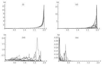
Figure 1: Bond yield spread between a digital bond (with all trajectories conditional on no default) and a sovereign bond. The bonds have maturity $T=2$ years. The a priori probability of default is taken to be $p_{0}=0.2$. We use (i) $\sigma_{2}=0.04$, (ii) $\sigma_{2}=0.2$, (iii) $\sigma_{2}=1$, and (iv) $\sigma_{2}=5$.

5 Credit-risky bonds with continuous market-
dependent recovery

Let us consider the case in which the credit-risky bond pays $H_{T}=X_{T}$ where $X_{T}$ is a discrete random variable which takes values $\{x_{0},x_{1},\ldots,x_{n}\}\in[0,1]$ with a priori probabilities $\{p_{0},p_{1},\ldots,p_{n}\}$, where $x_{n}>x_{n-1}>\ldots>x_{1}>x_{0}$. Such a payoff spectrum is a model for random recovery where at bond maturity one out of a discrete number of recovery levels may be realised. We can also consider credit-risky bonds with continuous random recovery in the event of default. In doing so, we introduce the notion of “market-dependent recovery”. Suppose that the payoff of the defaultable bond is given by

$$H_{T}=X_{T}+(1-X_{T})\,R(\xi_{TU}),$$ (5.1)

where $X_{T}$ takes the values $\{0,1\}$ with a priori probabilities $\{p_{0},p_{1}\}$. The recovery level $R:\mathbb{R}\rightarrow[0,1)$ is dependent on the information at time $T$ about the macroeconomic factor $X_{U}$. In this case, if the credit-risky bond defaults at maturity $T$, the recovery level of the bond depends on the state of the economy at time $U$ that is perceived in the market at time $T$. In other words, if the sentiment in the market at time $T$ is that the economy will have good times ahead, then a firm in a state of default at $T$ may have better chances to raise more capital from liquidation (or restructuring), thus increasing the level of recovery of the issued bond. We can price the cash flow (5.1) by applying equation (4), with $n=1,\,x_{0}=0$ and $x_{1}=1$. The result is:

$$B_{tT}=P_{tT}\pi_{1t}+\pi_{0t}\,\frac{1}{f(t,\xi_{tU})} \int_{-\infty}^{\infty}f\left(T,\nu_{tT}y+\frac{U-T}{U-t}\xi_{tU}\right)$$

$$\times R\left(\nu_{tT}y+\frac{U-T}{U-t}\xi_{tU}\right)\frac{1}{\sqrt{2\pi}}\exp{\left(-\mbox{$\textstyle\frac{1}{2}$}y^{2}\right)}\,\mbox{$\rm d$}y,$$ (5.2)

where $P_{tT}$ is given by equation (2.8). As an example, suppose that we choose the recovery function to be of the form $R(z)=1-\exp{(-z^{2})}.$ In this case, it is possible to have zero recovery when the value of the information process at time $t$ is $\xi_{tU}=-(U-t)/(U-T)\,\nu_{tT}Y$, thereby capturing the worst-case scenario in which bondholders lose their entire investment in the event of default.

The latter consideration is apt in the situation where the extent of recovery is determined by how difficult it is for the firm to raise capital by liquidating its assets, i.e. the exposure of the firm to the general economic environment. However, this model does not say much about how the quality of the management of the firm may influence recovery in the event of default. This observation brings us to another model of recovery. Default of a firm may be triggered by poor internal practices and (or) tough economic conditions. We now structure recovery by specifying the payoff of the credit risky bond by

$$H_{T}=X_{C}\left[X_{E}+(1-X_{E})R_{E}\right]+(1-X_{C})\left[X_{E}R_{C}+(1-X_{E})R_{CE}\right],$$ (5.3)

where $X_{C}$ and $X_{E}$ are random variables taking values in $\{0,1\}$ with a priori probabilities $\{p^{C}_{0},p^{C}_{1}\}$ and $\{p^{E}_{0},p^{E}_{1}\}$, respectively. We define $X_{C}$ and $X_{E}$ to be indicators of good management of the company and a strong economy, respectively. We set $R_{C}$ to be a continuous random variable assuming values in the interval $[0,1)$. We take $R_{E}$ to be a function of $\xi_{TU}$, and $R_{CE}$ to be a function of $\xi_{TU}$ and $R_{C}$, where both $R_{E}$ and $R_{CE}$ assume values in the interval $[0,1)$.

The payoff in equation (5.3) covers the following situations: First, we suppose that despite good overall management of the firm, default is triggered as a result of a depressed economy. Here, $X_{C}=1$ and $X_{E}=0$ which implies that $H_{T}=R_{E}$. Therefore the recovery is dependent on the state of the economy at time $T$ and thus, how difficult it has been for the firm to raise funds. It is also possible that a firm can default in otherwise favourable economic conditions, perhaps due to the management’s negligence. In this case we have $X_{E}=1$ and $X_{C}=0$. Thus $H_{T}=R_{C}$ and the amount recovered is dependent on the level of mismanagement of the firm. Finally we have the worst case in which a firm is poorly managed, $X_{C}=0$, and difficult economic times prevail, $X_{E}=0$. Recovery is given by the amount $H_{T}=R_{CE}$, which is dependent on both, the extent of mismanagement of the firm and how much capital the firm can raise in the face of an economic downturn. The particular payoff structure (5.3) is used in Macrina (2006) to model the dependence structure between two credit-risky discount bonds that share market factors in common. Further investigation may include the situation where one models such dependence structures for bonds subject to stochastic interest rates and featuring recovery functions of the form (5.3).

6 Call option price process

Let $\{C_{st}\}_{0\leq s\leq t<T}$ be the price process of a European-style call option with maturity $t$ and strike $K$, written on a defaultable bond with price process $\{B_{tT}\}$. The price of such an option at time $s$ is given by

$$C_{st}=\frac{1}{\pi_{s}}\,\mathbb{E}^{\mathbb{P}}\left[\pi_{t}\left(B_{tT}-K\right)^{+}|\,\mathcal{F}_{s}\right].$$ (6.1)

We recall that if the payoff of the credit-risky bond is $H_{T}=X_{T}$, then the price of the bond at time $t$ is

$$B_{tT}=P_{tT}\sum^{n}_{i=0}\pi_{it}\,x_{i},$$ (6.2)

where $P_{tT}$ is given by equation (2.8) and the conditional density $\pi_{it}$ is defined in equation (4.14). The filtration $\{\mathcal{F}_{t}\}$ is generated by the information processes $\{\xi_{tT}\}$ and $\{\xi_{tU}\}$, and the pricing kernel $\{\pi_{t}\}$ is of the form

$$\pi_{t}=M_{t}\,f(t,\xi_{tU}),$$ (6.3)

with $\{M_{t}\}$ satisfying equation (4.3). Then the price of the option at time $s$ is expressed by

$$C_{st}=\frac{1}{M_{s}\,f(s,\xi_{sU})}\,\mathbb{E}^{\mathbb{P}}\left[M_{t}\,f(t,\xi_{tU})\left(B_{tT}-K\right)^{+}\,|\,\xi_{sT},\xi_{sU}\right].$$ (6.4)

We recall that the two information processes are independent, and use the martingale $\{M_{t}\}$ to change the measure as follows:

$$C_{st}=\frac{1}{f(s,\xi_{sU})}\,\mathbb{E}^{\mathbb{B}_{U}}\left[f(t,\xi_{tU})\,\mathbb{E}^{\mathbb{P}}\left[\left(P_{tT}\sum^{n}_{i=0}\pi_{it}\,x_{i}-K\right)^{+}\bigg{|}\,\xi_{sT}\right]\bigg{|}\,\xi_{sU}\right].$$ (6.5)

We first simplify the inner conditional expectation by following an analogous calculation to that in Brody et al. (2007), Section 9. The difference is that the discount factor $\{P_{tT}\}$ in (6.5) is stochastic. However since $\{P_{tT}\}$ is driven by $\{\xi_{tU}\}$, it is unaffected by the conditioning of the inner expectation, allowing us to use the result in Brody et al. (2007). Let us introduce $\{\Phi_{t}\}$ by

$$\Phi_{t}=\sum^{n}_{i=0}p_{it},$$ (6.6)

where $p_{it}=p_{i}\exp{\left[\frac{T}{T-t}\left(\sigma_{2}x_{i}\,\xi_{tT}-\tfrac{1}{2}\,\sigma_{2}^{2}\,x_{i}^{2}\,t\right)\right]}$. We write the inner expectation as

$$\mathbb{E}^{\mathbb{P}}\left[\left(P_{tT}\sum^{n}_{i=0}\pi_{it}\,x_{i}-K\right)^{+}\bigg{|}\,\xi_{sT}\right]=\mathbb{E}^{\mathbb{P}}\left[\frac{1}{\Phi_{t}}\left(\sum^{n}_{i=0}\left(P_{tT}\,x_{i}-K\right)p_{it}\right)^{+}\bigg{|}\,\xi_{sT}\right].$$ (6.7)

The process $\{\Phi_{t}^{-1}\}$ induces a change of measure from $\mathbb{P}$ to the bridge measure $\mathbb{B}_{T}$, under which $\{\xi_{tT}\}$ is a Brownian bridge; this allows us to use Bayes formula to express the expectation as follows:

$$\mathbb{E}^{\mathbb{P}}\left[\frac{1}{\Phi_{t}}\left(\sum^{n}_{i=0}\left(P_{tT}\,x_{i}-K\right)p_{it}\right)^{+}\bigg{|}\,\xi_{sT}\right]$$

$$\hskip 156.49014pt=\frac{1}{\Phi_{s}}\mathbb{E}^{\mathbb{B}_{T}}\left[\left(\sum^{n}_{i=0}\left(P_{tT}\,x_{i}-K\right)p_{it}\right)^{+}\bigg{|}\,\xi_{sT}\right].$$ (6.8)

In order to compute the expectation we introduce the Gaussian random variable $Z_{st}$, defined by

$$Z_{st}=\frac{\xi_{tT}}{T-t}-\frac{\xi_{sT}}{T-s},$$ (6.9)

which is independent of $\{\xi_{uT}\}_{0\leq u\leq s}$. It is possible to find the critical value, for which the argument of the expectation vanishes, in closed form if it is assumed that the defaultable bond is binary. So, for $n=1$, the critical value $z^{\ast}$ is given by

$$z^{\ast}=\frac{\ln\left[\frac{\pi_{0s}(K-x_{0}P_{tT})}{\pi_{1s}(x_{1}P_{tT}-K)}\right]+\frac{1}{2}\sigma_{2}^{2}\left(x_{1}^{2}-x_{0}^{2}\right)\alpha_{st}^{2}\,T^{2}}{\sigma_{2}\,(x_{1}-x_{0})\,\alpha_{st}\,T},$$ (6.10)

where $\alpha_{st}^{2}=\textup{Var}^{\mathbb{B}_{T}}[Z_{st}]$. The computation of the expectation amounts to two Gaussian integrals reducing to cumulative normal distribution functions, which we denote by $N[x]$. We obtain the following:

$$\mathbb{E}^{\mathbb{P}}\left[\left(P_{tT}\sum^{1}_{i=0}\pi_{it}\,x_{i}-K\right)^{+}\bigg{|}\,\xi_{sT}\right]= \pi_{1s}(P_{tT}x_{1}-K)N[d^{+}_{s}]$$

$$-\pi_{0s}(K-P_{tT}x_{0})N[d^{-}_{s}],$$ (6.11)

where

$$d^{\pm}_{s}=\frac{\ln\left[\frac{\pi_{1s}(x_{1}P_{tT}-K)}{\pi_{0s}(K-x_{0}P_{tT})}\right]\pm\frac{1}{2}\sigma_{2}^{2}\left(x_{1}-x_{0}\right)^{2}\alpha_{st}^{2}\,T^{2}}{\sigma_{2}\,(x_{1}-x_{0})\,\alpha_{st}\,T}.$$ (6.12)

We can now insert this intermediate result into equation (6.5) for $n=1$; we have

$$C_{st}=\frac{1}{f(s,\xi_{sU})}\,\mathbb{E}^{\mathbb{B}_{U}}\left[f(t,\xi_{tU})\left[\pi_{1s}(P_{tT}x_{1}-K)N[d^{+}_{s}]\right.\right.$$

$$\hskip 156.49014pt\left.\left.-\pi_{0s}(K-P_{tT}x_{0})N[d^{-}_{s}]\right]|\,\xi_{sU}\right].$$ (6.13)

We emphasize that $\{P_{tT}\}$ is given by a function $P(t,T,\xi_{tU})$ and thus is affected by the conditioning with respect to $\xi_{sU}$. To compute the expectation in equation (6), we use the same technique as in Section 4 and introduce the Gaussian random variable $Y_{st}$, defined by

$$Y_{st}=\xi_{tU}-\frac{U-t}{U-s}\xi_{sU},$$ (6.14)

with mean zero and variance $\nu^{2}_{st}=\textrm{Var}^{\mathbb{B}_{U}}[Y_{st}]$. Thus, as shown in the previous sections, the outer conditional expectation reduces to a Gaussian integral:

$$C_{st}=\frac{1}{f(s,\xi_{sU})} \int_{-\infty}^{\infty}f\left(t,\nu_{st}y+\frac{U-t}{U-s}\,\xi_{sU}\right)\frac{1}{\sqrt{2\pi}}\exp\left(-\tfrac{1}{2}y^{2}\right)$$

$$\times\left[\pi_{1s}\left(P\left(t,T,\nu_{st}y+\frac{U-t}{U-s}\,\xi_{sU}\right)x_{1}-K\right)N[d^{+}_{s}(y)]\right.$$

$$\hskip 14.22636pt\left.-\pi_{0s}\left(K-P\left(t,T,\nu_{st}y+\frac{U-t}{U-s}\,\xi_{sU}\right)x_{0}\right)N[d^{-}_{s}(y)]\right]\,\mbox{$\rm d$}y.$$ (6.15)

Therefore we obtain a semi-analytical pricing formula for a call option on a defaultable bond in a stochastic interest rate setting. The integral in equation (6) can be evaluated using numerical methods once the function $f(t,x)$ is specified.

7 Hybrid securities

So far we have focused on the pricing of credit-risky bonds with stochastic discounting. The formalism presented in the above sections can also be applied to price other types of securities. In particular, as an example of a hybrid security, we show how to price an inflation-linked credit-risky discount bond. While such a security has inherent credit risk, it offers bondholders protection against inflation. This application also gives us the opportunity to extend the thus far presented pricing models to the case where $n$ independent information processes are employed. We shall call such models, “multi-dimensional pricing models”.

In what follows, we consider three independent information processes, $\{\xi_{tT}\}$, $\{\xi_{tU_{1}}\}$ and $\{\xi_{tU_{2}}\}$, defined by

$$\xi_{tT}=\sigma\,t\,X_{T}+\beta_{tT}, \xi_{tU_{1}}=\sigma_{1}\,t\,X_{U_{1}}+\beta_{tU_{1}}, \xi_{tU_{2}}=\sigma_{2}\,t\,X_{U_{2}}+\beta_{tU_{2}},$$ (7.1)

where $0\leq t\leq T<U_{1}\leq U_{2}$. The positive random variable $X_{T}$ is discrete, while $X_{U_{1}}$, $X_{U_{2}}$ are assumed to be continuous. The market filtration $\{\mathcal{F}_{t}\}$ is generated jointly by the three information processes. Let $\{C_{t}\}_{t\geq 0}$ be a price level process, e.g., the process of the consumer price index. The price $Q_{tT}$, at time $t$, of an inflation-linked discount bond that pays $C_{T}$ units of a currency at maturity $T$, is

$$Q_{tT}=\frac{\mathbb{E}^{\mathbb{P}}\left[\pi_{T}C_{T}|\,\mathcal{F}_{t}\right]}{\pi_{t}}.$$ (7.2)

We now make use of the “foreign exchange analogy” [see, e.g., Brigo & Mercurio (2006), Brody et al. (2008), Hinnerich (2008), Hughston (1998), Mercurio (2005)] in which the nominal pricing kernel $\{\pi_{t}\}$, and the real pricing kernel $\{\pi^{R}_{t}\}$, are viewed as being associated with “domestic” and “foreign” economies respectively, with the price level process $\{C_{t}\}$, acting as an “exchange rate”. The process $\{C_{t}\}$ is expressed by the following ratio:

$$C_{t}=\frac{\pi^{R}_{t}}{\pi_{t}}.$$ (7.3)

For further details about the modelling of the real and the nominal pricing kernels, and the pricing of inflation-linked assets, we refer to Hughston & Macrina (2009). In what follows, we make use of the method proposed in Hughston & Macrina (2009) to price an example of an inflation-linked credit-risky discount bond (ILCR) that, at maturity $T$, pays a cash flow $H_{T}=C_{T}H(X_{T},\xi_{TU_{1}},\xi_{TU_{2}})$. The price $H_{tT}$ at time $t\leq T$ of such a bond is

$$H_{tT}=\frac{1}{\pi_{t}}\mathbb{E}^{\mathbb{P}}\left[\pi^{R}_{T}\,H(X_{T},\xi_{TU_{1}},\xi_{TU_{2}})\,\big{|}\,\mathcal{F}_{t}\right],$$ (7.4)

where we have used relation (7.3). We choose to model the real and the nominal pricing kernels by

$$\pi_{t}=M^{(1)}_{t}M^{(2)}_{t}\,f(t,\xi_{tU_{1}},\xi_{tU_{2}}) \pi^{R}_{t}=M^{(1)}_{t}M^{(2)}_{t}\,g(t,\xi_{tU_{1}},\xi_{tU_{2}}),$$ and (7.5)

where $f(t,x,y)$ and $g(t,x,y)$ are two functions of three variables. The process $\{M^{(i)}_{t}\}_{0\leq t\leq T<U_{i}}$ for $i=1,2$ is a martingale that induces a change of measure to the bridge measure $\mathbb{B}_{i}$. We recall that the information process $\{\xi_{tU_{i}}\}$ has the law of a Brownian bridge under the measure $\mathbb{B}_{i}$. In order to work out the expectation in (7.4) with the pricing kernel models introduced in (7.5), we can also define a process $\{M_{t}\}$ by

$$M_{t}=M^{(1)}_{t}M^{(2)}_{t},$$ (7.6)

where $0\leq t\leq T<U_{1}\leq U_{2}$. Since the information processes $\{\xi_{tU_{1}}\}$ and $\{\xi_{tU_{2}}\}$ are independent, $\{M_{t}\}$ is itself an $(\{\mathcal{F}_{t}\},\mathbb{P})$-martingale, with $M_{0}=1$ and $\mathbb{E}^{\mathbb{P}}[M_{t}]=1$. Thus $\{M_{t}\}$ can be used to effect a change of measure from $\mathbb{P}$ to a bridge measure $\mathbb{B}$, under which the random variables $\xi_{tU_{1}}$ and $\xi_{tU_{2}}$ have the distribution of a Brownian bridge for $0\leq t\leq T<U_{1}$. This can be verified as follows: $\{\xi_{tU_{1}}\}$ is a Gaussian process with mean

$$\mathbb{E}^{\mathbb{B}}[\xi_{tU_{1}}]=\mathbb{E}^{\mathbb{B}_{1}}\left[\frac{M_{t}}{M_{t}^{(1)}}\xi_{tU_{1}}\right]=\mathbb{E}^{\mathbb{B}_{1}}\left[M^{(2)}_{t}\right]\,\mathbb{E}^{\mathbb{B}_{1}}[\xi_{tU_{1}}]=0,$$ (7.7)

due to the independence property of $\{\xi_{tU_{1}}\}$ and $\{\xi_{tU_{2}}\}$. Furthermore, for $0\leq s\leq t\leq T<U_{1}$, the covariance is given by

$$\mathbb{E}^{\mathbb{B}}[\xi_{sU_{1}}\xi_{tU_{1}}]=\mathbb{E}^{\mathbb{B}_{1}}\left[M^{(2)}_{t}\right]\,\mathbb{E}^{\mathbb{B}_{1}}[\xi_{sU_{1}}\xi_{tU_{1}}]=\mathbb{E}^{\mathbb{P}}[M_{t}]\,\mathbb{E}^{\mathbb{B}_{1}}[\xi_{sU_{1}}\xi_{tU_{1}}]=\frac{s(U_{1}-t)}{U_{1}}.$$ (7.8)

The same can be shown for $\{\xi_{tU_{2}}\}$.

By use of $\{M_{t}\}$ and the Bayes formula, and the fact that $\{\xi_{tT}\}$, $\{\xi_{tU_{1}}\}$ and $\{\xi_{tU_{2}}\}$ are $\{\mathcal{F}_{t}\}$-Markov processes, equation (7.4) reduces to

$$H_{tT}=$$

$$\frac{1}{f(t,\xi_{tU_{1}},\xi_{tU_{2}})}\mathbb{E}^{\mathbb{B}}\left[\mathbb{E}^{\mathbb{P}}\left[g(T,\xi_{TU_{1}},\xi_{TU_{2}})H\left(X_{T},\xi_{TU_{1}},\xi_{TU_{2}}\right)\,\big{|}\,\xi_{tT}\right]\big{|}\,\xi_{tU_{1}},\xi_{tU_{2}}\right].$$ (7.9)

Next we repeat an analogous calculation to the one leading from equation (4.8) to expression (4). For the ILCR discount bond under consideration, we obtain

$$H_{tT}=\frac{1}{f(t,\xi_{tU_{1}},\xi_{tU_{2}})}\sum^{n}_{i=0}\pi_{it}\int_{-\infty}^{\infty}\int_{-\infty}^{\infty} g\left(T,z(y_{1}),z(y_{2})\right)H\left(x_{i},z(y_{1}),z(y_{2})\right)$$

$$\times\tfrac{1}{2\pi}\,\exp\left[-\tfrac{1}{2}\left(y^{2}_{1}+y^{2}_{2}\right)\right]\,\mbox{$\rm d$}y_{1}\,\mbox{$\rm d$}y_{2}.$$ (7.10)

Here the conditional density $\pi_{it}$ is given by an expression analogous to the one in equation (4.14) and, $z(y_{k})$ is defined for $k=1,2$ by

$$z(y_{k})=\nu^{(k)}_{tT}\,y_{k}+\frac{U_{k}-T}{U_{k}-t}\,\xi_{tU_{k}},\quad\textrm{where}\quad\nu^{(k)}_{tT}=\sqrt{\frac{(T-t)(U_{k}-T)}{U_{k}-t}}.$$ (7.11)

In the special case where $H_{T}=X_{T}$, the expression for the price at time $t$ of the ILCR discount bond simplifies to

$$H_{tT}=Q_{tT}\sum^{n}_{i=0}\pi_{it}\,x_{i}.$$ (7.12)

Here $Q_{tT}$ is the price of an inflation-linked discount bond that depends on the information processes $\{\xi_{tU_{1}}\}$ and $\{\xi_{tU_{2}}\}$. In particular, a formula similar to (6) can be derived for the price of a European-style call option written on an ILCR bond with price process given by (7.12) with $n=1$. We note here that similar pricing formulae can be derived for credit-risky discount bonds traded in a foreign currency. In this case the real pricing kernel, and thus the real interest rate, is associated with the pricing kernel denominated in the foreign currency. On the other hand, the nominal pricing kernel is associated with the domestic currency, thus giving rise to the domestic interest rate.

8 Credit-risky coupon bonds

Let $\{T_{k}\}_{k=1,\ldots,n}$ be a collection of fixed dates where $0\leq t\leq T_{1}\leq\ldots\leq T_{n}$. We consider the valuation of a credit-risky bond with coupon payment $H_{T_{k}}$ at time $T_{k}$ and maturity $T_{n}$. The bond is in a state of default as soon as the first coupon payment does not occur. We denote the price process of the coupon bond by $\{B_{tT_{n}}\}$ and introduce $n$ independent random variables $X_{T_{1}},\ldots,X_{T_{n}}$ that are applied to construct the cash flows $H_{T_{k}}$ given by

$$H_{T_{k}}=\mathbf{c}\prod^{k}_{j=1}X_{T_{j}},$$ (8.1)

for $k=1,\ldots,n-1$, and for $k=n$ by

$$H_{T_{n}}=\mathbf{(c+p)}\prod^{n}_{j=1}X_{T_{j}}.$$ (8.2)

Here $\mathbf{c}$ and $\mathbf{p}$ denote the coupon and principal payment, respectively, and the random variables $\{X_{T_{k}}\}_{k=1,\ldots,n}$ take values in $\{0,1\}$. With each factor $X_{T_{k}}$ we associate an information process $\{\xi_{tT_{k}}\}$ defined by

$$\xi_{tT_{k}}=\sigma_{k}\,t\,X_{T_{k}}+\beta_{tT_{k}}.$$ (8.3)

Furthermore we introduce another information process $\{\xi_{tU}\}$ given by

$$\xi_{tU}=\sigma\,t\,X_{U}+\beta_{tU}\qquad(0\leq t\leq T_{n}<U)$$ (8.4)

that we reserve for the modelling of the pricing kernel. The market filtration $\{\mathcal{F}_{t}\}$ is generated jointly by the $n+1$ information processes, that is $\{\xi_{tT_{k}}\}_{k=1,\ldots,n}$ and $\{\xi_{tU}\}$. Following the method in Section 4, we model the pricing kernel $\{\pi_{t}\}$ by

$$\pi_{t}=M_{t}\,f(t,\xi_{tU}),$$ (8.5)

where the density martingale $\{M_{t}\}$ which induces a change of measure to the bridge measure satisfies equation (2.3). Armed with these ingredients we are now in the position to write down the formula for the price $B_{tT_{n}}$ at time $t$ of the credit-risky coupon bond:

$$B_{tT_{n}} =\frac{1}{\pi_{t}}\sum^{n}_{k=1}\,\mathbb{E}^{\mathbb{P}}\left[\pi_{T_{k}}\,H_{T_{k}}\,\big{|}\,\xi_{tT_{1}},\ldots,\xi_{tT_{k}},\xi_{tU}\right],$$ (8.6)

$$=\frac{1}{M_{t}\,f(t,\xi_{tU})}\sum^{n}_{k=1}\,\mathbb{E}^{\mathbb{P}}\left[M_{T_{k}}\,f(T_{k},\xi_{T_{k}U})\,\mathbf{c}\prod^{k}_{j=1}X_{T_{j}}\,\bigg{|}\,\xi_{tT_{1}},\ldots,\xi_{tT_{k}},\xi_{tU}\right]$$

$$\indent+\frac{1}{M_{t}\,f(t,\xi_{tU})}\,\mathbb{E}^{\mathbb{P}}\left[M_{T_{n}}\,f(T_{n},\xi_{T_{n}U})\,\mathbf{p}\prod^{n}_{j=1}X_{T_{j}}\,\bigg{|}\,\xi_{tT_{1}},\ldots,\xi_{tT_{n}},\xi_{tU}\right].$$

To compute the expectation, we use the approach presented in Section 4. Since the pricing kernel and the cash flow random variables $H_{T_{k}}$, $k=1,\ldots,n$, are independent, we conclude that the expression for the bond price $B_{tT_{n}}$ simplifies to

$$B_{tT_{n}}=\mathbf{c}\,\sum^{n}_{k=1}P_{tT_{k}} \mathbb{E}^{\mathbb{P}}\left[\prod^{k}_{j=1}X_{T_{j}}\,\bigg{|}\,\xi_{tT_{1}},\ldots,\xi_{tT_{k}}\right]$$

$$+\mathbf{p}\,P_{tT_{n}}\mathbb{E}^{\mathbb{P}}\left[\prod^{n}_{j=1}X_{T_{j}}\,\bigg{|}\,\xi_{tT_{1}},\ldots,\xi_{tT_{n}}\right],$$ (8.7)

where the discount bond system $\{P_{tT_{k}}\}$ is given by

$$P_{tT_{k}}=\frac{1}{f(t,\xi_{tU})}\int_{-\infty}^{\infty}f\left(T_{k},\nu_{tT_{k}}y_{k}+\frac{U-T_{k}}{U-t}\,\xi_{tU}\right)\frac{1}{\sqrt{2\pi}}\exp\left(-\tfrac{1}{2}y_{k}^{2}\right)\mbox{$\rm d$}y_{k},$$ (8.8)

and $\nu^{2}_{tT_{k}}=(T_{k}-t)(U-T_{k})/(U-t)$. We note that formula (8.6) can be simplified further since the expectations therein can be worked out explicitly due to the independence property of the information processes. We have,

$$\mathbb{E}^{\mathbb{P}}\left[\prod^{k}_{j=1}X_{T_{j}}\,\bigg{|}\,\xi_{tT_{1}},\ldots,\xi_{tT_{k}}\right]=\prod^{k}_{j=1}\pi_{1t}^{(j)},$$ (8.9)

where the conditional density $\pi_{1t}^{(j)}$ at time $t$ that the random variable $X_{T_{j}}$ takes value one is given by

$$\pi^{(j)}_{1t}=\frac{p^{(j)}_{1}\exp{\left[\frac{T_{j}}{T_{j}-t}\left(\sigma_{j}\,\xi_{tT_{j}}-\mbox{$\textstyle\frac{1}{2}$}\sigma_{j}^{2}t\right)\right]}}{p^{(j)}_{0}+p^{(j)}_{1}\exp{\left[\frac{T_{j}}{T_{j}-t}\left(\sigma_{j}\,\xi_{tT_{j}}-\mbox{$\textstyle\frac{1}{2}$}\sigma_{j}^{2}t\right)\right]}}.$$ (8.10)

Here $p^{(j)}_{1}=\mathbb{P}[X_{T_{j}}=1]$. Thus, the price $B_{tT_{n}}$ at time $t$ of the credit-risky coupon bond is given by

$$B_{tT_{n}}=\sum_{k=1}^{n}\mathbf{c}\,P_{tT_{k}}\prod_{j=1}^{k}\pi_{1t}^{(j)}+\mathbf{p}\,P_{tT_{n}}\prod_{j=1}^{n}\pi^{(j)}_{1t}.$$ (8.11)

At this stage, we observe that the price of a credit-risky coupon bond has been derived for the case in which the cash flow functions $H_{T_{k}},\;k=1,\ldots,n,$ do not depend on the information available at time $T_{k}$ about the macroeconomic factor $X_{U}$, thereby leading to independence between the discount bond system and the credit-risky component of the bond. This is generalized in a straightforward manner by considering cash flow functions of the form

$$H_{T_{k}}=H(X_{T_{1}},\ldots,X_{T_{k}},\xi_{T_{k}U}),$$ (8.12)

for $k=1,\ldots,n$. The valuation of such cash flows at time $t$ may include the case treated in (4), however endowed with coupon payments.

As an illustration we consider the situation in which the bond pays a coupon $\mathbf{c}$ at $T_{k},\;k=1,\ldots,n,$ and the principal amount $\mathbf{p}$ at $T_{n}$. Upon default, market-dependent recovery given by $R_{k}(\xi_{T_{k}U})$ (as a percentage of coupon plus principal) is paid at $T_{k}$. For simplicity, we consider $n=2$. In this case, the random cash flows of the bond are given by

$$H_{T_{1}} =\mathbf{c}X_{T_{1}}+\mathbf{(c+p)}\,R_{1}(\xi_{T_{1}U})(1-X_{T_{1}}),$$

$$H_{T_{2}} =\mathbf{(c+p)}\,X_{T_{1}}\left[X_{T_{2}}+R_{2}(\xi_{T_{2}U})(1-X_{T_{2}})\right].$$

By making use of the technique presented in Section 5, we can express the price of the credit-risky coupon bond by

$$B_{tT_{2}} =\mathbf{c}\,P_{tT_{1}}\pi^{(1)}_{1t}+\mathbf{(c+p)}\,P_{tT_{2}}\pi^{(1)}_{1t}\pi^{(2)}_{1t}$$

$$+\mathbf{(c+p)}\left[\pi^{(1)}_{0\,t}\frac{1}{f(t,\xi_{tU})}\int_{-\infty}^{\infty}f\left(T_{1},m(y_{1})\right)\,R_{1}\left(m(y_{1})\right)\frac{1}{\sqrt{2\pi}}\exp{\left(-\tfrac{1}{2}y^{2}_{1}\right)}\,\mbox{$\rm d$}y_{1}\right.$$

$$\hskip 14.22636pt\left.+\pi^{(1)}_{1t}\pi^{(2)}_{0\,t}\frac{1}{f(t,\xi_{tU})}\int_{-\infty}^{\infty}f\left(T_{2},m(y_{2})\right)\,R_{2}\left(m(y_{2})\right)\frac{1}{\sqrt{2\pi}}\exp{\left(-\tfrac{1}{2}y^{2}_{2}\right)}\,\mbox{$\rm d$}y_{2}\right],$$

where, for $k=1,2$, we define

$$m(y_{k})=\nu_{tT_{k}}\,y_{k}+\frac{U-T_{k}}{U-t}\,\xi_{tU},\quad\quad\nu_{tT_{k}}=\sqrt{\frac{(T_{k}-t)(U-T_{k})}{U-t}}.$$ (8.13)

9 Credit-sensitive pricing kernels

We fix the dates $T_{1}$ and $T_{2}$, where $T_{1}\leq T_{2}$, to which we associate the economic factors $X_{T_{1}}$ and $X_{T_{2}}$ respectively. The first factor is identified with a debt payment at time $T_{1}$. For example $X_{T_{1}}$ could be a coupon payment that a country is obliged to make at time $T_{1}$. The second factor, $X_{T_{2}}$, could be identified with the measured growth (possibly negative) in the employment level in the same country at time $T_{2}$ since the last published figure. In such an economy, with two random factors only, it is plausible that the prices of the treasuries fluctuate according to the noisy information market participants will have about the outcome of $X_{T_{1}}$ and $X_{T_{2}}$. Thus the price of a sovereign bond with maturity $T$, where $0\leq t\leq T<T_{1}\leq T_{2}$, is given by:

$$P_{tT}=\frac{1}{f(t,\xi_{tT_{1}},\xi_{tT_{2}})}\int^{\infty}_{-\infty}\int^{\infty}_{-\infty} f\left(T,\nu^{(1)}_{tT}y_{1}+\frac{T_{1}-T}{T_{1}-t}\xi_{tT_{1}},\nu^{(2)}_{tT}y_{2}+\frac{T_{2}-T}{T_{2}-t}\xi_{tT_{2}}\right)$$

$$\times\frac{1}{2\pi}\exp\left[-\tfrac{1}{2}\left(y^{2}_{1}+y^{2}_{2}\right)\right]\,\mbox{$\rm d$}y_{2}\,\mbox{$\rm d$}y_{1}.$$ (9.1)

In particular, the resulting interest rate process in this model is subject to the information processes $\{\xi_{tT_{1}}\}$ and $\{\xi_{tT_{2}}\}$ making it fluctuate according to information (both genuine and misleading) about the economy’s factors $X_{T_{1}}$ and $X_{T_{2}}$.

We now ask the following question: What type of model should one consider if the goal is to model a pricing kernel that is sensitive to an accumulation of losses? Or in other words, how should one model the nominal short rate of interest and the market price of risk processes if both react to the amount of debt accumulated by a country over a finite period of time?

To treat this question we need to introduce a model for an accumulation process. We shall adopt the method developed in Brody et al. (2008b), where the idea of a gamma bridge information process is introduced. It turns out that the use of such a cumulative process is suitable to provide an answer to the question above. In fact, if in the example above, the factor $X_{T_{1}}$ is identified with the total accumulated debt at time $T_{1}$, then the gamma bridge information process $\{\xi^{\gamma}_{tT_{1}}\}$, defined by

$$\xi^{\gamma}_{tT_{1}}=X_{T_{1}}\,\gamma_{tT_{1}}$$ (9.2)

where $\{\gamma_{tT_{1}}\}_{0\leq t\leq T_{1}}$ is a gamma bridge process that is independent of $X_{T_{1}}$, measures the level of the accumulated debt as of time $t$, $0\leq t\leq T_{1}$. If the market filtration is generated, among other information processes, also by the debt accumulation process, then asset prices that are calculated by use of this filtration, will fluctuate according to the updated information about the level of the accumulated debt of a country. We now work out the price of a sovereign bond for which the price process reacts both to Brownian and gamma information.

We consider the time line $0\leq t\leq T<T_{1}\leq T_{2}<\infty$. Time $T$ is the maturity date of a sovereign bond with unit payoff and price process $\{P_{tT}\}_{0\leq t\leq T}$. With the date $T_{1}$ we associate the factor $X_{T_{1}}$ and with the date $T_{2}$ the factor $X_{T_{2}}$. The positive random variable $X_{T_{1}}$ is independent of $X_{T_{2}}$, and both may be discrete or continuous random variables. Then we introduce the following information processes:

$$\xi^{\gamma}_{tT_{1}}=X_{T_{1}}\,\gamma_{tT_{1}}, \xi_{tT_{2}}=\sigma\,t\,X_{T_{2}}+\beta_{tT_{2}}.$$ (9.3)

The process $\{\xi^{\gamma}_{tT_{1}}\}$ is a gamma bridge information process, and it is taken to be independent of $\{\xi_{tT_{2}}\}$. The properties of the gamma bridge process $\{\gamma_{tT_{1}}\}$ are described in great detail in Brody et al. (2008b). We assume that the market filtration $\{\mathcal{F}_{t}\}_{t\geq 0}$ is generated jointly by $\{\xi^{\gamma}_{tT_{1}}\}$ and $\{\xi_{tT_{2}}\}$.

In this setting, the pricing kernel reacts to the updated information about the level of accumulated debt and, for the sake of example, also to noisy information about the likely level of employment growth at $T_{2}$. Thus we propose the following model for the pricing kernel:

$$\pi_{t}=M_{t}\,f\left(t,\xi^{\gamma}_{tT_{1}},\xi_{tT_{2}}\right)$$ (9.4)

where the process $\{M_{t}\}$ is the change-of-measure martingale from the probability measure $\mathbb{P}$ to the Brownian bridge measure $\mathbb{B}$, satisfying

$$\mbox{$\rm d$}M_{t}=-\,\sigma\frac{T_{2}}{T_{2}-t}\,\mathbb{E}\left[X_{T_{2}}\,|\,\xi_{tT_{2}}\right]M_{t}\,\mbox{$\rm d$}W_{t}.$$ (9.5)

Here $\{W_{t}\}$ is an $(\{\mathcal{F}_{t}\},\mathbb{P})$-Brownian motion. The formula for the price of the sovereign bond is given by

$$P_{tT}=\frac{\mathbb{E}^{\mathbb{P}}\left[M_{T}f\left(T,\xi^{\gamma}_{TT_{1}},\xi_{TT_{2}}\right)\big{|}\,\xi^{\gamma}_{tT_{1}},\xi_{tT_{2}}\right]}{M_{t}\,f\left(t,\xi^{\gamma}_{tT_{1}},\xi_{tT_{2}}\right)}.$$ (9.6)

We make use of the Markov property and the independence property of the information processes, together with the change of measure to express the bond price by

$$P_{tT}=\frac{\mathbb{E}^{\mathbb{P}}_{\gamma}\left[\mathbb{E}^{\mathbb{B}}\left[f\left(T,\xi^{\gamma}_{TT_{1}},\xi_{TT_{2}}\right)\big{|}\,\xi_{tT_{2}}\right]\big{|}\,\xi^{\gamma}_{tT_{1}}\right]}{f\left(t,\xi^{\gamma}_{tT_{1}},\xi_{tT_{2}}\right)}.$$ (9.7)

Here, the expectations $\mathbb{E}^{\mathbb{P}}_{\gamma}$ and $\mathbb{E}^{\mathbb{B}}$ are operators that apply according to the dependence of their argument on the random variables $\xi^{\gamma}_{TT_{1}}$ and $\xi_{TT_{2}}$ respectively. This is a direct consequence of the independence of $\{\xi^{\gamma}_{tT_{1}}\}$ and $\{\xi_{tT_{2}}\}$. We now use the technique adopted in the preceding sections, where we introduce the Gaussian random variable $Y_{tT}$ with mean zero and variance $\nu^{2}_{tT}=(T-t)(T_{2}-T)/(T_{2}-t),$ and the standard Gaussian random variable $Y$. By following the approach taken in Section 4, we can compute the inner expectation explicitly since the conditional expectation reduces to a Gaussian integral over the range of the random variable $Y$. Thus we obtain:

$$P_{tT}=\int^{\infty}_{-\infty}\frac{\mathbb{E}^{\mathbb{P}}_{\gamma}\left[f\left(T,\xi^{\gamma}_{TT_{1}},\nu_{tT}y+\frac{T_{2}-T}{T_{2}-t}\xi_{tT_{2}}\right)\,\big{|}\,\xi^{\gamma}_{tT_{1}}\right]}{f\left(t,\xi^{\gamma}_{tT_{1}},\xi_{tT_{2}}\right)}\,\frac{1}{\sqrt{2\pi}}\exp\left(-\tfrac{1}{2}y^{2}\right)\,\mbox{$\rm d$}y.$$ (9.8)

The feature of this model which sets it apart from those considered in preceding sections, is the fact that we have to calculate a gamma expectation $\mathbb{E}^{\mathbb{P}}_{\gamma}$. In this case, we cannot adopt the “usual” change-of-measure method we have used thus far. To this end we refer to the work in Brody et al. (2008b), where the price process of the Arrow-Debreu security for the case that it is driven by a gamma bridge information process is derived. We use this result and obtain for the Arrow-Debreu density process $\{A_{tT}\}$ the following expression:

$$A_{tT}(y_{\gamma})={\mathbb{E}}^{\mathbb{P}}\left[\delta(\xi^{\gamma}_{TT_{1}}-y_{\gamma})\,\big{|}\,\xi^{\gamma}_{tT_{1}}\right]$$ (9.9)

$$=\frac{{1\textup{{l}}}{\{y_{\gamma}>\xi^{\gamma}_{tT_{1}}\}}\,(y_{\gamma}-\xi^{\gamma}_{tT_{1}})^{m(T-t)-1}}{B[m(T-t),m(T_{1}-T)]}\frac{\int^{\infty}_{y_{\gamma}}p(x)\,x^{1-mT_{1}}(x-y_{\gamma})^{m(T_{1}-T)-1}\mbox{$\rm d$}x}{\int^{\infty}_{\xi^{\gamma}_{tT_{1}}}p(z)\,z^{1-mT_{1}}(z-\xi^{\gamma}_{tT_{1}})^{m(T_{1}-t)-1}\mbox{$\rm d$}z},$$ (9.10)

where $\delta(y)$ is the Dirac distribution and $p(x)$ is the a priori probability density of $X_{T_{1}}$. Here $B[a,b]$ is the beta function. Following Macrina (2006), Section 3.4, we consider a function $h(\xi^{\gamma}_{TT_{1}})$ of the random variable $\xi^{\gamma}_{TT_{1}}$ and note that for a suitable function $h$ we may write:

$$\mathbb{E}^{\mathbb{P}}_{\gamma}\left[h\left(\xi^{\gamma}_{TT_{1}}\right)\,\big{|}\,\xi^{\gamma}_{tT_{1}}\right]=\int^{\infty}_{-\infty}\mathbb{E}^{\mathbb{P}}_{\gamma}\left[\delta\left(\xi^{\gamma}_{TT_{1}}-y_{\gamma}\right)\big{|}\,\xi^{\gamma}_{tT_{1}}\right]h(y_{\gamma})\,\mbox{$\rm d$}y_{\gamma}.$$ (9.11)

Next we see that the conditional expectation under the integral is the Arrow-Debreu density (9.9) for which there is the closed-form expression (9.10). We go back to equation (9.8) and observe that the conditional expectation under the integral is of the form $\mathbb{E}^{\mathbb{P}}_{\gamma}\left[h\left(\xi^{\gamma}_{TT_{1}}\right)\big{|}\xi^{\gamma}_{tT_{1}}\right]$. Thus we can use (9.11) to calculate the gamma expectation in (9.8). We write:

$$\mathbb{E}^{\mathbb{P}}_{\gamma}\left[f\left(T,\xi^{\gamma}_{TT_{1}},\nu_{tT}\,y+\frac{T_{2}-T}{T_{2}-t}\,\xi_{tT_{2}}\right)\Big{|}\,\xi^{\gamma}_{tT_{1}}\right]$$

$$\hskip 85.35826pt=\int^{\infty}_{-\infty}A_{tT}\left(y_{\gamma}\right)f\left(T,y_{\gamma},\nu_{tT}\,y+\frac{T_{2}-T}{T_{2}-t}\,\xi_{tT_{2}}\right)\mbox{$\rm d$}y_{\gamma}.$$ (9.12)

We are now in the position to write down the bond price (9.8) in explicit form by using equation (9). We thus obtain:

$$P_{tT}=\int^{\infty}_{-\infty}\int^{\infty}_{-\infty}\,\frac{A_{tT}\left(y_{\gamma}\right)f\left(T,y_{\gamma},\nu_{tT}\,y+\frac{T_{2}-T}{T_{2}-t}\,\xi_{tT_{2}}\right)}{f\left(t,\xi^{\gamma}_{tT_{1}},\xi_{tT_{2}}\right)}\,\frac{1}{\sqrt{2\pi}}\exp\left(-\tfrac{1}{2}y^{2}\right)\mbox{$\rm d$}y_{\gamma}\,\mbox{$\rm d$}y.$$ (9.13)

The bond price can be written more concisely by defining

$$\tilde{f}\left(T,t,\xi^{\gamma}_{tT_{1}},\xi_{tT_{2}}\right)=\int^{\infty}_{-\infty}\int^{\infty}_{-\infty}\, A_{tT}\left(y_{\gamma}\right)f\left(T,y_{\gamma},\nu_{tT}y+\frac{T_{2}-T}{T_{2}-t}\,\xi_{tT_{2}}\right)$$

$$\times\frac{1}{\sqrt{2\pi}}\exp\left(-\tfrac{1}{2}\,y^{2}\right)\mbox{$\rm d$}y_{\gamma}\,\mbox{$\rm d$}y.$$ (9.14)

We thus have:

$$P_{tT}=\frac{\tilde{f}\left(T,t,\xi^{\gamma}_{tT_{1}},\xi_{tT_{2}}\right)}{f\left(t,\xi^{\gamma}_{tT_{1}},\xi_{tT_{2}}\right)}.$$ (9.15)

Future investigation in this line of research incorporates the constructions of processes $\{f(t,\xi^{\gamma}_{tT_{1}},\xi_{tT_{2}})\}$ such that the resulting pricing kernel (9.4) is an $(\{\mathcal{F}_{t}\},\mathbb{P})$-supermartingale. The appropriate choice of $f(t,x,y)$ depends also on a suitable description of the economic interplay of the information flows modelled by $\{\xi^{\gamma}_{tT_{1}}\}$ and $\{\xi_{tT_{2}}\}$. One might begin with looking at the situation in which the price of the bond depreciates due to a rising debt level and a higher level of employment. We conclude by observing that the gamma bridge information process may also be considered for the modelling of credit-risky bonds, where default is triggered by the firm’s accumulated debt exceeding a specified threshold at bond maturity. Random recovery models may be constructed using the technique in Section 5.

References

1. Akahori, J., Hishida, Y., Teichmann, J. and Tsuchiya, T. (2009),“A Heat Kernel Approach to Interest Rate Models”, arXiv:0910.5033.

2. Akahori, J. and Macrina, A. (2010), “Heat Kernel Interest Rate Models with Time-Inhomogeneous Markov Processes”, Ritsumeikan University, King’s College London and Kyoto University working paper.

3. Bielecki, T. R. and Rutkowski, M. (2002), Credit Risk: Modelling, Valuation and Hedging, Springer-Verlag, Berlin.

4. Brigo, D. and Mercurio, F. (2006), Interest Rate Models: Theory and Practice (with Smile, Inflation and Credit), Springer-Verlag, Berlin.

5. Brody, D. C., Crosby, J. and Li, H. (2008), “Convexity Adjustments in Inflation-Linked Derivatives”, Risk Magazine, September issue, 124-129.

6. Brody, D. C., Davis, M. H. A., Friedman, R. L. and Hughston, L. P. (2009), “Informed Traders”, Proceedings of the Royal Society London, A465, 1103–1122.

7. Brody, D. C., Hughston, L. P. and Macrina, A. (2007), “Beyond Hazard Rates: A New Framework to Credit Risk Modelling”, in Advances in Mathematical Finance, Festschrift Volume in Honour of Dilip Madan (eds Elliott R., Fu, M., Jarrow, R. and Yen, J. Y.), Birkhäuser, Basel.

8. Brody, D. C., Hughston, L. P. and Macrina, A. (2008a), “Information-Based Asset Pricing”, International Journal of Theoretical and Applied Finance, 11, 107–142.

9. Brody, D. C., Hughston, L. P. and Macrina, A. (2008b), “Dam Rain and Cumulative Gain”, Proceedings of the Royal Society London, A464, 1801–1822.

10. Flesaker, B. and Hughston, L. P. (1996), “Positive Interest”, Risk, 9, 46–49.

11. Hinnerich, M. (2008), “Inflation-Indexed Swaps and Swaptions”, Journal of Banking and Finance, 32, 2293–2306.

12. Hoyle, E., Hughston, L. P. and Macrina, A. (2009), “Lévy Random Bridges and the Modelling of Financial Information”, arXiv:0912.3652.

13. Hughston, L. P. (1998), “Inflation Derivatives”, Merrill Lynch and King’s College London working paper, with added note (2004).

14. Hughston, L. P. and Macrina, A. (2009), “Pricing Fixed-Income Securities in an Information-Based Framework”, arXiv:0911.1610.

15. Hunt, P. J. and Kennedy, J. E. (2004), Financial Derivatives in Theory and Practice, Wiley, Chichester.

16. Macrina, A. (2006), “An Information-Based Framework for Asset Pricing: $X$-factor Theory and its Applications”, PhD thesis, King’s College London.

17. Mercurio, F. (2005), “Pricing Inflation-Indexed Derivatives”, Quantitative Finance, 5, No. 3, 289-302.

18. Rogers, L. C. G. (1997), “The Potential Approach to the Term Structure of Interest Rates and Foreign Exchange Rates”, Mathematical Finance, 7, 157–176.

19. Rutkowski, M. and Yu, N. (2007), “An Extension of the Brody-Hughston-Macrina Approach to Modelling of Defaultable Bonds”, International Journal of Theoretical and Applied Finance, 10, 557–589.