Combinatorics of 1-particle irreducible $n$-point functions via coalgebra in quantum field theory

Abstract

We give a coalgebra structure on 1-vertex irreducible graphs which is that of a cocommutative coassociative graded connected coalgebra. We generalize the coproduct to the algebraic representation of graphs so as to express a bare 1-particle irreducible $n$-point function in terms of its loop order contributions. The algebraic representation is so that graphs can be evaluated as Feynman graphs.

I Introduction

In perturbative quantum field theory the $n$-point functions are given by weighted sums over all Feynman graphs of a given type. Each Feynman graph represents an integral which is often divergent. This is due to the fact that products of Feynman propagators with coincident spacetime points are not defined. In particular, all divergences of a given Feynman graph reside in the 1-particle irreducible (1PI) subgraphs. Therefore, these are essential for renormalization for it is enough to renormalize the 1PI graphs. The systematic generation of all (bare) 1PI Feynman graphs is traditionally dealt with via the Legendre transform of the generating functional of connected Green functions and iteration of the 1PI Dyson-Schwinger equations. Though this is the standard procedure, any method to straightforwardly manipulate 1PI Feynman graphs may actually be used. Here, we focus on the algorithm to generate all 1PI (i.e., 2-edge connected) graphs given in Ref. Me:biconn, . This is so that larger 1PI graphs are produced from smaller ones by increasing the number of their building blocks, the maximal 1-vertex irreducible (1VI) (i.e., biconnected) subgraphs. The decomposition of 1PI graphs in terms of their 1VI components is of interest to perturbative quantum field theory for the counterterm of a 1PI graph is given by the product of the counterterms of its 1VI components KS-F:critical .

The present work is closely related to Ref. MeOe:npoint, ; MeOe:loop, where recursion formulas to generate all trees and all connected graphs are given. The underlying structure is an algebraic representation of graphs based on the Hopf algebra structure of the symmetric algebra on monomials of time-ordered field operators given in Ref. BrOe:scalar, ; Br:meets, . This allowed to derive simple algebraic relations between complete, connected and 1PI $n$-point functions MeOe:npoint , and to express a connected $n$-point function in terms of its loop order contributions MeOe:loop . Here, we extend the latter result to 1PI $n$-point functions. To this end, we give a coalgebra structure on 1VI Feynman graphs which is that of a cocommutative coassociative graded connected coalgebra. We generalize the coproduct to a map on the algebraic representation whose action is analogous to that of the coproduct. We use the truncated coproduct MeOe:npoint and the analog of the coproduct on 1VI graphs to derive algebraic expressions of the recursion formulas to generate all 1VI and all 1PI graphs given in Ref. Me:biconn, . As in Ref. MeOe:npoint, ; MeOe:loop, , the underlying algorithms are amenable to direct implementation and allow efficient calculations of graphs as well as their values as Feynman graphs. Moreover, all results apply both to bosonic and fermionic fields. Note, however, that no type of renormalization procedure is taken into account. In this sense the computed $n$-point functions may be considered as bare ones.

This paper is organized as follows: Section II.1 recalls the definition of Feynman graphs and their relation to the $n$-point functions. Section II.2 reviews the Hopf algebra structure of the associative algebra on monomials of time-ordered field operators given in Ref. BrOe:scalar, ; Br:meets, . Section III recalls the Hopf algebraic representation of graphs given in Ref. MeOe:npoint, ; MeOe:loop, and gives a non-associative graph multiplication. Section IV gives a coalgebra structure on 1VI Feynman graphs and generalizes the coproduct to the algebraic representation. Section V gives the basic linear maps to construct 1VI or 1PI graphs. Sections VI.1 and VI.2 express the recursion formulas to generate 1VI and 1PI graphs given in Ref. Me:biconn, in a completely algebraic language, while Section VI.3 deals with their interpretation in terms of the 1PI $n$-point functions.

II Basics

In the following we are concerned with a generic perturbative quantum field theory with fields $\phi(x)$ as operator valued distributions with adequate test functions. Here, $x$ represents a label that specifies spacetime coordinates, particle type, Minkowski indices, spin, colour, etc. The elementary field operators are local fields whose propagation and interactions may be described by local Hamiltonian or Lagrangian densities. For more information on these, we refer the reader to any standard textbook on quantum field theory such as Ref. ItZu:qft, . Note, however, that the essential property used in this paper is that they are (labeled) elements of a vector space. Moreover, as in Ref. MeOe:npoint, ; MeOe:loop, , for simplicity we limit ourselves in the following exposition to a purely bosonic theory with a single scalar field. A more extensive discussion including fermionic fields is given in Section VI D of Ref. MeOe:npoint, .

II.1 Feynman graphs

We review the essentials about Feynman graphs that can be found in any textbook on quantum field theory such as Ref. ItZu:qft, .

The following notation will be used in all the paper: by $\gamma$, we denote a (vertex) numbered graph while by $\bar{\gamma}$, we denote the associated Feynman graph.

In perturbative quantum field theory, the calculation of physical quantities consists of evaluating integrals represented by Feynman graphs. These are graphs that carry certain labels on vertices and edges. The former correspond to the interaction terms of the Lagrangian, while the latter may correspond to momenta and internal indices (usually indicated by different styles of lines, e.g., straight for fermions, wiggly for bosons, etc). Here, we assume that labels are attached to the free ends of external edges, so that internal labels shall be summed or integrated over.

The simplest Feynman graph is the graph consisting of an external edge only, its two end points labeled $x_{1}$ and $x_{2}$, respectively, and its value corresponding to the Feynman propagator $G_{F}(x_{1},x_{2})$, see Figure 1 (a). The latter is a Green’s function for the free Klein-Gordon equation which is interpreted as the probability amplitude that a particle changes position or some other attribute. The Feynman propagator is invertible under convolution. Its inverse $G_{F}^{-1}$ is determined by the following equation:

$$\int\mathrm{d}y\,G_{F}(x,y)G_{F}^{-1}(y,z)=\delta(x,z)\,.$$ (1)

Besides changing spacetime positions or other properties, a particle can split into many other particles. The probability amplitude that this happens is represented by (bare) interacting vertices. The value of a graph that consists of a vertex with external edges labeled $x_{1},\dots,x_{n}$, is given by the $n$-point vertex function $\mathscr{V}^{(n)}(x_{1},\dots,x_{n})$:

$$\mathscr{V}^{(n)}(x_{1},\ldots,x_{n}):=\int\mathrm{d}y_{1}\ldots\mathrm{d}y_{n}\,\Sigma^{(n)}(y_{1},\ldots,y_{n})G_{F}(x_{1},y_{1})\ldots G_{F}(x_{n},y_{n})\,,$$ (2)

where $\Sigma^{(n)}$ denotes the truncated $n$-point vertex function.

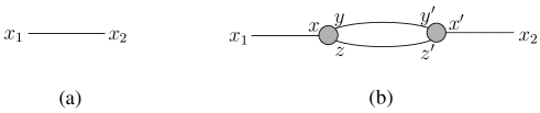
Figure 1: Examples of Feynman graphs. (a) The Feynman propagator; (b) A contribution to a interaction of the fields $\phi(x_{1})$ and $\phi(x_{2})$.

In general, the value of a Feynman graph may be computed as follows: associate a label with each of the ends of internal edges and form the product over a vertex function associated with each vertex and an inverse Feynman propagator associated with each internal edge. Finally, integrate over all possible assignments of internal labels. For instance, the Feynman graph given in Figure 1 (b) represents the probability amplitude that a particle in state $x_{1}$ goes to state $x$, splits into two particles in states $y$ and $z$, which go to states $y^{\prime}$ and $z^{\prime}$, respectively, and then fuse into a particle in state $x^{\prime}$, which goes to state $x_{2}$. The value of this graph is given by

$$\int dxdydzdx^{\prime}dy^{\prime}dz^{\prime}G_{F}(x_{1},x)\Sigma^{(3)}(x,y,z)G_{F}(y,y^{\prime})G_{F}(z,z^{\prime})\Sigma^{\prime(3)}(x^{\prime},y^{\prime},z^{\prime})G_{F}(x^{\prime},x_{2})$$

$$=\int dydzdy^{\prime}dz^{\prime}\mathscr{V}^{(3)}(x_{1},y,z)G_{F}^{-1}(y,y^{\prime})G_{F}^{-1}(z,z^{\prime})\mathscr{V}^{(3)}(x_{2},y^{\prime},z^{\prime})\,.$$

A typical experiment consists of a setup of the initial particle configurations followed by a measurement of the final configurations. The theoretical prediction is expressed in terms of the Green’s functions. These are sums of the probability amplitudes associated with all possible ways in which the final state can be reached. For instance, the complete $n$-point function $G^{(n)}(x_{1},\dots,x_{n})$ is the vacuum expectation value of the time-ordered product of $n$ field operators, i.e.,

$$G^{(n)}(x_{1},\dots,x_{n})=\langle 0|T\phi(x_{1})\cdots\phi(x_{n})|0\rangle,$$

where $T$ denotes the time-ordering operator (see Ref. ItZu:qft, for instance). $T$ arranges the fields in decreasing time, reading from left to right, so that $\phi$ commutes with itself at equal times.

In terms of Feynman graphs the various types of $n$-point functions are given by the sum over the values of all Feynman graphs (of the same kind) with exactly $n$ external edges labeled $x_{1},\dots,x_{n}$. Each graph is associated with a scalar factor, called weight which corresponds to the inverse of its symmetry factor. For instance, denote by $\mathfrak{G}^{n}$ the set of all Feynman graphs of the given theory with $n$ external edges. Given an arbitrary Feynman graph $\bar{\gamma}\in\mathfrak{G}^{n}$, denote by $\bar{\gamma}(x_{1},\dots,x_{n})$ its value for the given labelings. In this context, the complete $n$-point function yields

$$G^{(n)}(x_{1},\dots,x_{n})=\sum_{\bar{\gamma}\in\mathfrak{G}^{n}}w_{\bar{\gamma}}\bar{\gamma}(x_{1},\dots,x_{n}),$$ (3)

where $w_{\bar{\gamma}}$ denotes the weight of the graph $\bar{\gamma}$.

In the following, we will consider the restricted classes of Feynman graphs which are $1$-vertex or $1$-particle irreducible. We recall here the definitions (see Ref. ItZu:qft, (pages 289 and 393)): A connected graph is said to be $1$-vertex irreducible (1VI) (resp. $1$-particle irreducible (1PI)) if and only if it remains connected after erasing any vertex (together with assigned edges) (resp. any internal edge). We consider that a single vertex is both 1VI and 1PI by convention. Clearly, all 1VI graphs but the $2$-vertex tree are 1PI. Furthermore, given a connected graph, we call articulation vertex to any vertex whose removal disconnects the graph. In this context, a 1VI graph is one without articulation vertices.

II.2 The field operator algebra as a Hopf algebra

We briefly recall the Hopf algebra structure of the time-ordered field operator algebra given in Ref. BrOe:scalar, ; Br:meets, (see also Ref. BFFO:twist, ). Let $V$ denote the $\mathbb{C}$-vector space of finite linear combinations of elementary field operators $\phi(x)$. Let $\mathsf{S}(V)$ denote the free commutative unital associative algebra generated by all time-ordered products of field operators. Let $\mathsf{S}^{k}(V)$ denote the vector space of $k$-fold time-ordered products of field operators. Then, $\mathsf{S}(V)$ is the direct sum of the spaces $\mathsf{S}^{k}(V)$, i.e., $\mathsf{S}(V)=\bigoplus_{k=0}^{\infty}\mathsf{S}^{k}(V)$, where $\mathsf{S}^{0}(V):=\mathbb{C}1$. This is a Hopf algebra Eisenbud ; Kas ; Loday equipped with

1. a coproduct $\operatorname{\Delta}:\mathsf{S}(V)\to\mathsf{S}(V)\otimes\mathsf{S}(V)$ defined on $\mathbb{C}$ and $V$ by $\operatorname{\Delta}(1):=1\otimes 1$, $\operatorname{\Delta}(\phi(x)):=\phi(x)\otimes 1+1\otimes\phi(x)$, and extended to the whole of $\mathsf{S}(V)$ by compatibility with the product;

2. a counit $\operatorname{\epsilon}:\mathsf{S}(V)\to\mathbb{C};1\mapsto 1,\phi(x_{1})\cdots\phi(x_{n})\mapsto 0$ for $n>0$;

3. an antipode $S:\mathsf{S}(V)\to\mathsf{S}(V);1\mapsto 1,\phi(x_{1})\dots\phi(x_{n})\mapsto(-1)^{n}\phi(x_{1})\dots\phi(x_{n}).$

Furthermore, we define the $k$-fold application of the coproduct, $\operatorname{\Delta}^{k}:\mathsf{S}(V)\to\mathsf{S}(V)^{\otimes k+1}$, as follows: $\operatorname{\Delta}^{0}:=\operatorname{id}$ and $\operatorname{\Delta}^{k+1}:=(\operatorname{\Delta}\otimes\operatorname{id}^{\otimes k})\circ\operatorname{\Delta}^{k}$. The latter equation can be written in $k+1$ different ways (corresponding to applying the coproduct to each of the $k+1$ tensor factors) which are all equivalent due to the coassociativity of the coproduct.

The various types of $n$-point functions are vacuum expectation values of $n$ time-ordered field operators. They correspond to the sum over the values of all Feynman graphs of a given type. By $G^{(n)}$, $G_{c}^{(n)}$ and $G_{\text{1PI}}^{(n)}$, we denote complete, connected and 1PI $n$-point functions, respectively. Also, by $\mathscr{V}^{(n)}_{\text{1PI}}$, we denote the 1PI $n$-point vertex functions. The ensemble of time-ordered $n$-point functions of a given type determine maps $\mathsf{S}(V)\to\mathbb{C}$ BFFO:twist :

$$\rho(\phi(x_{1})\cdots\phi(x_{n})) :=G^{(n)}(x_{1},\dots,x_{n})\,,$$

$$\sigma(\phi(x_{1})\cdots\phi(x_{n})) :=G_{c}^{(n)}(x_{1},\dots,x_{n})\,,$$

$$\tau(\phi(x_{1})\cdots\phi(x_{n})) :=G_{\text{1PI}}^{(n)}(x_{1},\dots,x_{n})\,,$$

$$\nu_{{\tiny\mbox{1PI}}}(\phi(x_{1})\cdots\phi(x_{n})) :=\mathscr{V}_{\text{1PI}}^{(n)}(x_{1},\dots,x_{n})\,.$$

The assumption that all 1-point functions vanish means that $\rho(\phi(x))=\sigma(\phi(x))=\tau(\phi(x))=\nu_{{\tiny\mbox{1PI}}}(\phi(x))=0$. Moreover, the 0-point functions read as $\rho(1)=1$, $\sigma(1)=\tau(1)=\nu_{{\tiny\mbox{1PI}}}(1)=0$.

III A Hopf algebraic representation of graphs

We review the correspondence between graphs and certain elements of $\mathsf{S}(V)^{\otimes v}$ given in Ref. MeOe:npoint, ; MeOe:loop, . We consider the tensor algebra $\mathsf{T}(\mathsf{S}(V))$ generated by the vector space $\mathsf{S}(V)$. We recall the definition of tensor concatenation and give a non-associative multiplication in $\mathsf{T}(\mathsf{S}(V))$.

III.1 Correspondence between graphs and elements of $\mathsf{S}(V)^{\otimes v}$

We use the Hopf algebraic representation of graphs given in Ref. MeOe:npoint, ; MeOe:loop, to represent graphs by tensors whose indices correspond to the vertex numbers.

For all integers $v\geq 1$, we define the elements $R_{i,j},R_{i,i}\in\mathsf{S}(V)^{\otimes v}$ following Ref. MeOe:npoint, ; MeOe:loop, :

$$R_{i,j}:=\int\mathrm{d}x\,\mathrm{d}y\,G_{F}^{-1}(x,y)\,(1^{\otimes i-1}\otimes\phi(x)\otimes 1^{\otimes j-i-1}\otimes\phi(y)\otimes 1^{\otimes v-j}),$$ (4)

where the field operators $\phi(x)$ and $\phi(y)$ are inserted at the positions $i$ and $j$, respectively, with $i\not=j$. In the equation above $G_{F}^{-1}(x,y)$ denotes the inverse Feynman propagator given by formula (1). For $i=j$ the definition is

$$R_{i,i}:=\int\mathrm{d}x\,\mathrm{d}y\,G_{F}^{-1}(x,y)\,(1^{\otimes i-1}\otimes\phi(x)\phi(y)\otimes 1^{\otimes v-i})\,.$$ (5)

For simplicity our notation does not distinguish between elements, say, $R_{i,j},R_{i,i}\in\mathsf{S}(V)^{\otimes v}$ and $R_{i,j},R_{i,i}\in\mathsf{S}(V)^{\otimes v^{\prime}}$ with $v\neq v^{\prime}$. This convention will often be used in the rest of the paper for all elements of the algebraic representation. Therefore, we shall specify the set containing the given elements whenever necessary.

We proceed to the correspondence between graphs on $v$ vertices and elements of $\mathsf{S}(V)^{\otimes v}$ established in the aforesaid papers. For all $1\leq i,j\leq v$ with $i\neq j$:

• a tensor factor in the $i$th position corresponds to a vertex numbered $i$;

• a product $\phi(x_{1})\cdots\phi(x_{n})$ in the $i$th tensor factor corresponds to a vertex numbered $i$ which is assigned with $n$ external edges whose end points are labeled $x_{1},\dots,x_{n}$;

• $R_{i,j}\in\mathsf{S}(V)^{\otimes v}$ corresponds to an internal edge connecting the vertices $i$ and $j$;

• $R_{i,i}\in\mathsf{S}(V)^{\otimes v}$ corresponds to a self-loop of the vertex $i$.

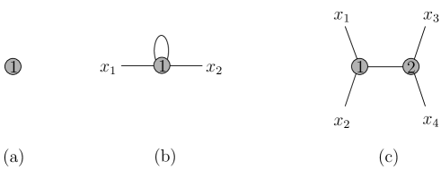
Figure 2: (a) An isolated vertex represented by $1\in\mathsf{S}(V)$; (b) A vertex with a self-loop and two external edges represented by $R_{1,1}\cdot(\phi(x_{1})\phi(x_{2}))\in\mathsf{S}(V)$; (c) A tree graph on two vertices and two external edges represented by $R_{1,2}\cdot(\phi(x_{1})\phi(x_{2})\otimes\phi(x_{3})\phi(x_{4}))\in\mathsf{S}(V)^{\otimes 2}$.

Figure 2 shows some examples of this correspondence.

Now, let us recall the definition of the componentwise product $\cdot:\mathsf{S}(V)^{\otimes v}\times\mathsf{S}(V)^{\otimes v}\to\mathsf{S}(V)^{\otimes v};(u_{1}\otimes\ldots\otimes u_{v},u^{\prime}_{1}\otimes\ldots\otimes u^{\prime}_{v})\mapsto u_{1}u^{\prime}_{1}\otimes\ldots\otimes u_{v}u^{\prime}_{v}$, where $u_{i},u^{\prime}_{j}$ denote monomials on the elementary field operators for all $1\leq i,j\leq v$. Clearly, combining several internal and external edges by multiplying their expressions in $\mathsf{S}(V)^{\otimes v}$ allows to build arbitrary graphs on $v$ vertices. Applying a given type of vertex functions $\nu^{\otimes v}$ to the resulting expression yields the value of the associated Feynman graph in the sense of Section II.1. Recall that the vertex functions carry a Feynman propagator for all assigned ends of edges (see equation (2)). Hence, the inverse Feynman propagator $G_{F}^{-1}$ in the definition of the elements $R_{i,j},R_{i,i}$ which represent internal edges, cancels one superfluous Feynman propagator.

For instance, let $\gamma$ denote an arbitrary graph on $v$ vertices and $e$ internal edges. For all $1\leq k\leq e$, let $R_{i_{k},j_{k}}$ represent an internal edge of $\gamma$ with $1\leq i_{k},j_{k}\leq v$. Also, for all $1\leq i\leq v$, let the vertex $i$ be assigned with the following $n_{i}\geq 0$ external edges $\phi(x_{1,i}),\ldots,\phi(x_{n_{i},i})$ with $\phi(x_{0,i}):=1$. In this context, we define the internal edge tensor associated with $\gamma$, $\mbox{int}_{1,\ldots,v}^{\gamma}\in\mathsf{S}(V)^{\otimes v}$, as follows:

$$\mbox{int}_{1,\ldots,v}^{\gamma}:=\prod_{k=1}^{e}R_{i_{k},j_{k}}\,.$$ (6)

Accordingly, we define the external edge tensor associated with $\gamma$, $\mbox{ext}_{1,\ldots,v}^{\gamma}\in\mathsf{S}(V)^{\otimes v}$, by inserting the external edges of the vertex $i$ in the $i$th tensor factor, for all $1\leq i\leq v$. That is,

$$\mbox{ext}_{1,\ldots,v}^{\gamma}:=\phi(x_{1,1})\ldots\phi(x_{n_{1},1})\otimes\ldots\otimes\phi(x_{1,v})\ldots\phi(x_{n_{v},v})\,,$$ (7)

where the operator labels are all distinct. Clearly, both $\mbox{int}_{1,\ldots,v}^{\gamma}$ and $\mbox{ext}_{1,\ldots,v}^{\gamma}$ are elements of $\mathsf{S}(V)^{\otimes v}$ which represent graphs themselves. In this context, the algebraic representation is so that the graph $\gamma$ is uniquely represented by a tensor $S^{\gamma}_{1,\ldots,v}\in\mathsf{S}(V)^{\otimes v}$ given by the (componentwise) product of $\mbox{int}_{1,\ldots,v}^{\gamma}$ by $\mbox{ext}_{1,\ldots,v}^{\gamma}$. That is,

$$S^{\gamma}_{1,\ldots,v}:=\mbox{int}_{1,\ldots,v}^{\gamma}\cdot\mbox{ext}_{1,\ldots,v}^{\gamma}\,.$$ (8)

For instance, Figure 3 shows a disconnected graph, while Figure 4 shows the associated internal and external edge tensors.

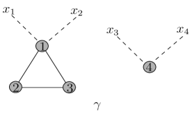
Figure 3: A disconnected graph represented by the tensor $S_{1,\ldots,4}^{\gamma}=\mbox{int}^{\gamma}_{1,\ldots,4}\cdot\mbox{ext}^{\gamma}_{1,\ldots,4}\in\mathsf{S}(V)^{\otimes 4}$.

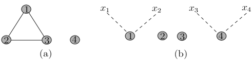
Figure 4: (a) The internal edge tensor associated with the graph $\gamma$: $\mbox{int}^{\gamma}_{1,\ldots,4}=R_{1,2}\cdot R_{1,3}\cdot R_{2,3}\in\mathsf{S}(V)^{\otimes 4}$; (b) The external edge tensor associated with the graph $\gamma$: $\mbox{ext}^{\gamma}_{1,\ldots,4}=\phi(x_{1})\phi(x_{2})\otimes 1\otimes 1\otimes\phi(x_{3})\phi(x_{4})\in\mathsf{S}(V)^{\otimes 4}$.

Moreover, the ordering of the tensor factors of $\mathsf{S}(V)^{\otimes v}$ determines the numbering of the vertices of a graph. Note, however, that when applying a given type of vertex functions $\nu^{\otimes v}$, all mutually isomorphic graphs contribute to the value of the same Feynman graph. In this context, let $\mathbb{C}\mathfrak{G}_{v}$ denote the $\mathbb{C}$-vector space on the set $\mathfrak{G}_{v}$ of all Feynman graphs (i.e., unnumbered graphs) on $v$ vertices. The subset of $\mathsf{S}(V)^{\otimes v}$ whose elements are so that the labels of the underlying elementary field operators are all distinct, may be clearly embedded in $\mathfrak{G}_{v}$ via the correspondence $\gamma\mapsto\bar{\gamma}$, where $\bar{\gamma}$ denotes the Feynman graph associated with $\gamma$. We will not point this out explicitly in the following.

Furthermore, let $v^{\prime}\geq v$ denote an integer. Let $X\subseteq\{1,\ldots,v^{\prime}\}$ be a set of cardinality $v$. Let $\sigma:\{1,\ldots,v\}\to X$ be a bijection. For all $v^{\prime}\geq v$, we define the following elements of $\mathsf{S}(V)^{\otimes v^{\prime}}$:

$$S_{\sigma(1),\ldots,\sigma(v)}^{\gamma}:=\mbox{int}^{\gamma}_{\sigma(1),\ldots,\sigma(v)}\cdot\mbox{ext}^{\gamma}_{\sigma(1),\ldots,\sigma(v)}\,,$$ (9)

where

$$\mbox{int}^{\gamma}_{\sigma(1),\ldots,\sigma(v)}:=\prod_{k=1}^{e}R_{\sigma(i_{k}),\sigma(j_{k})},$$ (10)

$$\mbox{ext}^{\gamma}_{\sigma(1),\ldots,\sigma(v)}:=\prod_{i=1}^{v^{\prime}}1^{\otimes\sigma(i)-1}\otimes\phi(x_{1,i})\ldots\phi(x_{n_{i},i})\otimes 1^{\otimes v-\sigma(i)}\,.$$ (11)

In terms of graphs, the tensor $S_{\sigma(1),\ldots,\sigma(v)}^{\gamma}$ represents a disconnected graph, say, $\gamma^{\prime}$, on $v^{\prime}$ vertices consisting of a graph isomorphic to $\gamma$ whose vertices take numbers from the set $X$ and $v^{\prime}-v$ isolated vertices taking numbers from the set $\{1,\ldots,v^{\prime}\}\backslash X$. Figure 5 shows an example. The interpretation of the tensors $\mbox{int}^{\gamma}_{\sigma(1),\ldots,\sigma(v)}$ and $\mbox{ext}^{\gamma}_{\sigma(1),\ldots,\sigma(v)}$ is analogous.

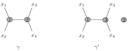
Figure 5: The graph $\gamma$ is represented by the tensor $S^{\gamma}_{1,2}\in\mathsf{S}(V)^{\otimes 2}$; The graph $\gamma^{\prime}$ is represented by the tensor $S^{\gamma}_{1,3}\in\mathsf{S}(V)^{\otimes 3}$ associated with $\gamma$ and the bijection $\sigma:\{1,2\}\to\{1,3\};1\mapsto 1,2\mapsto 3$.

III.2 Tensor algebra

We consider the tensor algebra $\mathsf{T}(\mathsf{S}(V))$ generated by the graded vector space $\mathsf{S}(V)$. We use the concatenation of tensors to define a non-associative product in $\mathsf{T}(\mathsf{S}(V))$. This may be interpreted in terms of graphs as the operation of gluing two graphs at a vertex.

Consider the tensor algebra on the graded vector space $\mathsf{S}(V)$: $\mathsf{T}(\mathsf{S}(V)):=\bigoplus_{k=1}^{\infty}\mathsf{S}(V)^{\otimes k}$. In $\mathsf{T}(\mathsf{S}(V))$ the multiplication $\bullet:\mathsf{T}(\mathsf{S}(V))\times\mathsf{T}(\mathsf{S}(V))\to\mathsf{T}(\mathsf{S}(V))$ is defined by concatenation of tensors (see Ref. k-theory, for instance):

$$(u_{1}\otimes\ldots\otimes u_{v})\bullet(u^{\prime}_{1}\otimes\ldots\otimes u^{\prime}_{v^{\prime}}):=u_{1}\otimes\ldots\otimes u_{v}\otimes u^{\prime}_{1}\otimes\ldots\otimes u^{\prime}_{v^{\prime}}\,,$$ (12)

where $u_{i}\,,u^{\prime}_{j}$ denote monomials on the elementary field operators for all $1\leq i\leq v$, $1\leq j\leq v^{\prime}$. We proceed to generalize the definition of the multiplication $\bullet$ to any two positions of the tensor factors. Let $\tau:\mathsf{S}(V)^{\otimes 2}\to\mathsf{S}(V)^{\otimes 2};u_{1}\otimes u_{2}\mapsto u_{2}\otimes u_{1}$. Moreover, define $\tau_{k}:=\operatorname{id}^{\otimes{k-1}}\otimes\tau\otimes\operatorname{id}^{\otimes{v-k-1}}:\mathsf{S}(V)^{\otimes v}\to\mathsf{S}(V)^{\otimes v}$ for all $1\leq k\leq v-1$ . In this context, for all $1\leq i\leq v$, $1\leq j\leq v^{\prime}$, define $\bullet_{i,j}:\mathsf{S}(V)^{\otimes v}\times\mathsf{S}(V)^{\otimes v^{\prime}}\to\mathsf{S}(V)^{\otimes v+v^{\prime}}$ by the following equation:

$$(u_{1}\otimes\ldots\otimes u_{v})\bullet_{i,j}(u^{\prime}_{1}\otimes\ldots\otimes u^{\prime}_{v^{\prime}}):=$$ (14)

$$(\tau_{v-1}\circ\ldots\circ\tau_{i})(u_{1}\otimes\ldots\otimes u_{v})\otimes(\tau_{1}\circ\ldots\circ\tau_{j-1})(u^{\prime}_{1}\otimes\ldots\otimes u^{\prime}_{v^{\prime}})$$

$$\quad=u_{1}\otimes\ldots\otimes\hat{u_{i}}\otimes\ldots\otimes u_{v}\otimes u_{i}\otimes u^{\prime}_{j}\otimes u^{\prime}_{1}\otimes\ldots\otimes\hat{u^{\prime}_{j}}\otimes\ldots\otimes u^{\prime}_{v^{\prime}}\,,$$

where $\hat{u_{i}}$ (resp. $\hat{u^{\prime}_{j}}$) means that $u_{i}$ (resp. $u^{\prime}_{j}$) is excluded from the sequence. In terms of the tensors $S^{\gamma}_{1,\ldots,v}\in\mathsf{S}(V)^{\otimes v}$ and $S^{\gamma^{\prime}}_{1,\ldots,v^{\prime}}\in\mathsf{S}(V)^{\otimes v^{\prime}}$ the equation above yields

$$S^{\gamma}_{1,\ldots,v}\bullet_{i,j}S^{\gamma^{\prime}}_{1,\ldots,v^{\prime}}:=S_{\sigma(1),\ldots,\sigma(v)}^{\gamma}\cdot S_{\sigma^{\prime}(1),\ldots,\sigma^{\prime}(v^{\prime})}^{\gamma^{\prime}}\,,$$ (15)

where $S_{\sigma(1),\ldots,\sigma(v)}^{\gamma},S_{\sigma^{\prime}(1),\ldots,\sigma^{\prime}(v^{\prime})}^{\gamma^{\prime}}\in\mathsf{S}(V)^{\otimes(v+v^{\prime})}$, $\sigma(k)=k$ if $1\leq k<i$, $\sigma(i)=v$, $\sigma(k)=k-1$ if $i<k\leq v$ and $\sigma^{\prime}(k)=k+v+1$ if $1\leq k<j$, $\sigma^{\prime}(j)=v+1$, $\sigma^{\prime}(k)=k+v$ if $j<k\leq v^{\prime}$. Clearly, $S_{1,\ldots,v}^{\gamma}\bullet_{i,j}S_{1,\ldots,v^{\prime}}^{\gamma^{\prime}}$ corresponds to a disconnected graph.

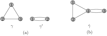
Figure 6: (a) The graphs represented by the tensors $S_{1,2,3}^{\gamma}\in\mathsf{S}(V)^{\otimes 3}$ and $S_{1,2}^{\gamma^{\prime}}\in\mathsf{S}(V)^{\otimes 2}$; (b) The graph represented by the tensor $S^{\hat{\gamma}}_{1,2,3,4}=S_{1,2,3}^{\gamma}\Diamond_{3,2}S_{1,2}^{\gamma^{\prime}}\in\mathsf{S}(V)^{\otimes 4}$.

Now, let $\cdot_{i}:=\operatorname{id}^{\otimes{i-1}}\otimes\cdot\otimes\operatorname{id}^{\otimes{v-i-1}}:\mathsf{S}(V)^{\otimes v}\to\mathsf{S}(V)^{\otimes(v-1)}$. In $\mathsf{T}(\mathsf{S}(V))$, for all $1\leq i\leq v$, $1\leq j\leq v^{\prime}$, define the following non-associative and non-commutative multiplication:

$$\Diamond_{i,j}:=\tau_{v+v^{\prime}-2}\circ\ldots\circ\tau_{v}\circ\cdot_{v}\circ\bullet_{i,j}:\mathsf{S}(V)^{\otimes v}\times\mathsf{S}(V)^{\otimes v^{\prime}}\to\mathsf{S}(V)^{\otimes(v+v^{\prime}-1)}\,.\\$$ (16)

The tensor $S^{\gamma}_{1,\ldots,v}\Diamond_{i,j}S^{\gamma^{\prime}}_{1,\ldots,v^{\prime}}$ represents the graph on $v+v^{\prime}-1$ vertices, say, $\hat{\gamma}$ obtained by gluing the vertex $i$ of $\gamma$ to the vertex $j$ of $\gamma^{\prime}$. Note that the subgraphs $\gamma$ and $\gamma^{\prime}$ of the graph $\hat{\gamma}$ share only the vertex $v+v^{\prime}-1$ (together with assigned external edges or self-loops) and no internal edges (distinct from self-loops). The vertex $v+v^{\prime}-1$ is clearly an articulation vertex of the graph $\hat{\gamma}$. Figure 6 shows an example.

IV A coalgebra structure on 1VI graphs

We give a coalgebra structure on 1VI Feynman graphs which is that of a cocommutative coassociative graded connected coalgebra. We generalize the coproduct to the algebraic representation. We emphasize that in the present section only graphs with no external edges nor self-loops are considered. Hence, in all that follows by graphs we mean graphs without external edges nor self-loops.

Let $\mathfrak{B}_{l,v}$ denote the set of all 1VI Feynman graphs on $l$ loops and $v$ vertices. Let $\mathbb{C}\mathfrak{B}_{l,v}$ denote the $\mathbb{C}$-vector space with the set $\mathfrak{B}_{l,v}$ as basis. Let $\mathbb{C}\mathfrak{B}:=\bigoplus_{v=1,l=0}^{\infty}\mathbb{C}\mathfrak{B}_{l,v}$. We define the following coalgebra structure on the graded vector space $\mathbb{C}\mathfrak{B}$:

• the coproduct $\vartriangle:\mathbb{C}\mathfrak{B}\to\mathbb{C}\mathfrak{B}\otimes\mathbb{C}\mathfrak{B}$ is defined as follows:

  $$\vartriangle(\bar{s}) := \bar{s}\otimes\bar{s}\,;$$ (17)

  $$\vartriangle(\bar{\gamma}) := \bar{s}\otimes\bar{\gamma}+\bar{\gamma}\otimes\bar{s}\quad\mbox{if}\quad\bar{\gamma}\neq\bar{s}\,,$$ (18)

  where $\bar{s}$ and $\bar{\gamma}$ denote a single vertex and an (unnumbered) 1VI graph on $v>1$ vertices, respectively. The coproduct $\vartriangle$ is clearly coassociative and cocommutative;

• the counit $\operatorname{\epsilon}:\mathbb{C}\mathfrak{B}\to\mathbb{C}$ is defined by

  $$\operatorname{\epsilon}(\bar{s}) := 1\,;$$ (19)

  $$\operatorname{\epsilon}(\bar{\gamma}) := 0\quad\mbox{if}\quad\bar{\gamma}\neq\bar{s}\,.$$ (20)

We grade the coalgebra $\mathbb{C}\mathfrak{B}$ as follows: if $\bar{\gamma}\in\mathfrak{B}_{l,v}$ then $\bar{\gamma}$ has degree $v-1$. $\mathbb{C}\mathfrak{B}$ is clearly connected for $\mathfrak{B}_{1,0}$ is a set with only one element, an isolated vertex.

We proceed to generalize the coproduct to the algebraic representation. Let $\mathscr{B}_{l,v}\subset\mathsf{S}(V)^{\otimes v}$ denote the vector space of all tensors representing 1VI graphs on $l$ loops and $v$ vertices. Let $\mathscr{B}:=\bigoplus_{v=1,l=0}^{\infty}\mathscr{B}_{l,v}\subset\mathsf{T}(\mathsf{S}(V))$. In $\mathscr{B}$ the analog of the coproduct $\vartriangle$ is the map $\bigtriangleup:\mathscr{B}\to\mathsf{T}(\mathsf{S}(V))$ defined by the following equations:

$$\bigtriangleup(1) := 1\otimes 1\,;$$ (21)

$$\bigtriangleup(B_{1,\ldots,v}^{\gamma}) := \frac{1}{v}\sum_{i=1}^{v}\bigtriangleup_{i}(B_{1,\ldots,v}^{\gamma})\quad\mbox{if}\quad v>1\,,$$ (22)

where $\gamma$ denotes a 1VI graph on $v$ vertices represented by $B_{1,\ldots,v}^{\gamma}\in\mathsf{S}(V)^{\otimes v}$. To define the maps $\bigtriangleup_{i}$ we introduce the following bijections:

• $\sigma_{i}:j\mapsto\left\{\begin{array}[]{ll}j&\mbox{if}\quad 1\leq j\leq i\\ j+1&\mbox{if}\quad i+1\leq j\leq v\\ \end{array}\right.$,

• $\nu_{i}:j\mapsto\left\{\begin{array}[]{ll}j&\mbox{if}\quad 1\leq j\leq i-1\\ j+1&\mbox{if}\quad i\leq j\leq v\\ \end{array}\right.\,.$

In this context, for all $1\leq i\leq v$ with $v>1$, the maps $\bigtriangleup_{i}:\mathsf{S}(V)^{\otimes v}\to\mathsf{S}(V)^{\otimes(v+1)}$ are defined by the following equation:

$$\bigtriangleup_{i}(B_{1,\ldots,v}^{\gamma}) := B_{\sigma_{i}(1),\ldots,\sigma_{i}(v)}^{\gamma}+B_{\nu_{i}(1),\ldots,\nu_{i}(v)}^{\gamma}$$ (23)

$$= B_{1,\ldots,\widehat{i+1},i+2,\ldots,v+1}^{\gamma}+B_{1,\ldots,\hat{i},i+1\ldots,v+1}^{\gamma}\,,$$ (24)

where $\hat{i}$ (resp. $\widehat{i+1}$) means that the index $i$ (resp. $i+1$) is excluded from the sequence. The tensor $B^{\gamma}_{1,\ldots,\hat{i},\ldots,v+1}$ (resp. $B_{1,\ldots,\widehat{i+1},i+2,\ldots,v+1}^{\gamma}$) is constructed from $B_{1,\ldots,v}^{\gamma}$ by transferring the monomial on the elementary field operators which occupies the $k$th tensor factor to the $(k+1)$th position for all $i\leq k\leq v$ (resp. $i+1\leq k\leq v$). Given a 1VI graph $\gamma$, one way to think about the map $\bigtriangleup_{i}$ is as the operation consisting of (a) splitting the vertex $i$ in two new vertices numbered $i$ and $i+1$; (b) transferring all the ends of edges assigned to the vertex $i$ to one of the two new vertices at a time.

Furthermore, given a bijection $\pi$ so that $i\notin\pi(\{1,\ldots,v\})\subset\{1,\ldots,v^{\prime}\}$, let $\bigtriangleup_{i}(B_{\pi(1),\ldots,\pi(v)}^{\gamma}):=B_{\nu_{i}(\pi(1)),\ldots,\nu_{i}(\pi(v))}^{\gamma}$. It is straightforward to verify that the maps $\bigtriangleup_{i}$ satisfy the following property:

$$\bigtriangleup_{i}\circ\bigtriangleup_{i}=\bigtriangleup_{i+1}\circ\bigtriangleup_{i}\,,$$ (25)

where we used the same notation for $\bigtriangleup_{i}:\mathsf{S}(V)^{\otimes v}\to\mathsf{S}(V)^{\otimes(v+1)}$ on the right of either side of the above equation and $\bigtriangleup_{i}:\mathsf{S}(V)^{\otimes(v+1)}\to\mathsf{S}(V)^{\otimes(v+2)}$ on the left of the lhs. Accordingly, $\bigtriangleup_{i+1}:\mathsf{S}(V)^{\otimes(v+1)}\to\mathsf{S}(V)^{\otimes(v+2)}$ on the rhs.

Now, for all $m>0$, define the $m$th iterate of $\bigtriangleup_{i}$, $\bigtriangleup_{i}^{m}:\mathsf{S}(V)^{\otimes v}\to\mathsf{S}(V)^{\otimes(v+m)}$, recursively as follows:

$$\bigtriangleup_{i}^{1} := \bigtriangleup_{i}\,;$$ (26)

$$\bigtriangleup_{i}^{m} := \bigtriangleup_{i}\circ\bigtriangleup_{i}^{m-1}\,,$$ (27)

where $\bigtriangleup_{i}:\mathsf{S}(V)^{\otimes(v+m-1)}\to\mathsf{S}(V)^{\otimes(v+m)}$ in formula (27). This can be written in $m$ different ways corresponding to the composition of $\bigtriangleup_{i}^{m-1}$ with each of the maps $\bigtriangleup_{j}:\mathsf{S}(V)^{\otimes(v+m-1)}\to\mathsf{S}(V)^{\otimes(v+m)}$ with $i\leq j\leq i+m-1$. These are all equivalent due to formula (25).

Extension to connected graphs

We now extend the maps $\bigtriangleup_{i}$ to the vector space of all tensors representing connected graphs on at least two vertices $\mathscr{B}^{*}:=\bigoplus_{k=1}^{\infty}\mathscr{B}^{\Diamond k}$. We proceed to define $\mathscr{B}^{\Diamond k}$.

First, given two sets $A_{v}\subset\mathsf{S}(V)^{\otimes v}$ and $B_{v^{\prime}}\subset\mathsf{S}(V)^{\otimes v^{\prime}}$, by $A_{v}\diamond_{i,j}B_{v^{\prime}}\subset\mathsf{S}(V)^{\otimes(v+v^{\prime}-1)}$; $i\in\{1,\ldots,v\},j\in\{1,\ldots,v^{\prime}\}$, denote the set of elements obtained by applying the map $\diamond_{i,j}$ to every ordered pair $(a\in A_{v},b\in B_{v^{\prime}})$.

For all $k\geq 1$, $l\geq 0$ and $v\geq k+1$, define ${\mathscr{B}^{*}}^{k}_{l,v}$ recursively as follows:

$${\mathscr{B}^{*}}^{1}_{l,v}=\biggl{\{}\mathscr{B}_{l,v}\biggr{\}}\,;$$

$${\mathscr{B}^{*}}^{2}_{l,v} = \biggl{\{}\mathscr{B}_{l-l^{\prime},v-v^{\prime}}\diamond_{i,j}{\mathscr{B}^{*}}^{1}_{l^{\prime},v^{\prime}+1}\quad\mbox{for all}\quad l^{\prime}=0,\ldots,l,v^{\prime}=1,\ldots,v-2,i=1,\ldots,v-v^{\prime},j=1,\ldots,v^{\prime}+1\biggr{\}}\,;$$

$${\mathscr{B}^{*}}^{k}_{l,v} = \biggl{\{}\mathscr{B}_{l-l^{\prime},v-v^{\prime}}\diamond_{i,j}{\mathscr{B}^{*}}^{k-1}_{l^{\prime},v^{\prime}+1}\quad\mbox{for all}\quad l^{\prime}=0,\ldots,l,v^{\prime}=k-1,\ldots,v-2,i=1,\ldots,v-v^{\prime},j=1,\ldots,v^{\prime}+1\biggr{\}}\,.$$

Let

$${{\mathscr{B}^{\prime}}^{*}}^{k}_{l,v}=\bigcup_{\pi\in S_{v}}\biggl{\{}S^{\gamma}_{\pi(1),\ldots,\pi(v)}|S^{\gamma}_{1,\ldots,v}\in{\mathscr{B}^{*}}^{k}_{l,v}\biggr{\}}\,,$$

where $S_{v}$ denotes the symmetric group on the set $\{1,\ldots,v\}$ and $S^{\gamma}_{\pi(1),\ldots,\pi(v)}$ is given by formula (9). Finally, for all $k\geq 1$, define

$$\mathscr{B}^{\diamond k}:=\bigoplus_{l=0,v=k+1}^{\infty}{{\mathscr{B}^{\prime}}^{*}}^{k}_{l,v}\,.$$

The elements of $\mathscr{B}^{\diamond k}$ are clearly tensors representing connected graphs on $k$ 1VI components (i.e., maximal 1VI subgraphs handbook ). By equations (16) and (9), these may be seen as monomials on tensors representing 1VI graphs, say, $B_{\sigma(1),\ldots,\sigma(v)}^{\gamma}$, with the componentwise product $\cdot:\mathsf{S}(V)^{\otimes v}\times\mathsf{S}(V)^{\otimes v}\to\mathsf{S}(V)^{\otimes v}$ so that repeated indices correspond to articulation vertices of the associated graphs. In this context, an arbitrary connected graph, say, $\gamma$, on $v\geq 2$ vertices and $k\geq 1$ 1VI components yields

$$\prod_{a=1}^{k}B_{\sigma_{a}(1),\ldots,\sigma_{a}(v_{a})}^{\gamma_{a}}\,,$$

where for all $1\leq a\leq k$, $B_{\sigma_{a}(1),\ldots,\sigma_{a}(v_{a})}^{\gamma_{a}}\in\mathsf{S}(V)^{\otimes v}$, $\gamma_{a}$ is a 1VI graph on $2\leq v_{a}\leq v$ vertices represented by $B_{1,\ldots,v_{a}}^{\gamma_{a}}\in\mathsf{S}(V)^{\otimes v_{a}}$ and $\sigma_{a}:\{1,\ldots,v_{a}\}\to X_{a}\subset\{1,\ldots,v\}$ is a bijection.

We now extend the map $\bigtriangleup:=\frac{1}{v}\sum_{i=1}^{v}\bigtriangleup_{i}$ to $\mathscr{B}^{*}$ by requiring the maps $\bigtriangleup_{i}$ to satisfy the following condition:

$$\bigtriangleup_{i}(\prod_{a=1}^{k}B_{\sigma_{a}(1),\ldots,\sigma_{a}(v_{a})}^{\gamma_{a}}):=\prod_{a=1}^{k}\bigtriangleup_{i}(B_{\sigma_{a}(1),\ldots,\sigma_{a}(v_{a})}^{\gamma_{a}})\,.$$ (28)

Given a connected graph $\gamma^{\prime}$, the map $\bigtriangleup_{i}$ may be thought of as a way of (a) splitting the vertex $i$ in two new vertices numbered $i$ and $i+1$; (b) distributing the 1VI components sharing the vertex $i$ between the two new ones in all possible ways. Analogously, the action of the maps $\bigtriangleup_{i}^{m}$ consists of (a) splitting the vertex $i$ in $m+1$ new vertices numbered $i,i+1,\ldots,i+m$; (b) distributing the 1VI components sharing the vertex $i$ between the $m+1$ new ones in all possible ways.

V Linear maps

We give the linear maps to be used in the following to generate 1VI and 1PI graphs.

We begin by recalling the definition of the truncated coproduct given in Section VI C of Ref. MeOe:npoint, . The coproduct restricted to the subspace $\mathsf{S}^{n}(V)\subset\mathsf{S}(V)$ is a map $\mathsf{S}^{n}(V)\to\bigoplus_{i=0}^{n}\mathsf{S}^{i}(V)\otimes\mathsf{S}^{n-i}(V)$. Removing those components of the direct sum where at least one of the target tensor factors is $\mathsf{S}^{0}(V)$ yields the following map, called truncated coproduct:

$${\Delta}_{\geq 1}:\mathsf{S}^{n}(V)\to\bigoplus_{i=1}^{n-1}\mathsf{S}^{i}(V)\otimes\mathsf{S}^{n-i}(V)\,.$$

For instance,

$$\operatorname{\Delta}_{\geq 1}(1)=0,\qquad\operatorname{\Delta}_{\geq 1}(\phi(x))=0,$$

$$\operatorname{\Delta}_{\geq 1}(\phi(x)\phi(y))=\phi(x)\otimes\phi(y)+\phi(y)\otimes\phi(x)\,.$$

Furthermore, we define the maps ${Q_{i}}^{(\rho)}_{\geq 1}$ in analogy with the maps $Q_{i}$ given in Section IV of Ref. MeOe:npoint, . To this end, we combine the elements $R_{i,i+1}^{\rho}$ (viewed as operators on $\mathsf{S}(V)^{\otimes v}$ by multiplication) with the truncated coproduct applied to the $i$th tensor factor of $\mathsf{S}(V)^{\otimes v}$, i.e., ${\Delta_{i}}_{\geq 1}:=\operatorname{id}^{\otimes{i-1}}\otimes{\Delta}_{\geq 1}\otimes\operatorname{id}^{\otimes{v-i}}$. That is, for all $1\leq i\leq v$, define

$${Q_{i}}^{(\rho)}_{\geq 1}:=\frac{1}{2(\rho-1)!}R_{i,i+1}^{\rho}\circ{\Delta_{i}}_{\geq 1}:\mathsf{S}(V)^{\otimes v}\to\mathsf{S}(V)^{\otimes{v+1}}\,.$$

In terms of graphs, the maps ${Q_{i}}^{(\rho)}_{\geq 1}$ are the algebraic equivalent of the maps ${q_{i}}^{(\rho)}_{\geq 1}$ given in Ref. Me:biconn, . We refer the reader to that paper for the precise definition. In plain English, the maps ${Q_{i}}^{(\rho)}_{\geq 1}$ produce a graph with $v+1$ vertices from one with $v$ vertices in the following way:

1. split the vertex $i$ into two new vertices numbered $i$ and $i+1$;

2. distribute the ends of edges ending on the split vertex between the two new ones in all possible ways so that each vertex is assigned with at least one end of edges;

3. connect the two new vertices with $\rho$ internal edges.

For $\rho=1$, on the algebraic level, the definition of the maps ${Q_{i}}^{(1)}_{\geq 1}$ (or $Q_{i}$ of Ref. MeOe:npoint, ) generalizes the application $L=(\phi\otimes\phi)\cdot\Delta$ given in Section 3 of Ref. Liv:rigidity, . On the level of graphs, this definition generalizes the fundamental operation given in Ref. 103, to all partitions of the set of ends of edges assigned to the vertex $i$.

Figure 7: The linear combination of graphs obtained by applying $\sum_{i=1}^{2}{Q_{i}}^{(1)}_{\geq 1}$ to a cycle on two vertices.

For instance, to illustrate the action of the maps ${Q_{i}}^{(1)}_{\geq 1}$, let $\gamma$ be a cycle on two vertices represented by $B^{C_{2}}_{1,2}=R_{1,2}^{2}\in\mathsf{S}(V)^{\otimes 2}$. Applying $\sum_{i=1}^{2}{Q_{i}}^{(1)}_{\geq 1}$ to $\gamma$ yields:

$$\sum_{i=1}^{2}{Q_{i}}^{(1)}_{\geq 1}(B^{C_{2}}_{1,2}) = \frac{1}{2}(R_{1,2}\circ{\operatorname{\Delta}_{1}}_{\geq 1}+R_{2,3}\circ{\operatorname{\Delta}_{2}}_{\geq 1})(R_{1,2}^{2})$$ (29)

$$= 2R_{1,2}\cdot R_{2,3}\cdot R_{1,3}\,.$$

Figure 7 shows the linear combination of graphs given by equation (29).

Furthermore, on $\mathscr{B}^{*}$ we define the maps ${\hat{Q_{i}}}^{(\rho)}_{\geq 1}$ as follows:

$${\hat{Q_{i}}}^{(\rho)}_{\geq 1}(\prod_{a=1}^{k}B_{\sigma_{a}(1),\ldots,\sigma_{a}(v_{a})}^{\gamma_{a}}):=\frac{1}{2(\rho-1)!}R_{i,i+1}^{\rho}\prod_{a=1}^{k}{\Delta_{i}}_{\geq 1}(B_{\sigma_{a}(1),\ldots,\sigma_{a}(v_{a})}^{\gamma_{a}})\,.$$ (30)

We now combine the maps $\bigtriangleup_{i}^{m}$ with tensors representing 1VI graphs in order to produce connected graphs.

Fix integers $v,v^{\prime}\geq 1$ and $1\leq i\leq v^{\prime}$. Let $\pi_{i}:\{1,\ldots,v\}\to\{i,i+1,\ldots,i+v-1\}$ be any bijection. Let $\gamma\in\mathfrak{B}$ be a 1VI graph on $v$ vertices represented by the tensor $B_{1,\ldots,v}^{\gamma}\in\mathsf{S}(V)^{\otimes v}$. The tensors $B_{\pi_{i}(1),\ldots,\pi_{i}(v)}^{\gamma}\in\mathsf{S}(V)^{v+v^{\prime}-1}$ (given by formula (9)) may be viewed as operators acting on $\mathsf{S}(V)^{v+v^{\prime}-1}$ by multiplication. In this context, consider the following maps given by the composition of $B_{\pi_{i}(1),\ldots,\pi_{i}(v)}^{\gamma}$ with $\bigtriangleup_{i}^{v-1}$:

$$B_{\pi_{i}(1),\ldots,\pi_{i}(v)}^{\gamma}\circ\bigtriangleup_{i}^{v-1}:\mathsf{S}(V)^{\otimes v^{\prime}}\to\mathsf{S}(V)^{\otimes{v+v^{\prime}-1}}\,.$$

In terms of graphs, the maps $B_{\pi_{i}(1),\ldots,\pi_{i}(v)}^{\gamma}\circ\bigtriangleup_{i}^{v-1}$ are the algebraic equivalent of the maps $r_{i}^{G}$ given in Ref. Me:biconn, . We refer the reader to that paper for the precise definition. In plain English, the maps $B_{\pi_{i}(1),\ldots,\pi_{i}(v)}^{\gamma}\circ\bigtriangleup_{i}^{v-1}$ produce a connected graph with $v+v^{\prime}-1$ vertices from one with $v^{\prime}$ vertices in the following way:

1. split the vertex $i$ into $v$ new vertices numbered $i$, $i+1$,$\ldots$, $i+v-1$;

2. distribute the 1VI components sharing the split vertex between the $v$ new ones in all possible ways;

3. merge the $v$ new vertices into the graph $\gamma$.

Figure 8: The linear combination of graphs obtained by applying the map $R_{3,4}\circ\bigtriangleup_{3}$ to the articulation vertex of a graph consisting of two triangles sharing a vertex.

To illustrate the action of the maps $B_{\pi_{i}(1),\ldots,\pi_{i}(v)}^{\gamma}\circ\bigtriangleup_{i}$, let $\gamma$ be a graph consisting of two triangles sharing a vertex. Let this be represented by $B^{C_{3}}_{1,2,3}\cdot B^{C_{3}}_{3,4,5}\in\mathsf{S}(V)^{\otimes 5}$, where $C_{3}$ denotes a triangle represented by $B^{C_{3}}_{1,2,3}=R_{1,2}\cdot R_{2,3}\cdot R_{1,3}\in\mathsf{S}(V)^{\otimes 3}$. Let $T_{2}$ denote a $2$-vertex tree represented by $B^{T_{2}}_{1,2}=R_{1,2}\in\mathsf{S}(V)^{\otimes 2}$. Applying the map $R_{3,4}\circ\bigtriangleup_{3}$ to $\gamma$ yields:

$$R_{3,4}\circ\bigtriangleup_{3}(B^{C_{3}}_{1,2,3}\cdot B^{C_{3}}_{3,4,5})=R_{3,4}\cdot\bigtriangleup_{3}(B^{C_{3}}_{1,2,3})\cdot\bigtriangleup_{3}(B^{C_{3}}_{3,4,5})$$ (31)

$$= R_{3,4}\cdot(B^{C_{3}}_{1,2,3}+B^{C_{3}}_{1,2,4})\cdot(B^{C_{3}}_{3,5,6}+B^{C_{3}}_{4,5,6})$$

$$= R_{3,4}\cdot B^{C_{3}}_{1,2,3}\cdot B^{C_{3}}_{3,5,6}+R_{3,4}\cdot B^{C_{3}}_{1,2,3}\cdot B^{C_{3}}_{4,5,6}+R_{3,4}\cdot B^{C_{3}}_{1,2,4}\cdot B^{C_{3}}_{3,5,6}+R_{3,4}\cdot B^{C_{3}}_{1,2,4}\cdot B^{C_{3}}_{4,5,6}\,.$$

Figure 8 shows the linear combination of graphs given by equation (31) after noticing that the first and fourth terms as well as the second and third correspond to isomorphic graphs.

VI Generating 1VI and 1PI graphs

We give recursion formulas to generate all 1VI and all 1PI graphs (with non-vanishing loop number) directly in the algebraic representation given in Ref. MeOe:npoint, .

VI.1 1-vertex irreducible graphs

We express Theorem 4 of Ref. Me:biconn, in a completely algebraic language.

Theorem 1.

For all integers $l\geq 0$ and $v>1$, define $\mathfrak{V}_{1,\ldots,v}^{l,v}\in\mathsf{S}(V)^{\otimes v}$ by the following recursion relation:

$$\mathfrak{V}^{l,2}_{1,2} := \frac{1}{2(l+1)!}R_{1,2}^{l+1}\,;$$ (32)

$$\mathfrak{V}^{0,v}_{1,\ldots,v} := 0\,,\quad v>2\,;$$ (33)

$$\mathfrak{V}^{l,v}_{1,\ldots,v} := \frac{1}{l+v-1}\biggl{(}\sum_{\rho=1}^{l}\sum_{i=1}^{v-1}{Q_{i}}^{(\rho)}_{\geq 1}(\mathfrak{V}^{l+1-\rho,v-1}_{1,\ldots,v-1})+\sum_{k=2}^{v-2}\sum_{\rho=1}^{l-k+1}\hat{Q}^{(\rho)}_{{v-1}_{\geq 1}}(\mathfrak{B}^{l+1-\rho,v-1,k}_{1,\ldots,v-1})\biggr{)}\,,\quad v>2\,,$$ (34)

where for all integers $k>1$, $v\geq k+1$ and $l\geq k$, $\mathfrak{B}^{l,v,k}_{1,\ldots,v}$ is given by the following recursion relation:

$$\mathfrak{B}^{l,v,2}_{1,\ldots,v}:=\frac{1}{l+v-1}\sum_{l^{\prime}=1}^{l-1}\sum_{v^{\prime}=2}^{v-1}\sum_{i=1}^{v^{\prime}}\sum_{j=1}^{v-v^{\prime}+1}\biggl{(}(l^{\prime}+v^{\prime}-1)\mathfrak{V}^{l^{\prime},v^{\prime}}_{1,\ldots,v^{\prime}}\Diamond_{i,j}\mathfrak{V}^{l-l^{\prime},v-v^{\prime}+1}_{1,\ldots,v-v^{\prime}+1}\biggr{)}\,;$$ (35)

$$\mathfrak{B}^{l,v,k}_{1,\ldots,v}:=\frac{1}{l+v-1}\sum_{l^{\prime}=1}^{l-1}\sum_{v^{\prime}=2}^{v-1}\sum_{i=1}^{v^{\prime}}\biggl{(}(l^{\prime}+v^{\prime}-1)\mathfrak{V}^{l^{\prime},v^{\prime}}_{1,\ldots,v^{\prime}}\Diamond_{i,v-v^{\prime}+1}\mathfrak{B}^{l-l^{\prime},v-v^{\prime}+1,k-1}_{1,\ldots,v-v^{\prime}+1}\biggr{)}\,.$$ (36)

Then, for fixed values of $v$ and $l$, $\mathfrak{V}^{l,v}_{1,\ldots,v}$ is the weighted sum over all 1VI Feynman graphs with $l$ loops, $v$ vertices and no external edges nor self-loops, each with weight given by the inverse of its symmetry factor.

In formula (34), the $\hat{Q}^{(\rho)}_{{v-1}_{\geq 1}}$ summand does not appear when $v<4$ or $l<2$.

Proof.

The result follows from Theorem 4 of Ref. Me:biconn, . This is due to the correspondence between graphs and elements of $\mathsf{S}(V)^{\otimes v}$ and the fact that the definitions of the maps ${Q_{i}}^{(\rho)}_{\geq 1}$ and ${\hat{Q_{i}}}^{(\rho)}_{\geq 1}$ mirror those of the maps ${q_{i}}^{(\rho)}_{\geq 1}$ and ${\hat{q_{i}}}^{(\rho)}_{\geq 1}$, respectively, given in that paper. ∎

VI.2 1-particle irreducible graphs

We use Theorem 1 and the maps $B_{\pi_{i}(1),\ldots,\pi_{i}(v)}^{\gamma}\circ\bigtriangleup_{i}^{v-1}$ given in Section V to generate all 1PI graphs following Ref. Me:biconn, .

Theorem 2.

For all integers $l>0$ and $v>1$, define $\mathfrak{I}^{v,l,}_{1,\ldots,v}\in\mathsf{S}(V)^{\otimes v}$ by the following recursion relation:

$$\mathfrak{I}^{l,2}_{1,2} := \mathfrak{V}^{l,2}_{1,2}\,;$$ (37)

$$\mathfrak{I}^{l,v}_{1,\ldots,v} := \mathfrak{V}^{l,v}_{1,\ldots,v}+\frac{1}{l+v-1}\cdot\sum_{l^{\prime}=1}^{l-1}\sum_{v^{\prime}=2}^{v-1}\sum_{i=1}^{v-v^{\prime}+1}\biggl{(}(l^{\prime}+v^{\prime}-1)\mathfrak{V}^{l^{\prime},v^{\prime}}_{\pi_{i}(1),\ldots,\pi_{i}(v^{\prime})}\circ\bigtriangleup_{i}^{v^{\prime}-1}(\mathfrak{I}^{l-l^{\prime},v-v^{\prime}+1}_{1,\ldots,v-v^{\prime}+1})\biggr{)},v>2\,.$$ (38)

Then, for fixed values of $v$ and $l$, $\mathfrak{I}^{l,v}_{1,\ldots,v}$ is the weighted sum over all 1PI Feynman graphs with $l$ loops, $v$ vertices and no external edges nor self-loops, each with weight given by the inverse of its symmetry factor.

Proof.

The result follows from Theorem 10 of Ref. Me:biconn, . This is due to the correspondence between graphs and elements of $\mathsf{S}(V)^{\otimes v}$ and the fact that the definition of the maps $B_{\pi_{i}(1),\ldots,\pi_{i}(v)}^{\gamma}\circ\bigtriangleup_{i}^{v-1}$ mirrors that of the maps $r_{i}^{G}$ of that paper. ∎

We now consider 1PI graphs with self-loops and external edges allowed. Recall the elements $T_{i}:=\frac{1}{2}R_{i,i}\in\mathsf{S}(V)^{\otimes v}$ with $1\leq i\leq v$, given in Ref. MeOe:loop, . Moreover, let $\mathsf{R}^{k}(V)$ denote the vector space generated by $T_{1}^{k}$, with $T_{1}^{0}=1$. Let $\mathsf{R}(V)=\bigoplus_{k=0}^{\infty}\mathsf{R}^{k}(V)\subset\mathsf{S}(V)$, where $\mathsf{R}^{0}(V):=\mathbb{C}1$. Now, define $\delta:\mathsf{R}(V)\to\mathsf{R}(V)\otimes\mathsf{R}(V);1\mapsto 1\otimes 1;T_{1}^{k}\mapsto(T_{1}+T_{2})^{k}$. The map $\delta$ is clearly coassociative: $(\delta\otimes\operatorname{id})\circ\delta=(\operatorname{id}\otimes\delta)\circ\delta$. Moreover, for all $m\geq 0$, define $\delta^{m}:\mathsf{R}(V)\to\mathsf{R}(V)^{\otimes(m+1)}$ as follows: $\delta^{0}:=\operatorname{id}$ and $\delta^{m}:=(\delta\otimes\operatorname{id}^{\otimes(m-1)})\circ\delta^{m-1}$. The proposition is now established.

Proposition 3.

Fix an integer $n\geq 0$ as well as operator labels $x_{1},\ldots,x_{n}$. For all integers $l\geq 1$, $l^{\prime}\geq 0$ and $v\geq 1$, define $\Gamma^{l+l^{\prime},v}:\mathsf{S}(V)\to\mathsf{S}(V)^{\otimes v}$ as follows:

$$\Gamma^{l^{\prime},1} := \frac{1}{l^{\prime}!}T_{1}^{l^{\prime}}\circ\operatorname{id}\,;$$ (39)

$$\Gamma^{l+l^{\prime},v} := \frac{1}{l^{\prime}!}(\mathfrak{I}^{l,v}_{1,\ldots,v}\cdot\delta^{v-1}(T_{1}^{l^{\prime}}))\circ\operatorname{\Delta}^{v-1}\,,v\geq 2\,.$$ (40)

Then, $\Gamma^{l+l^{\prime},v}(\phi(x_{1})\cdots\phi(x_{n}))$ is the weighted sum over all 1PI Feynman graphs with $l$ loops (excluding self-loops), $l^{\prime}$ self-loops, $v$ vertices and $n$ external edges whose end points are labeled $x_{1},\dots,x_{n}$, each with weight given by the inverse of its symmetry factor.

Proof.

Clearly, $\delta^{v-1}(T_{1}^{l^{\prime}})=\sum_{{l^{\prime}}_{1},\ldots,{l^{\prime}}_{v}}\binom{l^{\prime}}{{l^{\prime}}_{1},\ldots,{l^{\prime}}_{v}}T_{1}^{{l^{\prime}}_{1}}\cdot\ldots\cdot T_{v}^{{l^{\prime}}_{v}}$, where the sum runs over all partitions of ${l^{\prime}}$ into $v$ non-negative integers. That is, for all $i=1,\ldots,v$, $l^{\prime}_{i}\geq 0$ with $\sum_{i}^{v}{l^{\prime}}_{i}=l^{\prime}$. Therefore, the result follows straightforwardly from the symmetry property of the multinomial coefficients: $\binom{l^{\prime}}{{l^{\prime}}_{1},\ldots,{l^{\prime}}_{v}}=\binom{l^{\prime}}{{l^{\prime}}_{\sigma(1)},\ldots,{l^{\prime}}_{\sigma(v)}}$, where $\sigma$ denotes any permutation of $\{1,\ldots,v\}$. ∎

VI.3 1PI $n$-point functions

We turn to the interpretation of $\Gamma^{l+l^{\prime},v}$ given by equation (40) in terms of Feynman graphs and $n$-point functions. We emphasize that the discussion here applies only to bare $n$-point functions for renormalization is outside the scope of the present work. Moreover, the results are valid for any quantum field theory.

In all that follows, let $l$ and $l^{\prime}$ denote the loop number (excluding self-loops) and the number of self-loops, respectively, of any Feynman graph. Now, by $\nu_{{\tiny\mbox{1PI}}}$, denote the 1PI vertex functions, i.e., the interaction vertices of each of the terms in the perturbative expansion of the 1PI $n$-point functions. By $\tau^{l+l^{\prime},v}$, denote the $l+l^{\prime}$-loop and $v$-vertex contribution to the ensemble $\tau$ of 1PI $n$-point functions. The $l+l^{\prime}$-loop order contribution $\tau^{l+l^{\prime}}$ to $\tau$ and $\tau$ itself, are given by

$$\tau^{l+l^{\prime}}=\sum_{v=1}^{\infty}\tau^{l+l^{\prime},v},\qquad\tau=\sum_{l+l^{\prime}=0}^{\infty}\tau^{l+l^{\prime}}.$$

All vertex order contributions are captured by the following corollary.

Corollary 4.

For $v\geq 1$:

$$\tau^{l+l^{\prime},v}=\nu_{{\tiny\mbox{1PI}}}^{\otimes v}\circ\Gamma^{l+l^{\prime},v}.$$

- (1) M. J. Atallah and S. Fox, editors. Algorithms and Theory of Computation Handbook. CRC Press, Inc., Boca Raton, FL, USA, 1998. Produced by S. Lassandro.
- (2) C. Brouder. Quantum field theory meets Hopf algebra. Math. Nachr. 282, No. 12:1664–1690, 2009.
- (3) C. Brouder, A. Frabetti, B. Fauser, and R. Oeckl. Quantum field theory and Hopf algebra cohomology. J. Phys., A 37:5895–5927, 2004.
- (4) C. Brouder and R. Oeckl. Quantum groups and quantum field theory: the free scalar field. Mathematical physics research on the leading edge, 63–90, Nova Sci. Publ., Hauppauge, NY, 2004.
- (5) J. Cuntz, R. Meyer, and J. M. Rosenberg. Topologival and bivariant K-theory. Oberwolfach Seminars Volume 36, Birkhäuser, Berlin, 2007.
- (6) D. Eisenbud. Commutative Algebra with a view toward Algebraic Geometry. Springer, Berlin, 1995.
- (7) H. Glover, J. Huneke, and C. Wang. 103 graphs that are irreducible for the projective plane. J. Combin. Theory Ser. B, 27:332–370, 1979.
- (8) C. Itzykson and J.-B. Zuber. Quantum Field Theory. McGraw-Hill, New York, 1980.
- (9) C. Kassel. Quantum Groups. Springer-Verlag, New York, Inc, 1995.
- (10) H. Kleinert and V. Schulte-Frohlinde. Critical properties of theories. World Scientific Publishing Company; 1st edition, 2001.
- (11) M. Livernet. A rigidity theorem for prelie algebras. Journal of Pure and Applied Algebra 207, 207:1–18, 2006.
- (12) J.-L. Loday. Cyclic Homology. Springer, Berlin, 1998.
- (13) Â. Mestre. On the decomposition of connected graphs into their biconnected components. arXiv:1001.3163v2 [math.CO], 2010.
- (14) Â. Mestre and R. Oeckl. Combinatorics of -point functions via Hopf algebra in quantum field theory. J. Math. Phys., 47:052301, 2006.
- (15) Â. Mestre and R. Oeckl. Generating loop graphs via Hopf algebra in quantum field theory. J. Math. Phys., 47:122302, 2006.