Ultrafast X-ray pulse measurement method

Abstract

In this paper we describe a measurement technique capable of resolving femtosecond X-ray pulses from XFEL facilities. Since these ultrashort pulses are themselves the shortest event available, our measurement strategy is to let the X-ray pulse sample itself. Our method relies on the application of a ”fresh” bunch technique, which allows for the production of a seeded X-ray pulse with a variable delay between seed and electron bunch. The shot-to-shot averaged energy per pulse is recorded. It turns out that one actually measures the autocorrelation function of the X-ray pulse, which is related in a simple way to the actual pulse width. For implementation of the proposed technique, it is sufficient to substitute a single undulator segment with a short magnetic chicane. The focusing system of the undulator remains untouched, and the installation does not perturb the baseline mode of operation. We present a feasibility study and we make exemplifications with typical parameters of an X-ray FEL.

DEUTSCHES ELEKTRONEN-SYNCHROTRON

Ein Forschungszentrum der Helmholtz-Gemeinschaft

DESY 10-008

January 2010

Ultrafast X-ray pulse measurement method

Gianluca Geloni,

European XFEL GmbH, Hamburg

Vitali Kocharyan and Evgeni Saldin

Deutsches Elektronen-Synchrotron DESY, Hamburg ISSN 0418-9833 NOTKESTRASSE 85 - 22607 HAMBURG

1 Introduction and method

Figure 1: Experimental layout for ultra-short X-ray pulse-measurement using ”fresh” bunch technique. Pulse and electron bunch are separated at the exit of first part of undulator, one is variably delayed with respect to the other. Modulation of the electron bunch is washed out. X-ray pulse and ”fresh” electron bunch are overlapped in the second part of undulator. The averaged X-ray pulse energy at the exit of setup is measured versus delay, yielding the autocorrelation trace.

The measurement of X-ray pulses on the femtosecond time scale constitutes an unresolved problem. It is possible to create sub-ten femtosecond X-ray pulses from XFELs, but not to measure them. In fact, conventional photodetectors and streak-camera detectors do not have a fast enough response time to characterize ultrashort radiation pulses. For example, the rise time of the best streak-cameras approaches $100$ fs, far too slow to resolve femtosecond pulses. Special measurement techniques are needed. In this paper we propose a new method for the measurement of the duration of femtosecond X-ray pulses from XFELs. The method is based on the measurement of the autocorrelation function of the X-ray pulses. The setup in Fig. 1, similar to that described in OUR01 , may be used to this purpose. The electron bunch enters the first part of the baseline undulator and produces SASE radiation with ten MW-level power. After the first part of the undulator, the electron bunch is guided through a short magnetic chicane whose function is both, to wash out the electron bunch modulation, and to create the necessary offset to install an X-ray optical delay line. The chicane is short enough to be installed in the space of a single XFEL segment, as shown in Fig. 2, and does not perturb the focusing structure of the machine. The optical delay line is sketched in Fig. 3, and has already been discussed in OUR02 .

Figure 2: Installation of a magnetic delay in the baseline XFEL undulator.

Figure 3: X-ray optical system for delaying the SASE pulse with respect to the electron bunch. The X-ray optical system can be installed within the magnetic chicane between first and second part of the undulator.

Figure 4: Sketch of X-ray intensity autocorrelation measurement using tunable X-ray optical delay line within magnetic chicane. This autocorrelator produces complete autocorrelation trace.

After the chicane, the electron beam and the X-ray radiation pulse produced in the first part of the undulator enter the second part of undulator, which is resonant at the same wavelength. In the second part of the undulator the first X-ray pulse acts as a seed and overlaps to the lasing part of electron bunch. Therefore, the output power rapidly grows up to the GW-level. First and second undulator parts are identical and operate in the linear FEL amplification regime. The relative delay between electron bunch and seed X-ray pulse can be varied by the X-ray optical delay line installed within the magnetic chicane, as illustrated in Fig. 4. Within the 1D FEL theory, which is not too far from reality for the SASE X-ray case with a large diffraction parameter, one can write the shot-to-shot averaged power in the pulse from the first part of the undulator as

$$\left<P(t)\right>=P_{0}\exp\left[2L_{w}\mathrm{Re}(\Lambda(t))\right]$$ (3)

where $P_{0}$ is the equivalent shot-nose power, $L_{w}=36$ m (6 cells) is the length of the two identical undulator parts and $\mathrm{Re}(\Lambda(t))$ is the time-dependent field growth-rate. Similarly, the shot-to-shot averaged power in the pulse from the second part of the undulator, which is seeded with $\left<P(t-\tau)\right>$, $\tau$ being the variable delay, can be written as

$$\left<P_{2}(t,\tau)\right>=\left<P(t-\tau)\right>\exp\left[2L_{w}\mathrm{Re}(\Lambda(t))\right]=\frac{1}{P_{0}}\left<P(t-\tau)\right>\left<P(t)\right>~{}.$$ (4)

The subsequent measurement procedure consists in recording the shot-to-shot averaged energy per pulse at the exit of the second part of the undulator as a function of the relative delay between electron bunch and seed X-ray pulse, with the help of an integrating photodetector. This yields the autocorrelation function

$$A(\tau)=\int_{-\infty}^{\infty}dt\left<P(t-\tau)\right>\left<P(t)\right>~{}.$$ (5)

Autocorrelation measurements are well known methods in laser physics. Early on, it was realized that the only event fast enough to measure an ultrashort pulse is the pulse itself. A number of schemes have been developed over the past decades to better measure ultrashort laser pulses. Most of them have been experimental implementations and variations of autocorrelators, i.e. devices capable of measuring the autocorrelation function of a given pulse, Eq. (5). Our scheme actually provides a device capable of performing an intensity autocorrelation measurement.

Figure 5: Experimental layout for measuring the optical pulse intensity versus time. At optical frequencies, an intensity autocorrelator using second-harmonic generation can be used. A pulse is split into two, one is variably delayed with respect to other, and the two pulses are overlapped in a second harmonic crystal. The second harmonic pulse energy is measured versus the delay, giving the autocorrelation trace.

Note that, in order to perform intensity autocorrelation measurements, one should insert a nonlinear element into an interferometer. In ultrashort laser physics, the most common approach in the visible range involves second-harmonic generation (SHG), in which a nonlinear crystal is used to generate light at twice the input optical frequency (see Fig. 5). The measurement procedure is to record the time-averaged second harmonic pulse energy as a function of the relative delay $\tau$ between the two identical versions of the input pulse. Due to nonlinearity, the total energy in the second-harmonic pulse is greater when the two pulses incident on the nonlinear crystal overlap in time. Therefore, the peak in the second-harmonic power plotted as a function of $\tau$ contains information about the pulse width.

Similarly, here we assumed that we dispose of an ensemble of identical pulses, so that the autocorrelation function can be constructed from a large number of energy measurements taken for a different delay parameter $\tau$. The measured energy is the sum of a constant background term due to startup from shot noise from each part of the undulator, and of the intensity autocorrelation term, which arises from the interaction of the delayed electron bunch and the seed SASE pulse from the first part of undulator. Due to high-gain FEL amplification in the second part of the undulator, the total energy in the X-ray pulse at the exit of the setup is much higher when the seed SASE pulse and the electron bunch overlap in time. This means that we effectively deal with a background-free intensity autocorrelation function measurement. Therefore, the peak in the shot-to-shot averaged energy of the X-ray pulse at the setup exit, plotted as a function of $\tau$, contains information about the averaged X-ray pulse width.

One immediately recognizes the physical meaning of the autocorrelation function. The Fourier transform of the autocorrelation function, $\bar{A}(\omega)$, is related to the Fourier transform of the signal function $W(\omega)$, i.e. to the Fourier Transform of the intensity vs time, by $\bar{A}(\omega)=|W(\omega)|^{2}$. An autocorrelation function is always a symmetric function. Thus, $\bar{A}(\omega)$ is a real function, consistent with a symmetric function in the time domain. The intensity autocorrelation function assumes its maximum value at $\tau=0$. Moreover, the autocorrelation function is an even function of $\tau$, independently of the symmetry of the actual pulse. Therefore, one cannot uniquely recover the pulse intensity profile from the knowledge of the autocorrelation function only. This is also understandable from the fact that correlation techniques provide the possibility to measure the modulus of the Fourier transform of the signal function, while information about its phase is missing.

However, since the pulses exhibit no overlap for delays much longer than the pulse width, the autocorrelation function goes to zero for values of $\tau$ larger than the pulse width. Therefore, the width of the correlation peak gives information about the pulse width. One can estimate the FWHM of the radiation pulse from the knowledge of the autocorrelation function if one assumes a specific pulse shape. Then, the FWHM can be found by dividing the intensity autocorrelation FWHM by a deconvolution factor, which is specific for a given shape. If one deals with smoothly varying pulse shapes, the deconvolution factor is about $1.5$ DIEL , WIEN and the variation in the deconvolution factor is of the order of $10\%$ only. Therefore, the pulse duration can be approximatively obtained from the knowledge of the FWHM of the intensity autocorrelation function, even though the pulse shape remains unknown.

Table 1: Parameters for the short pulse mode used in this paper.

	Units	Short pulse mode
Undulator period	mm	35.6
I and II stage length	m	35.9
Segment length	m	6.00
Segments per stage	-	6
K parameter (rms)	-	2.9805
$\beta$	m	27
Wavelength	nm	0.15
Energy	GeV	17.5
Charge	nC	0.025
Bunch length (rms)	$\mu$m	1.0
Normalized emittance	mm mrad	0.4
Energy spread	MeV	1.5

In the next Section we will present a feasibility study of our method, based on simulations with the code Genesis 1.3 GENE , with the help of parameters in Table 1. We further discuss an alternative method for radiation pulse width measurement which is based on simpler hardware, but should rely on trace retrieval algorithms to compute the full autocorrelation trace from a-priori knowledge of the electron bunch properties.

2 Feasibility study

First we let the electron beam through the first part of the undulator, which is $36$ m long and is resonant at $0.15$ nm. A picture of a single-shot beam power distribution after the first part of the undulator is shown in Fig. 6. If one would make an average over many shots, one would obtain $\left<P(t)\right>$ given in Eq. (3).

Figure 6: SASE beam power distribution (single shot) after the first undulator part ($36$ m-long).

After the first part of the undulator, the electron beam is delayed relatively to the photon beam, of a continuously tunable temporal interval $\tau$, as illustrated in Fig. 4. Moreover, the microbunching produced in the first part of the undulator is washed out. Energy spread and energy loss induced during the linear process in the first part of the undulator are taken into account, but they are small, and the electron beam can still undergo the SASE process in the second part of the undulator. At this point, the radiation pulse $P_{2}(t,\tau)$ is produced. A picture of a single-shot beam power distribution after the second part of the undulator is shown in Fig. 7. If one would make an average over many shots of this figure, one would obtain $\left<P_{2}(t,\tau)\right>$ given in Eq. (4). We performed averaging over $10$ shots for each value of $\tau$.

Figure 7: Beam power distribution (single shot) after the second part of the undulator ($36$ m-long)single shot. The SASE seeded power distribution in this plot is obtained with a fresh beam and for zero delay.

As discussed before, in order to obtain the intensity autocorrelation function, after having calculated $\left<P_{2}(t,\tau)\right>$ for different values of $\tau$ we need to integrate it in time. The result is the average energy in the pulse at the exit of the second undulator as a function of $\tau$ calculated with a 3D FEL code, i.e. the autocorrelation trace, which is shown in Fig. 9 (black circles). Averaging have been performed over ten shots.

As shown before, in the 1D approximation, the autocorrelation trace calculated in this way should just coincide with the autocorrelation of the average power (i.e. the gain profile) for the first undulator stage. We can independently calculate such gain profile. Namely, instead of considering the start-up from noise in the first undulator, we can simulate the case when a constant laser power is fed at the entrance of the FEL and no shot noise is considered. As a result, we obtain $\left<P(t)\right>$, the ensemble average of the power distribution after the first undulator for startup from shot noise, i.e. the gain envelope. This result is plotted in Fig. 8 (black circles). The expected functional dependence of $\left<P\right>$ on time is given in Eq. (3) and, once normalized to unity, it can be equivalently written as

$$\left<P(t)\right>=\exp\left[\alpha I^{1/3}(t)\right]~{},$$ (6)

where $I(t)$ is the current, also normalized to unity for simplicity, $I(t)=\exp[-(t-t_{0})^{2}/(2\sigma^{2})]$. Since $\sigma$ and $t_{0}$ are known, Eq. (6) can be used to fit the simulation data, with $\alpha$ as the only free parameter. It turns out that the best fit, shown with a solid line in Fig. 8, is for $\alpha=8.9$.

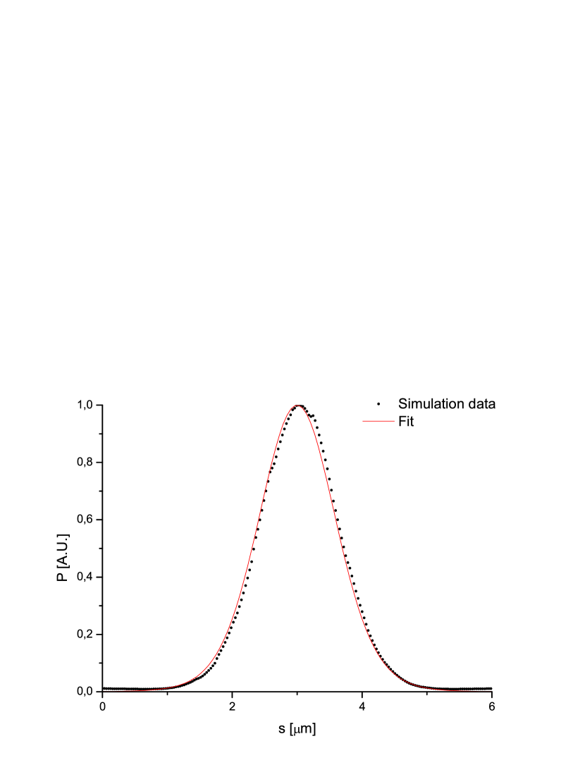
Figure 8: Normalized gain envelope after the first undulator in the case of startup from constant laser power. This plot is identical to the envelope of the average power in the case of startup from shot noise.

Since the best fit value for $\alpha$ is now fixed, we can calculate the autocorrelation trace using Eq. (5). The result is plotted with a solid line in Fig. 9. It is seen that there is a good agreement between actual intensity autocorrelation and the black circles. Deviations can be due to differences between the 1D and the 3D treatments, to the fact that in the second stage we work near to the non-linear regime, that we neglect the temporal dependence of $P_{0}$, or to the fact that for these exemplifications we used only $10$ shot averaging. However, this accuracy is sufficient for our purpose of demonstrating the feasibility of the method.

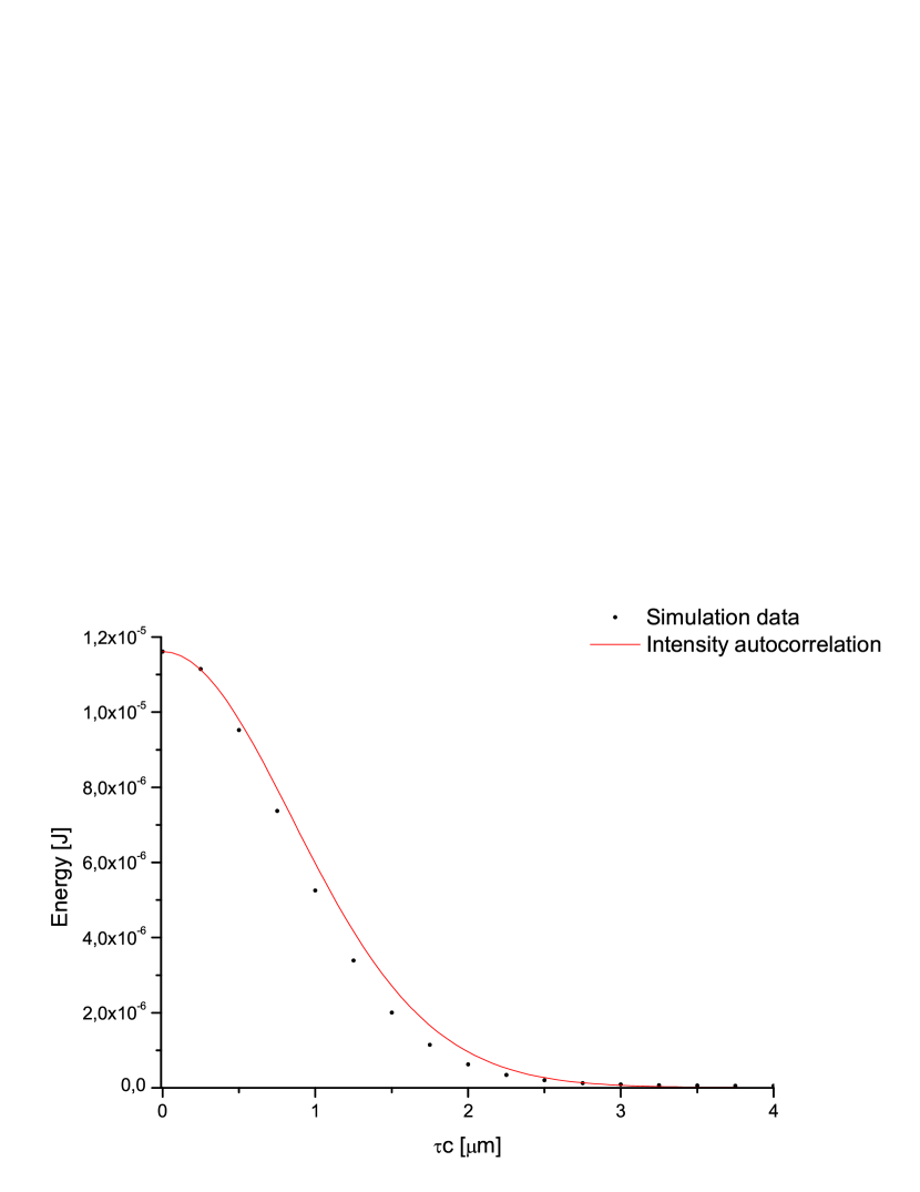
Figure 9: Energy per pulse recorded at the integrating detector as a function of the delay $\tau$. It constitutes the intensity autocorrelation trace.

Now, let us suppose that we do not know the gain curve, but we simply measure the energy per pulse from our setup, i.e. the black circles in Fig. 9. By inspecting this autocorrelation trace, we conclude that the FWHM of the autocorrelation function is about $1.9\mu$m. Assuming, as discussed above, a deconvolution factor of $1.5$, we obtain an estimate for the FWHM of the radiation pulse of about $1.3~{}\mu$m. The actual FWHM of the average power distribution from Fig. 8 is, instead, of $1.4~{}\mu$m. This gives an idea of the accuracy of the estimation of the radiation profile width with the deconvolution factor $1.5$.

3 Simplest measurement using a magnetic chicane only

As an alternative to the method considered above, we also propose a technique to measure the width of ultrafast radiation pulses based on simpler hardware. The idea is to rely on a magnetic chicane only, without an optical delay line, and is illustrated in Fig. 10. Also a magnetic chicane alone, in fact, can provide a delay of the electron beam relative to the radiation pulse, as illustrated in Fig. 11. However, the compaction factor of the magnetic chicane must always obey to the constraint to be large enough to allow for the microbunching produced in the first part of the undulator to be washed out. Therefore, the delay $\tau$ cannot be set to zero as in the previous case, and the presence of a simpler hardware is paid by the fact that the setup cannot provide a full autocorrelation trace.

Figure 10: Simplest ultra-short X-ray pulse-measurement setup which utilizes magnetic-chicane delay line only. The setup cannot provide full autocorrelation trace. The compaction factor of magnetic chicane must be large enough ( $>1\mu$m ) for performing ”fresh” bunch technique. The trace retrieval is based on computer simulations and a-priory information about electron bunch properties.

Figure 11: Sketch of X-ray intensity autocorrelation measurement using tunable magnetic delay. This autocorrelator produces part of autocorrelation trace only.

It is therefore necessary to recover the missing data with the help of computer simulations and information about the electron bunch properties, which is available from other measurements.

4 Conclusions

In this paper we presented a novel method to measure the width of ultrashort femtosecond pulses of x-rays produced in XFELs. The technique is based on the measurement of the average intensity autocorrelation function of the x-ray pulse. To this purpose, we use a fresh-bunch technique. Measurement of the energy in the radiation pulse produced in our setup yields the autocorrelation function. The method works with limited hardware, in its simplest form with a weak magnetic chicane installed in place of one of the undulator segments. The magnetic chicane can be installed without any perturbation of the XFEL focusing structure, and does not disturb the baseline undulator mode. Our proposal is therefore cheap, robust, and does not present any risk for the functionality of the facility.

5 Acknowledgements

We are grateful to Massimo Altarelli, Reinhard Brinkmann, Serguei Molodtsov and Edgar Weckert for their support and their interest during the compilation of this work.

References

- [1] G. Geloni, V. Kocharyan and E. Saldin, ”Scheme for femtosecond-resolution pump-probe experiments at XFELs with two-color ten GW-level X-ray pulses”, DESY 10-004 (2010).
- [2] G. Geloni, V. Kocharyan and E. Saldin, ”The potential for extending the spectral range accessible to the European XFEL down to 0.05 nm”, DESY 10-005 (2010).
- [3] J. Arthur et al. Linac Coherent Light Source (LCLS). Conceptual Design Report, SLAC-R593, Stanford (2002) (See also http://www-ssrl.slac.stanford.edu/lcls/cdr).
- [4] P. Emma, First lasing of the LCLS X-ray FEL at 1.5 , in Proceedings of PAC09, Vancouver, to be published in http://accelconf.web.cern.ch/AccelConf/
- [5] Y. Ding et al., Phys. Rev. Lett. 102, 254801 (2009).
- [6] M. Altarelli, et al. (Eds.) XFEL, The European X-ray Free-Electron Laser, Technical Design Report, DESY 2006-097, Hamburg (2006).
- [7] J-C. Diels and W. Rudolph, ”Ultrashort laser pulse phenomena”, AP ed. (2006)
- [8] A. Weiner, ”Ultrafast Optics”, Wiley ed., 2009
- [9] S Reiche et al., Nucl. Instr. and Meth. A 429, 243 (1999).