Differential Rotation in Fully Convective Stars

Abstract

Under the assumption of thermal wind balance and effective entropy mixing in constant rotation surfaces, the isorotational contours of the solar convective zone may be reproduced with great fidelity. Even at this early stage of development, this helioseismology fit may be used to put a lower bound on the midlatitude radial solar entropy gradient, which in good accord with standard mixing length theory. In this paper, we generalize this solar calculation to fully convective stars (and potentially planets), retaining the assumptions of thermal wind balance and effective entropy mixing in isorotational surfaces. It is found that each isorotation contour is of the form $R^{2}=A+B\Phi(r)$, where $R$ is the radius from the rotation axis, $\Phi(r)$ is the (assumed spherical) gravitational potential, and $A$ and $B$ are constant along the contour. This result is applied to simple models of fully convective stars. Both solar-like surface rotation profiles (angular velocity decreasing toward the poles) as well as “antisolar” profiles (angular velocity increasing toward the poles) are modeled; the latter bear some suggestive resemblance to numerical simulations. We also perform exploratory studies of zonal surface flows similar to those seen in Jupiter and Saturn. In addition to providing a practical framework for understanding the results of large scale numerical simulations, our findings may also prove useful in dynamical calculations for which a simple but viable model for the background rotation profile in a convecting fluid is needed. Finally, our work bears directly on an important goal of the CoRoT program: to elucidate the internal structure of rotating, convecting stars.

1 Introduction

Recent work (Balbus 2009, hereafter B09; Balbus et al. 2009, hereafter BBLW) suggests that, away from inner and outer boundary layers, the isorotation contours in the bulk of the solar convective zone (hereafter SCZ) correspond to the characteristic curves of the vorticity equation in its quasi-linear “thermal wind” form. Since both the entropy $S$ and angular velocity $\Omega$ figure in this single equation, the mathematical existence of these characteristics requires that there be some functional relationship between $S$ and $\Omega$.

B09 put forth the possibility that this relationship was a consequence of the SCZ being marginally stable to axisymmetric magnetobaroclinic modes. In BBLW, however, it was shown that an entropy/angular velocity relationship is expected to be present under very general conditions; a magnetic field is not a prerequisite. Because robust convective structures lie in surfaces in which $\Omega$ is constant, and because these structures mix entropy very efficiently, surfaces of constant entropy and surfaces of angular velocity correspond with one another. More precisely, it is not quite the entropy that is homogenized by the convective mixing, it is the “residual entropy:” some radial entropy profile must be present to trigger the convection, and it is the residual entropy, the entropy that departs from the underlying radial profile, that is homogenized by the convective mixing in constant $\Omega$ surfaces (BBLW). The confluence of constant angular velocity and constant residual entropy surfaces ensures that there is a functional relationship between them, and the existence of this functional relationship, even in the absence of knowledge of its precise form, allows one to deduce the structure of the isorotation characteristics of the thermal wind equation (hereafter TWE). If isorotational surfaces are the same as constant residual entropy surfaces, this is a result of considerable practical interest: in Appendix II, we show that it may be used in conjunction with helioseismology data to place a lower bound on the logarithmic radial entropy gradient (an otherwise observationally inaccessible quantity) of a few times $10^{-6}$. This number is good accord with mixing length theory estimates (e.g. Stix 2004).

Because the calculations presented in this paper depend strongly on the assumptions of thermal wind balance and the confluence of constant rotation and residual entropy surfaces, we review the supportive arguments that apply in environments similar to the SCZ. There are four distinct strands:

Numerical Simulations. The first piece of evidence is provided by numerical simulations. A comparison of figure (2e) (isorotational contours) and (3a) (residual entropy) in Miesch, Brun, & Toomre (2006; see also figure [2] of BBLW) shows a similarity that is striking to the eye. By way of contrast, there is no such correspondence between surfaces of total entropy and angular velocity (e.g., figure [2] in BBLW). The validity of TWB is evident in figure (5) of Miesch et al. (2006).

Dynamics. The second line of argument is based on a very simple physical picture put forth in BBLW, and has already been touched upon above. Localized, embedded disturbances in a shearing system will be distorted into surfaces of constant $\Omega$. This follows from mass conservation alone, and is most easily shown by using coordinates comoving with the background flow (BBLW). But the embedded disturbances that are of interest here are convective rolls, which mix (and thus homogenize) residual entropy. Since the convective rolls are at once in surfaces of constant rotation and constant residual entropy, these two types of surfaces must correspond.

Agreement between theory and observations. Even if a functional relationship between the angular velocity and residual entropy were simply postulated ad hoc, the resulting agreement between the calculated isorotational contours and the helioseismology data is so striking that the fit itself is an independent piece of evidence for the reasoning on which it is based (cf. fig. [1] of BBLW). The relationship traansforms the TWE from an equation relating certain partial derivatives of $\Omega$ and $S$ into a self-contained, quasi-linear partial differential equation for $\Omega$ alone. The isorotation contours then emerge as the characteristics of this equation. These characteristics thus depend for their very existence on a functional relationship between (residual) entropy and angular velocity. Without a functional relationship between entropy and angular velocity, the notion of isorotation characteristics would make no mathematical sense. With the functional relationship in place, the agreement between analytic theory and observations is remarkable.

Heuristics. A fourth line of argument depends only upon the the mathematical structure of the TWE (in its undeveloped form relating $S$ and $\Omega$) and the obeservation that the gradient of the SCZ angular velocity is dominated at mid-latitudes by its latitudinal angular component. We defer the details until the following section, when the TWE is explicitly presented.

Any of the four arguments on its own would motivate a study of convection and differential rotatation in which surfaces of constant angular velocity and constant residual entropy coincided. Taken as a whole, they comprise a truly compelling picture.

We are thus motivated to extend the mathematical technique of B09 to fully convective stars, under the assumption that solar-like dynamical conditions prevail. In practice, this means solving the TWE not just for the $1/r$ gravitational potential appropriate to the SCZ ($r$ is the usual spherical radius), but for arbitrary potentials $\Phi(r)$. We present a suite of solutions for the resulting isorotation contours under a variety of simple assumptions for the mathematical form of the entropy/angular momentum relationship as well as for the type of boundary condition used for calculating $\Omega$. We consider interior angular velocity solutions for cases in which the surface rotation is monotonically increasing from pole to equator, monotonically decreasing in the same direction, and for zonal surface flows (seen, for example, in Jupiter and Saturn) as well. We also treat problems in which the angular velocity is given along the axis of rotation, in which case there may be very little surface variation.

The profiles computed should provide a framework within which one may better understand numerical simulations of rotation in convecting stars and planets. Moreover, if the rotation profiles of at least some fully convective stars are not dominated by magnetic fields, or turbulent or meridional fluxes, the calculated isorotation contours are viable predictions for the gross interior features of these bodies. Extracting such information from the global p-mode data of fully convective stars is a primary goal of the CoRoT satellite mission.

An outline of our paper is as follows. Section 2 is a presentation of the mathematical solution for the isorotation contours of a fully convective star in which thermal wind balance is a good approximation. In section 3, we construct some specific solutions, corresponding to both solar-like and “antisolar” surface profiles, followed by models with banded zonal flows. Section 4 is a concluding discussion and summary.

2 Analysis

Throughout this paper, we follow the notation of BBLW. We denote cylindrical coordinates by radius $R$, azimuthal angle $\phi$ and axial coordinate $z$. Spherical coordinates are given by $(r,\theta,\phi)$, where $r$ is the radius from the origin, $\theta$ is the colatitude angle, and $\phi$ is once again the azimuth. Unless otherwise stated, $\Omega$, the pressure $P$ and the density $\rho$ are understood to be azimuthal averages, independent of $\phi$. The dimensionless entropy function $\sigma$ is defined by:

$$\sigma\equiv\ln P\rho^{-\gamma},$$ (1)

where $\gamma$ is the usual (specific heat ratio) adiabatic index. As noted in the Introduction, $\Phi(r)$ will refer to the local gravitational potential. For the problem of interest, $\Phi(r)$ is a well-known, tabulated function.

In thermal wind balance, one ignores contributions from convective turbulence (i.e., the convective Rossby number is small [Miesch & Toomre 2009]) and magnetic fields. This is an important simplification that appears to work well for the bulk of the convective zone of the Sun (between roughly 0.75 and 0.95 solar radii), but must of course be reexamined critically for each application.

The equation of thermal wind balance is (e.g. Thompson et al. 2003, Miesch 2005, B09):

$$R{\partial\Omega^{2}\over\partial z}=\left(1\over\gamma r\right){d\Phi\over dr}{\partial\sigma\over\partial\theta}.$$ (2)

For the SCZ, $d\Phi/dr=GM_{\odot}/r^{2}$, where $G$ is the gravitational constant and $M_{\odot}$ represents a solar mass. As in BBLW, we assume that there is a functional relationship of the form

$$\sigma^{\prime}\equiv\sigma-\sigma_{r}=f(\Omega^{2}),$$ (3)

where $\sigma_{r}$ is any function of $r$ (in practice something very close to an angle-averaged $\sigma$) and $f$ is an unspecified function. We have noted earlier that this mathematical condition will have a physical basis if convection mixes the residual entropy $\sigma^{\prime}$ in constant $\Omega$ surfaces. But the mathematical structure of equation (2) together with the most striking feature of the solar data already suggest a very simple heuristic argument (first mentioned in the Introduction) leading to a relation of the form seen in equation (3), an argument that is independent of whatever dynamical mechanism might be responsible for establishing the relationship. Helioseismology data show that at solar midlatitudes, the $\theta$ gradient of $\Omega$ dominates over its $r$ gradient. Now in the TWE, $\sigma$ is operated upon only by the $\theta$ gradient. Thus, if $\sigma$ happens to have a dominant $r$ gradient (not an unreasonable guess for the Sun), this component can largely be eliminated by subtracting off a suitably chosen radial function $\sigma_{r}$, i.e., by forming a $\sigma^{\prime}$ quantity. Substituting $\sigma^{\prime}$ for $\sigma$ does not change the TWE at all. But by its construction, this procedure will enhance the importance of the $\theta$ gradient of $\sigma^{\prime}$ relative to its $r$ gradient, and therefore it motivates a search for solutions under the assumption that $\sigma^{\prime}$ and $\Omega$ share isosurfaces in common. This is precisely the content of equation (3).

It is of interest to consider why there can be such substantial departures from the Taylor-Proudman constraint of $\Omega=\Omega(R)$ in a system that is so nearly adiabatic (and thus barotropic). The condition that isorotational and constant $\sigma^{\prime}$ surfaces coincide provides an immediate answer: if $\Omega=\Omega(R)$ then $\sigma^{\prime}=\sigma^{\prime}(R)$ and $\partial\sigma^{\prime}/\partial\theta$ must therefore be present. If this partial derivative is of order $(R\Omega/v_{s})^{2}$ or larger, where $v_{s}$ is the adiabatic sound speed, it is enough to account for the order unity departure from Taylor-Proudman columns seen in the helioseismology data and our calculations.

We assume that there is a stable, long lived average rotation profile $\Omega(r,\theta)$ that is present in the star. The evolutionary processes that are responsible for the establishment of $\Omega$ are likely to be complex, involving an as yet poorly understood combination of mechanical and thermal transport. For the problem at hand, however, these details are less important than the existence of $\Omega(r,\theta)$ itself, and the concomitant assumptions that the profile is in an average sense time steady and in thermal wind balance. If either of these assumptions fails for the fully convective stars we consider here, our model is no longer valid.

Using equation (3), the TWE (2) becomes

$${\partial\Omega^{2}\over\partial r}-\left[\left(f^{\prime}\over\gamma r^{2}\ \sin\theta\cos\theta\right){d\Phi\over dr}+{\tan\theta\over r}\right]{\partial\Omega^{2}\over\partial\theta}=0,$$ (4)

where $f^{\prime}=df/d\Omega^{2}$. The solution to equation (4) is that $\Omega^{2}$ is constant on surfaces described by

$${d\theta\over dr}=-\left(f^{\prime}\over\gamma r^{2}\ \sin\theta\cos\theta\right){d\Phi\over dr}-{\tan\theta\over r}.$$ (5)

This may be written

$${d\ \over dr}\left(r^{2}\sin^{2}\theta+{2f^{\prime}\over\gamma}\Phi(r)\right)=0,$$ (6)

which has the solution

$$r^{2}\sin^{2}\theta=A-{2f^{\prime}\over\gamma}\Phi(r),$$ (7)

where $A$ is a constant of integration. This is a rather remarkable result, and worth stating more informally: if the TWE is obeyed and entropy is mixed as efficiently as possible in constant rotation surfaces, the isorotation contours are of the form $R^{2}=A+B\Phi(r)$, where $A$ and $B$ are constants along each contour.

If our mathematical problem is to be well-posed, boundary conditions for $\Omega^{2}$ must be specified. One simple possibility is to demand that the angular velocity be a prescribed function of the colatitude angle $\theta_{0}$ on some spherical surface $r=r_{0}$. For the sake of simplicity, we consider this to be the surface of the star. Then the isorotation contour will be given by

$$r^{2}\sin^{2}\theta=r_{0}^{2}\sin^{2}\theta_{0}-{2f^{\prime}\over\gamma}[\Phi(r)-\Phi(r_{0})].$$ (8)

In some stars, however, the characteristics may be quasi-spherical, in which case most of the isorotation contours will not penetrate the surface. (This seems to be true, for example, of convective stars with a poleward increasing surface rotation rate.) We require a formulation for the characteristics that is suitable for these cases. For quasi-spherical isorotation contours, $\Omega^{2}$ is most conveniently prescribed as a function of $z_{0}$ along the axis of rotation. Then, the contours are defined by the equation

$$r^{2}\sin^{2}\theta={2f^{\prime}\over\gamma}[\Phi(z_{0})-\Phi(r)].$$ (9)

Since we will be concerned here with fully convective stars, the potential $\Phi(r)$ is that of an $n=1.5$ polytrope, where $n$ (the polytropic index) is given by $1/(\gamma-1)$. To solve for $\Phi(r)$, recall that the equation of hydrostatic equilibrium may be immediately integrated for a polytropic star, giving (e.g. Schwarzschild 1958):

$${\gamma\over\gamma-1}{P\over\rho}+\Phi(r)=-{GM\over r_{0}},$$ (10)

where $M$ is the mass of the star, and the integration constant on the right side is chosen so that the stellar potential matches the external potential $-GM/r$ at the stellar surface $r=r_{0}$. For the polytropic equation of state $P=K\rho^{\gamma}$, where $K$ is a constant defined by the adiabat, equation (10) becomes

$$(n+1)K\rho^{1/n}+\Phi(r)=-{GM\over r_{0}}.$$ (11)

To complete our determination of $\Phi(r)$, we need an explicit solution for $\rho^{1/n}$. This is given by (Chandrasekhar 1939)

$$\rho^{1/n}=\rho_{c}^{1/n}\Theta_{n}({\xi}),$$ (12)

where $\rho_{c}$ is the central density of the star, $\xi$ is the dimensionless radius

$$\xi={r\over a},\quad a^{2}={K(n+1)\rho_{c}^{(1/n)-1}\over 4\pi G}$$ (13)

and $\Theta_{n}(\xi)$ is the Lane-Emden function of order $n$, which satisfies

$${d^{2}(\xi\Theta_{n})\over d\xi^{2}}=-\xi(\Theta_{n})^{n}.$$ (14)

Extensive tables of $\Theta_{n}$ are available in the literature (e.g. Horedt 2004); for our needs a simple Padé approximant compiled by Pascual (1977) will suffice (see Appendix I).

Returning to the problem at hand, solving equation (11) for $\Phi$ now gives

$$\Phi(r)=-{GM\over r_{0}}-(5/2)K\rho_{c}^{1/n}\Theta_{3/2}(\xi).$$ (15)

The zero of $\Theta_{3/2}(\xi)$ is located at $\xi_{0}=3.65375$ (Chandrasekhar 1939), corresponding to the surface $r=r_{0}$. Our final expression for the isorotation contour (8) is given by

$$r^{2}\sin^{2}\theta=r_{0}^{2}\sin^{2}\theta_{0}+{3f^{\prime}c_{S}^{2}}\Theta_{3/2}(\xi),$$ (16)

where $c_{S}^{2}$ ($=K\rho_{c}^{1/n}$) is the square of the isothermal sound speed at the center of the star, and we have used $\gamma=5/3$. The coefficient of $\Theta_{3/2}$ will be of order $r_{0}^{2}$ if the dimensionless quantity $\Omega^{2}f^{\prime}\sim(r_{0}\Omega/c_{S})^{2}\ll 1$. The corresponding isorotation contour associated with equation (9) is

$$r^{2}\sin^{2}\theta={3f^{\prime}c_{S}^{2}}[\Theta_{3/2}(\xi)-\Theta_{3/2}(z_{0}\xi_{0}/r_{0})],$$ (17)

where $z_{0}$ refers to the value of $z$ at the start of the characteristic along the axis of rotation. The ratio $z_{0}/r_{0}$ thus runs between $0$ and $1$.

For solar-like surface profiles, $f^{\prime}$ will generally be negative. This is because convection is more efficient along the rotation axis, so the poles will be associated with higher temperatures and small rotation rates relative to the equator. For antisolar profiles, similar reasoning suggests that $f^{\prime}$ should be positive. It is not yet possible to say more than this without detailed numerical simulations of the turbulent flow in convective stars. In the spirit of B09 and BBLW, we therefore introduce the function $F(\sin^{2}\theta_{0})$, which is of orer unity, rewriting equation (16) as

$$(r/r_{0})^{2}\sin^{2}\theta=(\xi/\xi_{0})^{2}\sin^{2}\theta=\sin^{2}\theta_{0}+F(\sin^{2}\theta_{0})\Theta_{3/2}(\xi),$$ (18)

where

$$F(\sin^{2}\theta_{0})\equiv{3f^{\prime}c_{S}^{2}\over r_{0}^{2}}<0$$ (19)

is some simple dimensionless function of $\sin^{2}\theta_{0}$. In practice, we will limit ourselves to linear or constant functions, there being at this stage no particular exigency for greater mathematical sophistication.

For solar-like surface profiles, let us assume that $F(\sin^{2}\theta_{0})=-\beta_{1}-\beta_{2}\sin^{2}\theta_{0}$. Then, solving for $\sin^{2}\theta_{0}$ leads to

$$\sin^{2}\theta_{0}={(\xi/\xi_{0})^{2}\sin^{2}\theta+\beta_{1}\Theta_{3/2}(\xi)\over 1-\beta_{2}\Theta_{3/2}(\xi)}.$$ (20)

If $\Omega^{2}$ is now a specified function at the surface, $\Omega_{0}^{2}(\sin^{2}\theta_{0})$ say, the solution throughout the stellar interior is given by substituting for $\sin^{2}\theta_{0}$ from equation (20) in the argument of $\Omega_{0}^{2}$. This is the desired solution when $\Omega_{0}$ is specified initially on a spherical surface.

For the antisolar surface profiles, the $z_{0}$ inversion associated with equation (17) is somewhat complicated, except when $F$ is a (positive) constant, and we will restrict ourselves in this work to this case. We then find

$$\left(z_{0}\xi_{0}\over r_{0}\right)^{2}=\Lambda(X),\quad X\equiv\Theta_{3/2}(\xi)-{\xi^{2}\over\xi_{0}^{2}F}\sin^{2}\theta,$$ (21)

where the (very simple) $\Lambda$ function, essentially an inversion of $\Theta_{3/2}$, is presented in Appendix I. Given the rotation profile along $z_{0}$, $\Omega_{0}^{2}(z_{0}^{2})$ say, the solution throughout the stellar interior is given by substituting for $z_{0}^{2}$ from equation (21) in the argument of $\Omega_{0}^{2}$.

3 Contour description

3.1 Solar surface profiles

We choose the surface rotation profile $\Omega(\sin^{2}\theta_{0})$ to be equal to be that of the Sun, a simple Taylor expansion in $\sin^{2}\theta_{0}$:

$$(\Omega_{0}/2\pi)=(386.2+198.7\sin^{2}\theta_{0}-66.7\sin^{4}\theta_{0}).$$ (22)

The units on the right are nano-Hz. Representative solutions are shown in figures 1–4.

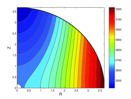
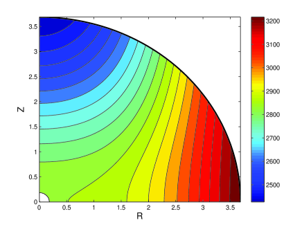
Figure 1: Isorotation contours for a solar surface rotation profile. In all figures, the abscissa $R$ and ordinate $Z$ are given in units of the Lane-Emden radius $a$ (eq. [13]). $\beta_{1}=0.2$, $\beta_{2}=0$ (left); $\beta_{1}=0.4$, $\beta_{2}=0.0$ (right).

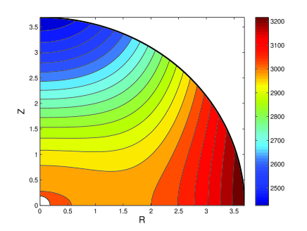
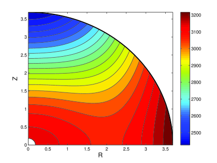
Figure 2: As in figure(1), with $\beta_{1}=0.6$, $\beta_{2}=0.0$ (left); $\beta_{1}=0.8$, $\beta_{2}=0.0$ (right).

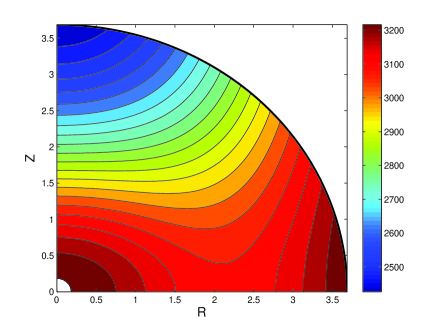
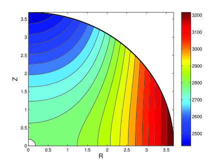
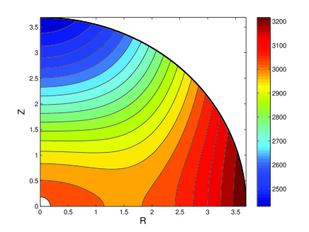
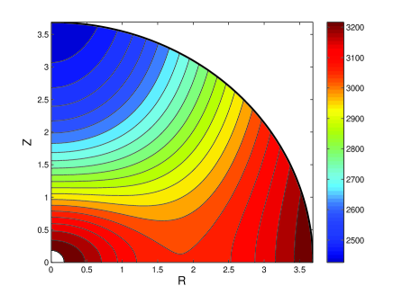
Figure 3: As in figure (1), with $\beta_{1}=0.5$, $\beta_{2}=0.5$ (left); $\beta_{1}=0.5$, $\beta_{2}=-0.5$ (right).

Figure 4: As in figure (1), with $\beta_{1}=0.5$, $\beta_{2}=0.2$ (left); $\beta_{1}=0.2$, $\beta_{2}=0.8$ (right).

The four profiles of figures 1 and 2 correspond to a suite of increasing values of $\beta_{1}$, $(0.2,0.4,0.6,0.8)$ that show the contours evolving from nearly cylindrical Taylor-Proudman columns (corresponding to the limit $\beta_{1}=\beta_{2}=0$), to a much more “flat-bottomed” configuration. In figures 3 and 4, we allow $\beta_{1}$ and $\beta_{2}$ to vary separately, as indicated in the captions. Aside from a tightening or loosening of the contours, there is not a great qualitative difference between the cases of vanishing versus finite $\beta_{2}$.

The isorotation contours are, roughly speaking, divided into two classes, which we will term polar and equatorial. Polar contours extend from the surface, and cross through the rotation axis. Equatorial contours, by contrast, extend from the surface and cross through the equatorial plane. In some cases, there are contours that remain within the star, never reaching the surface. These tend to be quasi-spherical, deep in the interior near the stellar core. Mathematically, this corresponds to values of $\sin^{2}\theta_{0}$ in excess of unity, but the contours themselves are not unphysical: they simply remain below the surface of the star, and are valid solutions of the TWE.

There is a particular value for $\theta_{0}$, say $\theta_{c}$, which is the critical divide. Contours with $\theta_{0}<\theta_{c}$ are polar, while contours with $\theta_{0}>\theta_{c}$ are equatorial. In no cases do contours cross: caustics are absent from the solutions that we have studied. This is not true for the $1/r$ potential used in the calculations of B09 and BBLW. In that case, caustics formed when the solutions were extended beneath the convection zone. The Lane-Emden function $\Phi_{3/2}(\xi)$, on the other hand, is evidently sufficiently well-behaved at small $r$ to avoid the formation of caustics in the isorotation contours.

Perhaps the most striking feature of these plots is how reminiscent of the Sun they are, despite the different gravitational potential and the extended domain. The contours show the familiar basic pattern of lying in planes of constant $z$ near the axis of rotation, becoming much more cylindrical near the equator, and quasi-radial in the transition region between. Closer to the stellar surface, we see the characteristic solar feature of parallel lines once again in evidence. We have of course chosen a solar-like surface profile, but the results are generic for any slowly varying, poleward decreasing, surface profile with reflection symmetry about the equator.

3.2 Antisolar surface profiles.

We next relax the constraint of a poleward decreasing surface rotation profile. Poleward increasing profiles are seen in simulations of convective red giant stars (Brun & Palacios 2009). Since thermal convection is expected still to be most efficient parallel to the rotation axis (where it is unencumbered by the Coriolis force), the function $f^{\prime}(\Omega^{2})$ is now negative. This causes interesting changes in the geometry of the isorotation contours.

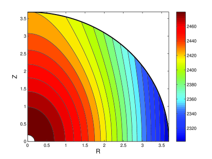
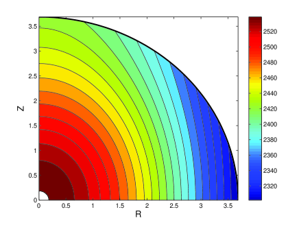
Figure 5: Isorotation contours for an antisolar surface rotation profile (eq. [23]). As in figure (1), the abscissa $R$ and ordinate $Z$ are given in units of the Lane-Emden radius $a$ (eq. [13]). $\beta_{1}=-0.5$, $\beta_{2}=0$ (left); $\beta_{1}=-1.0$, $\beta_{2}=0.0$ (right).

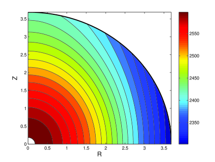
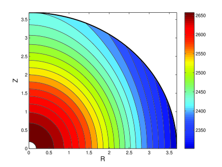
Figure 6: As in figure (5), with $\beta_{1}=-1.5$, $\beta_{2}=0.0$ (left); $\beta_{1}=-2.0$, $\beta_{2}=0.0$ (right).

3.2.1 $\Omega$ initially specified on the surface

Figures (5) and (6) show a suite of internal isorotation contour diagrams for a poleward increasing surface profile:

$$(\Omega/2\pi)=386.2-19.87\sin^{2}\theta_{0}.$$ (23)

Compared with equation (22) for our fiducial solar poleward decreasing profile, we have changed the sign of the $\sin^{2}\theta_{0}$ term and reduced its magnitude by a factor of ten. We display four values of $\beta_{1}$, $-0.5,-1,-1.5,-2$, with $\beta_{2}$ set equal to $zero$, so that $f^{\prime}$ is a global constant. The isorotation contours in this case do not resemble the Sun at all, for they now have a different topology. There is, for example, no critical contour dividing isorotation curves that start at the surface and then head either for the axis or for the equator. Instead, all contours cross the equatorial plane, and curve in the same sense (toward the rotation axis) as they rise upward from the equator. The most strongly inwardly curving contours first find the rotation axis (where they end), the less strongly curved contours encounter the surface before the axis. This is reminscent of the slowly rotating red giants in the Brun & Palacios (2009) simulations. In the numerical studies, however, the surface is in near uniform rotation and is best approached using the formalism of equation (9) (see below). For small values of $|\beta_{1}|$, the contours look, not surprisingly, cylindrical. This is clearly the Taylor-Proudman regime. But as the magnitude of $\beta_{1}$ increases, the contours become more spherical (prolate). In contrast to the case of solar surface profiles (and the Sun itself), in which the rotation rate increases with distance from the axis, the antisolar surface profiles are associated with an interior rotation structure with $d\Omega^{2}/dR<0$.

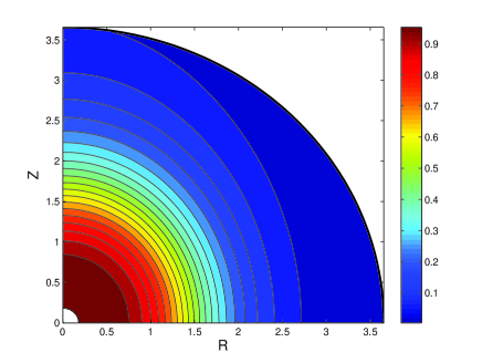
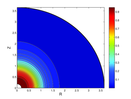
Figure 7: Internal isorotation contours for a convective star with $\Omega$ specified along the rotation axis. The solution is generated by equations (17), (21), and (24). The abscissa $R$ and ordinate $Z$ are given in units of the Lane-Emden radius $a$ (eq. [13]). $F=2$ and $\beta=0.1$ (left) and $1$ (right).

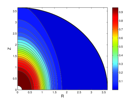
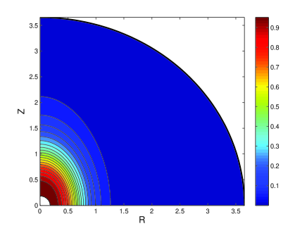
Figure 8: As in figure (7), with $F=0.4$, $\beta=0.1$ (left), $\beta=1$ (right).

3.2.2 $\Omega$ initially specified along the rotation axis

In stars showing significantly more $\Omega$ variation along the axis of rotation than along a surface meridional contour, it makes sense to consider the initial rotation function to be of the form $\Omega_{0}(z_{0}^{2})$, and use the formulation embodied in equations (17) and (21). We have adopted the model

$$\Omega_{0}(z_{0}^{2})=\left[1+\beta z_{0}^{4}\right]^{-1},$$ (24)

leaving $\beta$ as a parameter. Specifying the function $F$ (treated here as a constant) and $\beta$ then uniquely defines the model.

Figures (7) and (8) show a selection of results. In figure (7), we have set $F=2$. On the left, $\beta=0.1$; on the right, $\beta=1$. In figure (8), $F=0.4$ with $\beta=0.1$ on the left and $\beta=1$ on the right. The larger value of $F$ in figure (7) corresponds to a smaller rotation rate, and the isorotation contours are more rounded. Figure (8) corresponds to a larger rotation rate, and the contours are more elongated along the axis, distorted in the direction of Taylor-Proudman columns. Depending on the value of $\beta$, the rotation can either be confined to a central core or extend to the surface. These findings compare very favorably with the morphologies found in the numerical simulations of Brun & Palacios (2009).

3.3 Zonal surface flows

Going further afield, one may speculate on what our theory would predict for the internal rotation profile of a convecting body whose surface exhibited zonal flow—as is seen in the giant planets of our solar system. This truly is a speculative domain, since even the sign of the $d\sigma^{\prime}/d\Omega^{2}$ is not certain for this class of flows. Our motivation is simply to note an alternative to Taylor-Proudman columns for the internal flow contours of giant convecting gaseous planets and possibly brown dwarfs. In the case of Jupiter and Saturn the surface flows are likely to be shallow (e.g., Liu, Goldreich, & Stevenson 2008), and it is not known whether the convective interior supports such banded streams. Thus, whereas the solar problem is tightly confined, and the deep convective envelope with a monotonic surface rotation profile is at least a well-motivated problem, this particular application is truly “untethered.” These are purely formal solutions to the TWE.

We consider a surface profile of the form

$$\Omega_{0}={\rm Const.}+\sin(4\pi\sin^{2}\theta_{0}).$$ (25)

In figures 9 and 10, we show a suite of four representative results with the equation (20) parameters, $\beta_{1}=0.2,0.4,0.6,0.8$ and $\beta_{2}=0$. As $\beta_{1}$ increases, the departure of the isorotation contours from Taylor-Proudman columns is evident, until by $\beta_{1}=0.8$ many contours show relatively little variation in $y$. Closer to the equator, however, the contours retain their cylindrical form. As noted in BBLW, rapid rotators are probably characterized by relatively small $\beta_{1}$, because of the $1/\Omega^{2}$ scaling of $f^{\prime}(\Omega^{2})$.

These results can be compared with numerical simulations of convectively driven differential rotation in Jupiter, Saturn, Uranus and Neptune. Such models have grown progressively more realistic, moving from mean-field (Rieutord et al.  1984) to Boussinesq (e.g Aurnou & Heimpel 2004; Aurnou, Heimpel & Wicht 2007), and most recently to anelastic (Jones & Kuzanyan 2009) approximations. In the latter calculations, the Taylor-Proudman constraint is dominant, and the zonal velocity tends accordingly to be constant on cylinders.

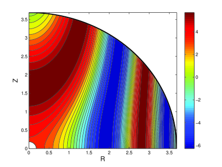
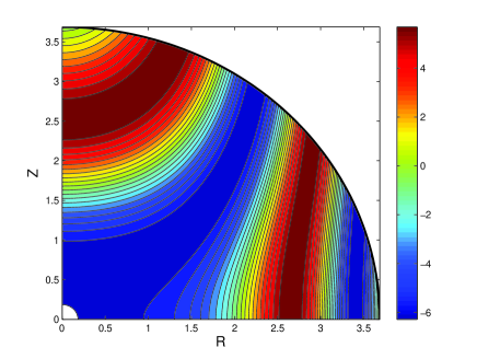
Figure 9: Banded surface profile given by equation (25). The abscissa $R$ and ordinate $Z$ are given in units of the Lane-Emden radius $a$ (eq. [13]). $\beta_{1}=0.2$, $\beta_{2}=0$ (left); $\beta_{1}=0.4$, $\beta_{2}=0.0$ (right).

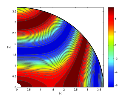
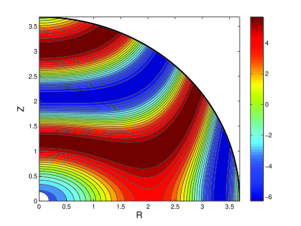
Figure 10: As in figure (9), with $\beta_{1}=0.6$, $\beta_{2}=0.0$ (left); $\beta_{1}=0.8$, $\beta_{2}=0.0$ (right).

4 Discussion

Our principal result, embodied in equation (7), is one of remarkable simplicity. If, in a convecting star, thermal wind balance holds and entropy is well mixed in surfaces of constant angular velocity, the form of the constant $\Omega$ surface passing through a point in the $r$, $\theta$ plane depends only upon the gravitational potential and a single “adjustable” constant. This constant is, in principle, determined from fundamental dynamics, but in practice it depends upon knowing how to treat the details of convective turbulent transport. One of the important consequences of this work, however, is precisely this point: ignorance of the details of turbulent transport does not mean complete ignorance of the consequences of the transport—in this case, the shapes of the isorotation surfaces.

Unfortunately, unlike helioseismology, the fields of astero- and planetary seismology are still very much in their infancies. There are no data of quality comparable to the solar results with which we may compare our computed profiles. Until such data are available, the practical utility of our results will primarily be as an aid for understanding numerical simulations, and for theoretical investigations of convective processes in which a average equilibrium rotation needs to be specified or understood (e.g. stellar evolution and dynamo theories).

In principle, large scale numerical computations of fully convective stars are amenable to development at a level evinced by the solar convection studies (see, e.g. Miesch & Toomre 2009). But in practice, this class of calculation is extremely demanding of resources, so that only the SCZ has been explored in detail and under a large variety of physical assumptions. Recent work, however, has shown that numerical simulations of convective envelopes are viable, and properly interpreted, a potentially rich source of dynamical information (e.g. Browning 2008; Brun & Palacios 2009 and references therein). The investigation of Brun & Palacios (2009) centered on four models of red giant stars. The more slowly rotating envelopes produced quasi-spherical shells for the isorotational surfaces, while the more rapidly rotating models showed classic Taylor-Proudman cylinders. Our calculations also show this trend; indeed, strikingly so. More troublesome, for a direct application of the work presented in the current paper, is the fact that our assumption of thermal wind balance was not a particularly accurate approximation to the vorticity equation in the simulations: both turbulent fluctuations and meridional circulation appeared to be more important in the red giant calculations than in the numerical simulations of the SCZ. Neither is convective Rossby number small for the simulations, as it is for the Sun. Yet the gross features of the red giant simulations seem rather well captured by our approach, and this is not because the models lack predictive power: inapproprately changing the sign of $F$, for example, destroys even the qualitative agreement with simulations in both the solar and red giant studies. Thus the marginality of our assumptions in the case of the latter may be more of a technical concern than a real conceptual impediment for understanding the qualitative structure of the flow. But clearly much more can be done.

Another issue that we have not touched on is the effect of magnetic fields, shown in an extreme form by Browning’s (2008) model of a fully convective M-star, where magnetic stresses transform a cylindrical $\Omega$-profile into almost uniform rotation. There is in fact an interesting analogy between the roles of residual entropy and of magnetic fields in coupling differentially rotating cylinders (Taylor 1963; Fearn 2007).

Unlike the compelling fit of the solar isorotational contours presented in BBLW, the results presented in the current work must wait before observational comparisons are possible. Comparison with simulations is encouraging, however, and shows promise of genuine progress on both the analytic and numerical fronts. In it is particularly noteworthy, for example, that the poleward-increasing rotation profiles associated with at least some classes of fully convective stars show concave internal isorotation contours in simulations. We are in the early days yet of a field that is both rapidly and fruitfully developing. Even if only a small class of fully convective systems has isorotation contours described by equation (7), this would be extremely useful. Not only would a piece of stellar hydrodynamics be secured, but a point of departure for more complex conditions would be established.

Appendix I: Padé approximants for $\Theta_{3/2}(\xi)$.

For the calculations presented in this paper, we have adopted the following Padé approximant for the $n=3/2$ Lane-Emden function $\Theta_{3/2}(\xi)$ (Pascual 1977):

$$\Theta_{3/2}(\xi)\simeq{1-a_{1}\xi^{2}+a_{2}\xi^{4}\over 1+b_{1}\xi^{2}+b_{2}\xi^{4}},$$ (26)

where

$$a_{1}=8.46561\times 10^{-2},\qquad a_{2}=8.156966\times 10^{-4},$$ (27)

and

$$b_{1}=8.201058\times 10^{-2},\qquad b_{2}=1.984127\times 10^{-3}.$$ (28)

A simpler, and only slightly less accurate approximation is given by

$$\Theta_{3/2}(\xi)\simeq{1-a\xi^{2}\over 1+b\xi^{2}},$$ (29)

where

$$a=7.490699\times 10^{-2},\qquad b=9.175968\times 10^{-2}.$$ (30)

The $a$ and $b$ constants are chosen so that the rational function goes to zero precisely at $\xi=\xi_{0}=3.65375$, and to $1-\xi^{2}/6$ for small $\xi$. Contour plots produced by this approximation are almost indistinguishable from those shown in the paper. An advantage of this form for $\Theta_{3/2}(\xi)$ is that it is easily invertible:

$$\xi^{2}={1-\Theta\over a+b\Theta}\equiv\Lambda(\Theta),$$ (31)

a desirable quality in some applications. (We have suppressed the subscript $3/2$ on $\Theta$ for clarity of presentation.) This defines the $\Lambda$ function used in equation (21).

Appendix II: Residual entropy bound

The mathematical identity

$$\left(\partial\sigma^{\prime}\over\partial r\right)_{\theta}=-\left(\partial\theta\over\partial\ln r\right)_{\sigma^{\prime}}\left({1\over r}{\partial\sigma^{\prime}\over\partial\theta}\right)_{r}$$ (32)

may be used to establish a lower limit to the radial entropy gradient in the SCZ. Following the notion that constant $\sigma^{\prime}$ and constant $\Omega$ surfaces coincide, the first partial derivative on the right side of the equation may be read off directly from the helioseismology data. The second partial derivative on the right is evaluated via the TWE. The result is

$$\left(\partial\sigma^{\prime}\over\partial\ln r\right)_{\theta}=-2\gamma\tan\theta\left(\partial\ln\Omega\over\partial\ln z\right)_{R}\left(\partial\theta\over\partial\ln r\right)_{\sigma^{\prime}}\left(r\Omega^{2}\over g\right),$$ (33)

where $g$ is the gravitational field of the SCZ, taken here to be $2.74\times 10^{4}$ cm² s^-1. Using recent GONG data (kindly supplied to us by R. Howe), we estimate the logarithmic $\Omega$ derivative as $-0.12$ and the $\theta$-$\ln r$ gradient as $-0.3$. Then with $r=5.95\times 10^{10}$ cm (or 0.85 solar radii), $\Omega=2.5\times 10^{-6}$ s^-1, and $\gamma=1.67$, we obtain

$$\left(\partial\sigma^{\prime}\over\partial\ln r\right)_{\theta}=-1.6\times 10^{-6}\tan\theta.$$ (34)

The numerical values correspond to regions of the SCZ near $\tan\theta=1$. Since $\sigma=\sigma^{\prime}+\sigma_{r}$, this number is likely to be a lower bound (in magnitude) to the true midlatitude solar radial entropy gradient $\partial\sigma/\partial\ln r$. Mixing length theory gives values between $10^{-6}$ and $10^{-5}$ for the absolute value of this gradient (e.g. Stix 2004).

References

- Aurnou et al. (2004) Aurnou, J. M. & Heimpel, M. 2004, Icarus, 169, 492
- Aurnou et al. (2007) Aurnou, J. M., Heimpel, M. & Wicht, J. 2007, Icarus, 190, 110
- Balbus (2009) Balbus, S. A., 2009, MNRAS, 395, 2056 (B09)
- Balbus et al. (2009) Balbus, S. A., Bonart, J., Latter, H., & Weiss, N. O. 2009, MNRAS, 400, 176 (BBLW)
- Browning (2008) Browning, M. 2008, MNRAS, 676, 1262
- Brun et al. (2009) Brun. A. S., Antia, H. M., & Chitre, S. M. 2009, ariXive:0910.4954v1 [astro-ph.SR]
- Brun & Palacios (2009) Brun, A. S., & Palacios, A. 2009, ApJ, 702, 1078
- Chandrasekhar (1939) Chandrasekhar, S. 1939, Theory of Stellar Structure (New York: Dover)
- Fearn (2007) Fearn, D. R. 2007, In “Mathematical Aspects of Natural Dynamos”, eds. E. Dormy & A. M. Soward (Boca Raton: Grenoble Sciences/CRC Press), p. 201
- Horedt (2004) Horedt, G. P. 2004, Polytropes: Applications in Astrophysics and Related Fields (Dordrecht: Kluwer)
- Jones & Kuzanyan (2009) Jones, C. A. & Kuzanyan, K. 2009, Icarus, 204, 227
- Liu et al. (2008) Liu, J., Goldreich, P. M., & Stevenson D. J. 2008, Icarus, 196, 653
- Miesch (2005) Miesch. M. 2005, Living Revs. Sol. Phys., 2, 1 (www.livingreviews.org/lrsp-2005-1)
- Miesch et al. (2006) Miesch, M. S., Brun, A. S., Toomre, J. 2006, ApJ, 641, 618
- Miesch & Toomre (2009) Miesch, M. S., & Toomre, J. 2009, Ann. Rev. Fluid Mech., 41, 317
- Pascual (1977) Pascual, P. 1977, A&A, 60, 161
- Rieutord et al. (1994) Rieutord, M., Brandenburg, A., Mangeney, A. & Drossart, P. 1994, A&A, 286, 471
- Schwarzschild (1958) Schwarzschild, M. 1958, Structure and Evolution of the Stars (New York: Dover)
- Stix (2004) Stix, M. 2004, The Sun: An Introduction (Berlin: Springer-Verlag)
- Taylor (1963) Taylor, J. B. 1963, Proc. Roy. Soc. A, 274, 274
- Thompson (2003) Thompson, M. J., Christensen-Dalsgaard, J., Miesch, M. S., & Toomre, J. 2003, ARAA, 41, 599