Fractal design for an efficient shell strut under gentle compressive loading

Abstract

Because of Euler buckling, a simple strut of length $L$ and Young modulus $Y$ requires a volume of material proportional to $L^{3}f^{1/2}$ in order to support a compressive force $F$, where $f=F/YL^{2}$ and $f\ll 1$. By taking into account both Euler and local buckling, we provide a hierarchical design for such a strut consisting of intersecting curved shells, which requires a volume of material proportional to the much smaller quantity $L^{3}f\exp\left[2\sqrt{(\ln 3)(\ln f^{-1})}\right]$.

I Introduction

Fractals Mandelbrot occur ubiquitously in nature and appear to arise in many different ways; examples from the physical and biological sciences include colloidal flocculationLin ; Kantor , percolation phenomenaIsichenko and the structure of transport networks in organismsWest . In the area of structural mechanics, it has been claimed that the fractal morphology of trabecular bone is responsible in part for its mechanical efficiency Huiskes1 ; while the complex suture patterns of ammonites of the Jurassic and Cretaceous periods have been conjectured to give greater strength to their shellsJacobs ; Batt .

Recent theoretical work on a highly simplified model system consisting of a brittle pressure-bearing plate has also suggested that a fractal structure can be highly efficient when the loading conditions are very gentle and the material very brittle Farr . It is therefore of interest to explore other circumstances under which fractal design principles can lead to high mechanical efficiency, in case there is a general theorem underlying the optimal design of elastic structures under gentle compressive loading. To this end, we consider here the buckling behaviour of compression members.

Consider first the classical case of an Euler strut Euler in the form of a solid, cylindrical column of radius $r_{0}$ and length $L$, made from an isotropic, linear elastic material of Young modulus $Y$ and Poisson ratio $\nu$, and subject to a compressive force $F$ at the freely hinged ends.

We define two non-dimensional parameters: $f\equiv F/(YL^{2})$, which is the compressive force scaled by $YL^{2}$, and $v=\pi r_{0}^{2}/L^{2}$, which is the volume of material used, scaled by $L^{3}$. We are interested in the regime of gentle loading, by which we mean $f\ll 1$ and $v\ll 1$.

Because of Euler buckling, the strut can only withstand forces such that $F<\pi^{2}YI_{0}/L^{2}$, where $I_{0}=\pi r_{0}^{4}/4$ is the second moment of the cross sectional area about the neutral axis of the beam Euler ; Timoshenko . Therefore the (non-dimensionalised) volume of material required to withstand a load represented by $f$ is given by

$$v(0)=2\pi^{-1/2}f^{1/2},$$ (1)

where we have neglected the material required to make the freely hinged couplings at the ends of the strut. For the purposes of this paper, we call the above solid strut a “generation $G=0$” structure, and this is written as an argument for the volume variable $v$ in Eq. (1).

We note in passing that the contrast in efficiency between compression members and tension members (for which $v\propto f$) is a persistent theme in structural engineering. The scaling of Eq. (1) plus the cost of couplings mean that efficient structures tend to have few compression members and many long tension members; the paradigmatic example being a tent Cox ; Gordon .

To define a $G=1$ structure, we choose a hollow cylindrical shell, which is also a classic problem in elasticity theory Timoshenko ; Koiter . We choose the length as always to be $L$, and we denote the radius by $r_{1,1}$ where the first index refers to the “generation number” $G=1$ and the second index will be explained when we describe structures of higher generation number. This $G=1$ structure consists of one cylinder parallel to the compression direction, and we express this trivial fact by $n_{1,1}=1$. The thickness of the sheet of elastic material making up the curved surface of the cylindrical shell is denoted by $s_{1,1}$, which specifically represents the volume of material required to make unit area of the curved surface. We call this quantity the “material thickness” of the curved sheet. We also introduce an “effective elastic thickness” $t_{1,1}$ for the curved sheet. For the generation 1 structure, the curved sheet is simple in topology and uniform in thickness, and so $s_{1,1}\equiv t_{1,1}$. Lastly we have an effective Young modulus $Y_{1,1}$ and Poisson ratio $\nu_{1,1}$ for the sheet. For a $G=1$ structure $Y_{1,1}\equiv Y$ and $\nu_{1,1}\equiv\nu$. In all of these expressions, the first index refers to the generation number, and the second index will take values from $1$ up to the generation number of the structure, as will be explained in section III.

Provided that $t_{1,1}\ll r_{1,1}\ll L$, the column now has a second moment of cross sectional area about the neutral axis given by $I_{1}=\pi s_{1,1}r_{1,1}^{3}$ and the volume of material used to construct it is given by $v=2\pi r_{1,1}s_{1,1}/L^{2}$. The requirement that Euler buckling not occur then imposes the constraint $F<\pi^{2}Y_{1,1}I_{1}/L^{2}$ or

$$v>2f^{1/3}\left(t_{1,1}/L\right)^{2/3}.$$ (2)

In contrast to the solid column, there is now the possibility of local buckling. This happens when Koiter ; Timoshenko

$$F=\frac{2\pi Y_{1,1}t_{1,1}^{2}}{\sqrt{3(1-\nu_{1,1}^{2})}},$$ (3)

which provides a second constraint on the structure required to support a force $F$.

The generation $1$ structure with the highest mechanical efficiency (smallest value of $v$ for a given $f$) is therefore specified by:

$$v(1)=2\left[\frac{3(1-\nu^{2})}{4\pi^{2}}\right]^{1/6}f^{2/3}$$ (4)

with

$$\frac{r_{1,1}}{L}=\frac{1}{\pi}\left[\frac{3(1-\nu^{2})}{4\pi^{2}}\right]^{-1/12}f^{1/6},$$ (5)

$$\frac{t_{1,1}}{L}=\left[\frac{3(1-\nu^{2})}{4\pi^{2}}\right]^{1/4}f^{1/2}$$ (6)

and therefore $t_{1,1}\ll r_{1,1}\ll L$ as assumed above.

Eq. (4) represents a considerable gain in efficiency over the solid column of Eq. (1), but does not rival the efficiency ($v\propto f$) which can be obtained for tensile loading.

We note that both here and in all subsequent sections, we have taken a conservative approach in calculating $v$, by assuming that the structure fails when the first buckling bifurcation is encountered. Engineering structures (especially shells) will often support considerably higher loads in the post-buckling regime before catastrophic failure Timoshenko . Although such complexities are certainly of practical importance, we choose to ignore them in this investigation and try, where possible, to obtain estimates which are upper bounds for $v$.

II A composite plate

When designing a plate or shell which may buckle, it is standard engineering practice to introduce stiffening plates, longitudinal stringers, bulkheads, or similar devices in order to stiffen the structure and/or suppress buckling modes Timoshenko ; Gordon .

In this paper we take a similar approach, but re-design the structure in a systematic and hierarchical manner, which can be iterated in the limit $f\rightarrow 0$. We do not presume to do this in the most efficient manner (we are almost certainly over-engineering the protection against many of the buckling modes we wish to avoid) but nevertheless the design we describe allows us to systematically change the scaling of $v$ with $f$ and therefore to approach more closely the scaling which can be achieved for a rod under tension; achieving ultimately $v\propto f\exp\left[2\sqrt{(\ln 3)(\ln f^{-1})}\right]$. In the limit $f\rightarrow 0$, this is smaller than any scaling of the form $v\propto f^{\beta}$ with $\beta<1$.

To proceed in this direction, consider first of all a simple thin, flat plate of uniform thickness $\tilde{t}$, lying in the $x-y$ plane and made out of an isotropic elastic material of Young modulus $\tilde{Y}$ and Poisson ratio $\tilde{\nu}$. Suppose furthermore that this plate may be deformed by applied stresses, leading to stretching or shearing of the middle planeTimoshenko2 , and also possibly to out-of-plane deflections which may be large compared to the plate thickness. An appropriate approximation to describe the behaviour of the plate is due to von Karman vonKarman . In this theory, the equilibrium behaviour (given suitable boundary conditions) can be obtained by minimising an energy functional. The elastic part of the energy (as opposed to that from external forces) can be written as the sum of two terms Lobkovsky : the energy $U_{S}$ associated with stretching of the middle plane of the plate, and a bending energy $U_{B}$.

If the 2-dimensional strain tensor for the middle plane of the plate is given by ${\rm e}(x,y)$, then the stretching energy will be given by Timoshenko ; Lobkovsky ; Farr

$$U_{S}=\frac{\tilde{Y}\tilde{t}}{2(1-\tilde{\nu}^{2})}\int dxdy\left\{\tilde{\nu}\left[{\rm Tr}({\rm e})\right]^{2}+(1-\tilde{\nu}){\rm Tr}({\rm e}^{2})\right\}.$$ (7)

Furthermore, if the plate is bent out-of-plane in the $z$-direction, by an amount $w(x,y)$, then the bending energy stored will be given by Lobkovsky

$$U_{B}=\frac{\tilde{Y}\tilde{t}^{3}}{24(1-\tilde{\nu}^{2})}\int dxdy\left\{\left[{\rm Tr}(H)\right]^{2}-2(1-\tilde{\nu}){\rm det}(H)\right\},$$ (8)

where $H$ is the Hessian matrix

$$H(x,y)=\left(\begin{array}[]{cc}\frac{\partial^{2}w}{\partial x^{2}}&\frac{\partial^{2}w}{\partial x\partial y}\\ \frac{\partial^{2}w}{\partial x\partial y}&\frac{\partial^{2}w}{\partial y^{2}}\end{array}\right).$$ (9)

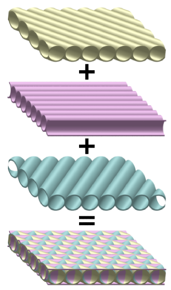
Figure 1: Bottom image is part of a composite plate, which is constructed by merging the three substructures shown in the top three images of the figure. Each substructure is an infinite set of parallel right circular cylinders which are joined along their lines of osculation. The three sub-structures are identical save for being rotated by $\pm 2\pi/3$ radians relative to one another about an axis perpendicular to the plane. Each right circular cylinder has a radius $r$, a wall thickness $t\ll r$ and is infinitely long.

Now consider the composite plate shown in the bottom part of Fig. 1. This structure is built from three intersecting sub-structures (as shown separately in the top three parts of Fig. 1), each identical, save for being rotated $\pm 2\pi/3$ radians relative to one another. Where the sub-structures pass through one another, we imagine them being joined or welded along their curves of intersection. Each sub-structure consists of an infinite set of parallel hollow right circular cylinders, with their axes in the $x-y$ plane, and placed so that each touches two neighbours and is welded to each of its two neighbours along these lines of contact (which also lie in the $x-y$ plane). We specify all these welds so we can be sure that on deformation at long length scales, the plate behaves as a single entity, rather than separating into its constituent cylinders.

Each of the component cylinders has a radius $r$ and a wall thickness $t\ll r$. Because we have chosen the composite plate to have six-fold rotational symmetry about the $z$-axis, then on long enough length scales the composite plate must behave elastically as though it is isotropic under rotations about the $z$-axis. This is because to leading order, the elastic stiffness of the plate under stretching and bending is represented by rank 4 tensors in two dimensions (which are contracted with two dimensional rank 2 deformation tensors to form the scalar energy). These rank 4 elastic tensors may be invariant under rotation about the $z$-axis (and so be consistent with any rotation group $C_{n}$), or may have one of the symmetry groups $C_{2}$ or $C_{4}$. However the composite plate we have described has the symmetry group $C_{6}$, which is not consistent with $C_{2}$ or $C_{4}$.

Calculating the stretching and bending energies of the composite plate shown in the bottom panel of Fig. 1 is non-trivial even for the long-wavelength (much greater than $r$) deformations in which we are interested. Indeed, obtaining the correct numerical pre-factors would require a finite element calculation for the structure. Instead, and in order to proceed rigorously and in an analytical manner, we make an approximation which under-estimates the stiffness (over-estimates the compliance) of the structure, so that we would end up eventually with an upper bound on the minimum value of $v$ required for the final columns in the sections to follow.

The approximation we make is a “ghost approximation”, in which we imagine that the cylinders composing the composite plate of Fig. 1 are no longer welded together, but are free to move past and indeed through one another; but all follow the imposed deformation field.

Under this approximation, consider what happens to one of the constituent cylinders when the composite plate is subjected to an in-plane stretching deformation, represented by a two-dimensional strain tensor ${\rm e}(x,y)$ with principal components $e_{1}$ and $e_{2}$. Let the cylinder be at an angle $\theta$ relative to the direction of the principal component $e_{1}$. The cylinder will then be stretched parallel to its symmetry axis with a strain

$$\eta(\theta)=e_{1}\cos^{2}\theta+e_{2}\sin^{2}\theta.$$ (10)

It may also rotate, but because of the ghost approximation, it experiences no resistance to this motion.

Adding up the stretching energies for the three sub-structures, we find a lower bound for the total stretching energy of the composite plate $U_{S,{\rm com}}$ given by

$$U_{S,{\rm com}}\geq\frac{\pi Yt}{16}\int dxdy\left\{3\left[{\rm Tr}({\rm e})\right]^{2}+6{\rm Tr}({\rm e}^{2})\right\}.$$ (11)

Consider next a single cylinder when the composite plate is subjected to an out-of-plane bending deformation field $w(x,y)$, which is slowly varying in $x$ and $y$ (compared to the cylinder radius). If the cylinder is at an angle $\theta$ to the $x$-axis, then it will have an out-of-plane curvature given by

$$\kappa(\theta)=\frac{\partial^{2}w}{\partial x^{2}}\cos^{2}\theta+\frac{\partial^{2}w}{\partial x\partial y}\sin 2\theta+\frac{\partial^{2}w}{\partial y^{2}}\sin^{2}\theta.$$ (12)

From thin-beam theoryTimoshenko it will therefore have an elastic energy per unit length given by

$$u(\theta)=\frac{1}{2}Y\pi tr^{3}\left[\kappa(\theta)\right]^{2}.$$ (13)

Adding up contributions from the three sub-structures, the bending energy $U_{B,{\rm com}}$ of the entire composite plate therefore has a lower bound given by

$$U_{B,{\rm com}}\geq\frac{3\pi Yr^{2}t}{32}\int dxdy\left\{3\left[{\rm Tr}(H)\right]^{2}-4{\rm det}(H)\right\}.$$ (14)

If we compare the lower bounds on elastic energy from Eqs. (11) and (14) with those for a uniform plate (Eqs. (7) and (8) ) then we see that for long wavelength deformations, the plate is at least as stiff as a uniform plate with effective thickness, Young modulus and Poisson ratio given by

$$t_{\rm eff}=\sqrt{6}r,$$ (15)

$$Y_{\rm eff}=\frac{\pi}{\sqrt{6}}\left(\frac{t}{r}\right)Y,$$ (16)

$$\nu_{\rm eff}=1/3.$$ (17)

Furthermore, the composite plate uses an amount of material per unit area given by

$$s_{\rm eff}=3\pi t.$$ (18)

The results in Eqs. (15), (16) and (17) provide us with the information required to calculate lower limits on the stresses required to produce buckling on length scales much larger than $r$. However, a composite plate of this kind can also fail through local buckling by one or more of the constituent cylinders undergoing a local buckling instability.

This can be dealt with analytically for an isolated cylinder, which is the result used above for local buckling of a generation $1$ structure (Eq. (3)). However, without an extensive finite element study, covering a range of parameters, it is much harder to provide a good lower bound on the in-plane compressional stress required to excite these modes in the composite plate. This is because the stresses in intersecting cylinders could potentially generate buckling, rather than having no effect (as in the ghost approximation) or suppressing these modes.

In what follows, we will make the simple, but not necessarily accurate approximation that provided the largest compressive principal stress component lies in the direction of the axes of one of the substructures in the composite plate, then we will get local buckling only under the same circumstances as for an isolated cylinder. This is also a kind of “ghost” approximation, in that the role of the other parts of the substructure are ignored, but although it is plausibly a conservative approximation, it no longer provides a strict bound on $v$.

III The generation $2$ structure

Imagine taking the curved cylindrical shell which forms the generation $1$ structure of section I and replacing the solid curved shell with a composite plate similar to that in Fig. 1, but curved to follow the original cylindrical surface. An example is shown in the bottom image of Fig. 2, with the top three images in the same figure showing the three substructures which are merged to form the final column; one of the substructures has the axes of its constituent cylinders aligned with the long axis of the column itself. We refer to the result as a generation $G=2$ structure.

The length of the generation $2$ structure is taken to be $L$, and the radius of the entire column is $r_{2,2}$. At the largest scale, there is only ever one cylinder, and we represent this trivial fact by $n_{2,2}=1$. However, that substructure making up the composite shell which has cylinders aligned with the column length is composed of more than one cylinder, and we denote this number by $n_{2,1}$. For the structure in Fig. 2, we have $n_{2,1}=12$, as can be seen more clearly in the section through the relevant sub-structure shown in Fig. 3.

The thickness of the thinnest shells, which make up the cylinders of the composite shell is $t_{2,1}$, and these have Young modulus $Y_{2,1}\equiv Y$ and Poisson ratio $\nu_{2,1}\equiv\nu$. These shells form the cylinders of the composite sub-structures, which each have radius $r_{2,1}\gg t_{2,1}$. The resulting composite shell has an effective elastic thickness $t_{2,2}$, and effective Young modulus and Poisson ratio given by $Y_{2,2}$ and $\nu_{2,2}$.

The geometrical terms are illustrated in Fig. 3, which for clarity shows only a cross-section through the sub-structure which has its cylinders aligned with the axis of the entire composite column. We note finally that in the case $r_{2,1}\ll r_{2,2}$ then we can count the number of cylinders in this sub-structure using

$$n_{2,1}=\pi r_{2,2}/r_{2,1}.$$ (19)

Rather than analysing the efficiency of the $G=2$ structure here, we proceed directly to the general case in the following section.

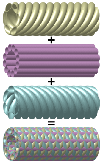
Figure 2: The bottom image is an example of a generation $2$ structure or column, which consists of three intersecting sub-structures that are shown in the top three images. Each sub-structure is composed of hollow cylindrical shells, with one sub-structure having the cylinders aligned parallel to the long axis of the entire column, and in the other two sub-structures the cylinders are wrapped in a helical arrangement (left handed for one sub-structure and right-handed for the other).

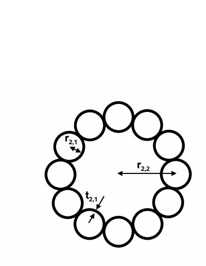
Figure 3: Section through one of the sub-structures in Fig. 2, which has the component hollow cylinders parallel to the axis of the entire generation $2$ structure. The figure shows definitions of various lengths required to specify a generation $2$ structure.

IV The generation $G$ structure

To make the generation $3$ structure, we imagine replacing all the curved but solid shells in a generation $2$ structure (which are of uniform thickness $t_{2,1}$) with composite shells, as described for a flat plate in section II above.

The thinnest (solid) shells comprising this new structure have a thickness of $t_{3,1}$ and compose thin cylinders of radius $r_{3,1}$. These form the substructures of curved shells with effective elastic thickness $t_{3,2}$. These curved shells form cylinders of radius $r_{3,2}$ which compose the substructures of a new composite shell, which is of effective elastic thickness $t_{3,3}$, and from this final doubly-composite shell, a hollow cylinder of length $L$ and radius $r_{3,3}$ is formed, which is the final generation $3$ structure.

By iterating this process, we end up with a generation $G$ structure. In general, $r_{G,m}$ is the radius of each of the (usually composite) cylinders at hierarchical level $m$ of the generation $G$ structure: $r_{G,1}$ is the radius of the smallest (non-composite) cylinders and $r_{G,G}$ that of the multiply composite column itself. Similarly $t_{G,m}$ is the effective elastic thickness of the curved (and usually composite) shells making up the cylinders at hierarchical level $m$ in the generation $G$ structure.

We assume that

$$t_{G,1}\ll r_{G,1}\lesssim t_{G,2}\ll r_{G,2}\lesssim\ldots\lesssim t_{G,G}\ll r_{G,G}\ll L$$ (20)

and by definition we can say the following:

$$t_{G,1}\equiv s_{G,1},$$ (21)

$$Y_{G,1}\equiv Y,$$ (22)

$$\nu_{G,1}\equiv\nu.$$ (23)

The material thickness of the different composite shells are related to one another through Eq. (18) by

$$s_{G,m}=3\pi s_{G,m-1}$$ (24)

and therefore the total (non-dimensionalised) volume of material used is given by

$$v(G)=2\pi Lr_{G,G}s_{G,G}/L^{3}.$$ (25)

The effective elastic properties for $m\in\left\{2,\ldots,G\right\}$ are related to one another in the ghost approximation (which gives an upper bound on $v$) by results analogous to Eqs. (15), (16) and (17) of section II; namely

$$t_{G,m}=\sqrt{6}r_{G,m-1},$$ (26)

$$Y_{G,m}=\frac{\pi}{\sqrt{6}}\left(\frac{t_{G,m-1}}{r_{G,m-1}}\right)Y_{G,m-1},$$ (27)

$$\nu_{G,m}=1/3.$$ (28)

At the largest length scale (i.e. the column itself), the structure is subject to Euler buckling and therefore the largest (non-dimensionalised) force it can support is subject to the constraint

$$f<\frac{1}{YL^{2}}\frac{\pi^{2}I_{G}Y_{G,G}}{L^{2}},$$ (29)

where the relevant second moment of the cross sectional area about the neutral axis is given by

$$I_{G}=\pi t_{G,G}r_{G,G}^{3}.$$ (30)

For the constraints due to localised buckling, we proceed as follows: at the largest length scale, there is one (multiply composite) cylinder aligned with the long axis of the column. This fact is captured by the equation $n_{G,G}=1$.

At the other length scales, we count the number of smaller cylinders in the substructures which are aligned with the long axis of the entire column in the following recursive manner, based on Eq. (19):

$$n_{G,m-1}=\pi\frac{r_{G,m}}{r_{G,m-1}}n_{G,m},$$ (31)

where $m\in\left\{2,\ldots,G\right\}$.

Each of these cylinders at a level $m$ of the structure has a shell with an effective elastic thickness of $t_{G,m}$, effective Young modulus $Y_{G,m}$, effective Poisson ratio $\nu_{G,m}$ and supports a force no more than

$$F_{G,m}\equiv\frac{F}{n_{G,m}},$$ (32)

which we obtain by neglecting the support provided by the other two helically arranged sub-structures at this level (and so on recursively).

As discussed in section II we make the crude approximation that the local buckling condition for a composite shell can be obtained from that for the isolated cylinders composing it. This again uses the ghost approximation, but in this case the approximation no longer provides a strict bound. The result is a sequence of conditions to avoid local buckling at each hierarchical level in the structure, analogous to Eq. (3) and given by

$$F_{G,m}<\frac{2\pi Y_{G,m}t_{G,m}^{2}}{\sqrt{3(1-\nu_{G,m}^{2})}}.$$ (33)

We now proceed to solve the recursion relations of Eqs. (21-24), (26-28) and (31), keeping first of all $t_{G,1}$ and $r_{G,m}$ as parameters for optimisation:

$$s_{G,m}=(3\pi)^{m-1}t_{G,1}$$ (34)

$$t_{G,m}=\left\{\begin{array}[]{cc}t_{G,1}&m=1\\ \sqrt{6}r_{G,m-1}&2\leq m\leq G\end{array}\right.$$ (37)

$$Y_{G,m}=\left\{\begin{array}[]{cc}Y&m=1\\ \frac{\pi^{m-1}}{\sqrt{6}}\left(\frac{t_{G,1}}{r_{G,m-1}}\right)Y&2\leq m\leq G\end{array}\right.$$ (40)

$$\nu_{G,m}=\left\{\begin{array}[]{cc}\nu&m=1\\ 1/3&2\leq m\leq G\end{array}\right.$$ (43)

$$n_{G,m}=\pi^{G-m}\frac{r_{G,G}}{r_{G,m}}.$$ (44)

The condition to be at the limit of Euler buckling (Eq. (29)) therefore becomes

$$f=\frac{\pi^{G+2}}{L^{4}}r_{G,G}^{3}t_{G,1},$$ (45)

the condition to be at the limit of local buckling at the smallest scale of the structure is (from Eqs. (32), (33) and (44))

$$f=\frac{2\pi^{G}}{L^{2}\sqrt{3(1-\nu^{2})}}\frac{r_{G,G}t_{G,1}^{2}}{r_{G,1}},$$ (46)

and to be at the limit of local buckling at the other levels in the structure, gives (from Eqs. (32), (33), (44) and (26)) for $2\leq m\leq G$

$$f=\frac{3\pi^{G}}{L^{2}}\frac{r_{G,m-1}r_{G,G}t_{G,1}}{r_{G,m}}.$$ (47)

Eqs. (25), (34), (45), (46) and (47) can be solved for $G>1$ to give finally

$$v(G)=2^{(1+G)/(2+G)}3^{(2G^{2}-1)/[2(2+G)]}\pi^{(G-2)/(2+G)}$$

$$\times(1-\nu^{2})^{1/[2(2+G)]}f^{1-[1/(G+2)]},$$ (48)

$$\frac{t_{G,1}}{L}=2^{-3/[2(2+G)]}3^{(9-6G)/[4(2+G)]}\pi^{-(2G^{2}-G+2)/[2(2+G)]}$$

$$\times(1-\nu^{2})^{3/[4(2+G)]}f^{(1+2G)/[2(2+G)]},$$ (49)

$$\frac{r_{G,G}}{L}=2^{1/[2(2+G)]}3^{(2G-3)/[4(2+G)]}\pi^{-(3G+2)/[2(2+G)]}$$

$$\times(1-\nu^{2})^{-1/[4(2+G)]}f^{1/[2(2+G)]},$$ (50)

while for $1\leq m<G$

$$\frac{r_{G,m}}{L}=2^{(2G-2m+1)/[2(2+G)]}3^{-(12G-14m+3)/[4(2+G)]}$$

$$\times\pi^{-(2G^{2}-2Gm-G+4m+2)/[2(2+G)]}$$

$$\times(1-\nu^{2})^{-(2G-2m+1)/[4(2+G)]}f^{(1-2m+2G)/[2(2+G)]}.$$ (51)

As a simple practical example, consider a strut of length $L=200{\rm m}$ which is required to support a force of $F=10{\rm kN}$, and which is made from a model material, similar to steel, with $Y=210{\rm GPa}$, $\nu=0.29$ and a density of $8000{\rm kgm}^{-3}$, so that $f=1.2\times 10^{-12}$.

A cable supporting this force under tension would require a mass of $8{\rm kg}$ (assuming a yield stress for the material of $200{\rm MPa}$, and neglecting the mass of couplings at the ends). The masses ($M$) of “steel” required for various structures described in this paper are shown in Table 1.

Table 1: Example calculation for the mass $M$ if a structure required to support $F=10{\rm kN}$ over a distance of $L=200{\rm m}$ when the structure is made from a material similar to steel, with $Y=210{\rm GPa}$, $\nu=0.29$ and density $\rho=8000{\rm kgm}^{-3}$.

$G$	$M$	$t_{G,1}$	$r_{G,1}$	$r_{G,2}$	$r_{G,3}$
0	79 tonnes	-	12.5cm	-	-
1	941kg	0.12mm	81cm	-	-
2	319kg	1.4$\mu$m	1.2mm	2.4m	-
3	261kg	63nm	14$\mu$m	8.2mm	4.6m

Figure 4: Plot of $\log_{10}(v)$ versus $\log_{10}(f)$ for the optimal structures with $G=0,1,2,3,4,5,6$, using Eq. (48) from the text and $\nu=0.29$. The curves are only drawn for the range of $f$ where $r_{G,G}/L\leq 1/20$, $r_{G,m}/r_{G,m+1}\leq 1/20$ and $t_{G,1}/r_{G,1}\leq 1/20$, which we take as an approximation to the condition of Eq. (20) in the text.

Lastly, we note that for a given value of $f$, several generations of structures may be compatible with the conditions of Eq. (20), as illustrated in Fig. 4. In the limit $f\rightarrow 0$, we can calculate the envelope of these curves in order to obtain the global optimally efficient structure within this class, through solving Courant

$$v=v(G)$$ (52)

$$\frac{\partial v(G)}{\partial G}=0,$$ (53)

where $v(G)$ is given by Eq. (48).

In the limit of small $f$, we can expand the exponent of Eq. (52) in powers of $1/G$ to obtain the assymptotic results

$$v\sim\frac{2\pi f}{9}\exp\left[2\sqrt{(\ln 3)(\ln f^{-1})}\right],$$ (54)

$$G\sim\sqrt{\frac{\ln f^{-1}}{\ln 3}}.$$ (55)

V conclusions

We have described compression members consisting of intersecting curved shells in a fractal or hierarchical arrangement which are highly mechanically efficient in the limit of light compressional loading.

Fractal designs for efficient plates under gentle pressure loading have recently been studied in Ref. Farr . In this work, the fractal design arises from two competing tendencies in the structure: Firstly there is a geometrical feature of the plate (narrow, tall spars) which when developed to extremes can lead to very high mechanical efficiency. Secondly, there is a limit to how far this feature may be developed, which is ultimately a vulnerability to buckling. One spar can however be used to provide partial support for another, and this leads to the final hierarchical design.

The parallels with the problem of the present paper should be apparent, and so we suspect that fractal forms may be a general property of optimal elastic structures under gentle and at least partially compressive loading.

At this stage, we are not able to frame a precise mathematical conjecture, and we do not know how other parameters will figure in the analysis. In previous work brittleness Farr was important, and it seems highly probable that in the present work, the amplitude of imperfections in either the geometry or the uniformity of the loading could be crucial to determining the mechanical efficiency Timoshenko ; Timoshenko2 .

We therefore hope that further examples, and perhaps ultimately theorems, will shed light on a problem whose geometrical solutions promise to be useful and even beautiful.

- (1) B. B. Mandelbrot, The Fractal Geometry of Nature (W. H. Freeman & Co., New York, 1983).
- (2) M. Y. Lin, H. M. Lindsay et al., Nature 339(6223), 360 (1989).
- (3) Y. Kantor and I. Webman, Phys. Rev. Lett. 52(21), 1891 (1984).
- (4) M. B. Isichenko, Rev. Mod. Phys., 64(4), 961 (1992).
- (5) G. B. West, J. H. Brown and B. J. Enquist, Science 276(5309), 122 (1997).
- (6) R. Huiskes, Nature 405(6787), 704 (2000).
- (7) D. K. Jacobs, Paleobiology 16(3), 336 (1990).
- (8) R. J. Batt, Lethaia 24(2), 219 (1991).
- (9) R. S. Farr, Phys. Rev. E 76, 046601 (2007).
- (10) L. Euler, Memoires de l’academie des sciences be Berlin 13, 252 (1759). Reprinted in: V. N. Vagliente and H. Krawinkler, J. Eng. Mech.-ASCE 113(2), 186 (1987).
- (11) S. P. Timoshenko and J. M. Gere, Theory of Elastic Stability (McGraw Hill, 1986).
- (12) H. L. Cox, The design of structures of least weight (Oxford, Pergamon Press, 1965).
- (13) J. E. Gordon, Structures (Penguin Books Ltd. 1986).
- (14) W. T. Koiter, On the stability of elastic equilibrium (PhD thesis, Technische Hogeschool Delft, The Netherlands, 1945). English translation issued as: NASA, Tech. Trans., F10, 833 (1967).
- (15) S. P. Timoshenko and S. Woinowsky-Kreiger, Theory of Plates and Shells (McGraw-Hill international, 1989).
- (16) T. von Karman, Collected Works (Butterworth, London 1956).
- (17) A. E. Lobkovsky, Phys. Rev. E 53(4), 3750 (1996).
- (18) R. Courant and D. Hilbert, Methods of Mathematical Physics, Volume 1 (Wiley, 1989).