Imprints of Dark Energy on Cosmic Structure Formation:
II) Non-Universality of the halo mass function

Abstract

The universality of the halo mass function is investigated in the context of dark energy cosmologies. This widely used approximation assumes that the mass function can be expressed as a function of the matter density $\Omega_{m}$ and the root-mean-square linear density fluctuation $\sigma$ only, with no explicit dependence on the properties of dark energy or redshift. In order to test this hypothesis we run a series of 15 high-resolution N-body simulations for different cosmological models. These consist of three $\Lambda$CDM cosmologies best fitting WMAP-1, 3 and 5 years data, which are used for model comparison, and three toy-models characterized by a Ratra-Peebles quintessence potential with different slopes and amounts of dark energy density. These toy models have very different evolutionary histories at the background and linear level, but share the same $\sigma_{8}$ value. For each of these models we measure the mass function from catalogues of halos identified in the simulations using the Friend-of-Friend (FoF) algorithm. We find redshift-dependent deviations from a universal behaviour, well above numerical uncertainties and of non-stochastic origin, which are correlated with the linear growth factor of the investigated cosmologies. Using the spherical collapse as guidance, we show that such deviations are caused by the cosmology dependence of the non-linear collapse and virialization process. For practical applications, we provide a fitting formula of the mass function accurate to 5 percents over the all range of investigated cosmologies. We also derive an empirical relation between the FoF linking parameter and the virial overdensity which can account for most of the deviations from an exact universal behavior. Overall these results suggest that measurements of the halo mass function at $z=0$ can provide additional constraints on dark energy since it carries a fossil record of the past cosmic evolution.

1 Introduction

In this series of articles we have investigated the imprint of dark energy on the non-linear structure formation. In a previous paper (Alimi et al., 2010) we focused on the non-linear matter power spectrum at $z=0$ and showed that dark energy leaves distinctive signatures through a number of effects. On the one hand the clustering of dark energy modifies the shape and amplitude of the linear matter power spectrum, on the other hand the values of the cosmological parameters, such as the matter density $\Omega_{m}$ and the linear root-mean-square (rms) density fluctuations on the $8$ h^-1Mpc scale, $\sigma_{8}$, differ from one model to another such as to satisfy the constraints from Supernova Ia and Cosmic Microwave Background (CMB) observations. Because of this, the shape and amplitude as well as the evolution of the linear power spectrum are affected, with the non-linear phase of collapse mixing and amplifying these model dependent features. This is a direct consequence of the fact that a record of the past history of forming structures is kept throughout the non-linear regime (see e.g. Ma, 2007). Although current measurements of the clustering of matter at small scales are unable to detect such imprints (mainly because of astrophysical systematic uncertainties related to galaxy bias), these effects are present and may become detectable with future weak lensing observations (see e.g. Takada04). Another consequence is that any estimate of the non-linear power spectrum based on parametrized fitting functions written in terms of the cosmological parameters (e.g. $\Omega_{m}$) and instantaneous linear quantities (such as the linear matter power spectrum, $P(k)$, at $z=0$ and the linear growth factor) are of limited precision on the non-linear scales. For instance this is the case of the Smith et al. (2003); Peacock & Dodds (1996) formula. Deviations with respect to these fitting functions depend on the past evolutionary history of a given cosmology, hence it is not surprising that such discrepancies have been found to be manifestly accentuated in the context of dark energy cosmologies (McDonald et al., 2006; Ma, 2007; Francis et al., 2007; Casarini et al., 2009; Jennings et al., 2010; Alimi et al., 2010).

The halo density profile is another observable for which similar effects occur. For example Wechsler et al. (2002) have shown that the concentration parameters depend on the halo assembly history, and it has been shown that such dependencies are strengthened in the case of dark energy models (see for instance Dolag et al., 2004). Paradoxically, as a result of state-of-the-art numerical simulations (Jenkins et al., 2001; Warren et al., 2006), a universal form of the halo mass function entirely specified by $\Omega_{m}$ and linear root-mean-square (rms) density fluctuations $\sigma$ is usually assumed. Furthermore it has been claimed that such a universal form holds for dark energy cosmologies as well (Linder & Jenkins, 2003). If universality is rigorously exact, then in the light of the previous results on the non-linear matter power spectrum and halo profile, it would imply that there must exist an unknown gravitational mechanism capable of erasing the influence of the past evolution of forming structures on the halo mass function. Only in such a case a dependence on cosmology (e.g. the properties of dark energy) and redshift would be absent.

The universality of the mass function at very high-redshift ($z>5$) has been long debated in the literature. As an example deviations from a universal behaviour up to $50\%$ have been found by Reed et al. (2003, 2007). However Lukić et al. (2007) have shown that most of these deviations might be caused by numerical artifacts (finite volume effects or initial conditions set at very low redshift). In fact results inferred from high redshift simulations are very sensitive to numerical errors, consequently several works have focused on the low-redshift mass function. As an example Tinker et al. (2008) have shown deviations from universality up to $30\%$ in the low redshift mass function ($z<3$). Such deviations are thought to be associated with the Spherical Overdensity (SO) halo finder which tends to underestimate the mass function relative to the Friend-of-Friend (FoF) algorithm when considering higher redshifts (Lukić et al., 2009). Since the SO detection is similar to the observational procedure of measuring the mass of galaxy clusters (Tinker et al., 2008), such an effect is more relevant from an observational stand point, but less informative for a better understanding of the non-linear structure formation. To our knowledge, $10\%$ deviations from universality (as a function of redshift) using FoF halo finder have been detected by Lukić et al. (2007); Tinker et al. (2008) at low redshift and very recently confirmed by Crocce et al. (2010). Nonetheless the physical origin of these deviations has yet to be understood, especially in the context of dark energy cosmologies.

Is the halo mass function really universal? To what extent does the universality approximation hold? For which cosmologies and for which redshifts? If there are deviations from an universal behaviour are these of stochastic nature or do they correlate with physical effects? What can we learn from deviations to a universal behaviour and how to model them? These are the questions which we will address in this work.

The paper is organized as follows. In Section 2 we introduce the halo mass function, describe the main features of the cosmological models for which we have run a series of N-body simulations, and discuss the spherical collapse model. In Section 3 we describe the characteristics of the N-body simulations, and the halo finder algorithm, while in Section 4, we discuss various numerical tests which we have performed to identify potential sources of systematics errors. In Section 5, we present the results of the non-universality of the mass function, and discuss the mechanisms responsible for the measured deviations in Section 6. We finally discuss our conclusions in Section 7.

2 Dark energy and structure formation

2.1 The halo mass function

Current analytical predictions of the halo mass function are based on the original work by Press & Schechter (1974). The basic idea is that virialized objects of mass $M$ correspond to regions where the linear density fluctuation field smoothed on the scale $R$ lies above a critical density contrast threshold $\delta_{c}$. Then the halo mass function is simply proportional to the fraction of volume occupied by the collapsed objects with mass greater than $M$. Assuming a Gaussian distribution of density fluctuations, this is given by:

$$F(>M)=\frac{2}{\sqrt{2\pi}\sigma}\int_{\delta_{c}}^{\infty}e^{-\frac{\delta^{2}}{2\sigma^{2}}}d\delta,$$ (1)

where

$$\sigma^{2}(R)=\frac{1}{2\pi^{2}}\int_{0}^{\infty}k^{2}P(k)W^{2}(k,R)dk,$$ (2)

is the variance of the density field smoothed on the scale $R$, with $P(k)$ being the linear matter power spectrum today and $W(k,R)$ is the window function. For a spherical top-hat filter in real space of radius $R$ containing a mass $M\approx 4\pi\bar{\rho}_{0}/3R^{3}$ where $\bar{\rho}_{0}$ is the present matter density, we have $W(k,R)=3\times(sin(kR)/(kR)^{3}-cos(kR)/(kR)^{3})$. The only additional ingredient needed to solve the model is the overdensity threshold $\delta_{c}$, which is assumed to be given by the spherical collapse model prediction of the linearly extrapolated density fluctuation at the time of collapse.

Subsequent studies of the mass function have largely improved this simple modelling (Bond et al., 1991; Lacey & Cole, 1993), and corrections have been included to account for the ellipsoidal collapse (Audit et al., 1997; Sheth & Tormen, 1999; Sheth et al., 2001). Recently a modelling of the halo mass function in the context of the excursion set formalism as well as its extension to the case of non-gaussian initial conditions has been presented in (Maggiore & Riotto, 2009).

A clear understanding of what universality of the mass function implies can be gathered by writing Eq. (1) as

$$F(>M)=\int^{\infty}_{0}S\left(\delta,\frac{\delta}{\sigma}\right)\mathcal{F}\left(\frac{\delta}{\sigma}\right)d\left(\frac{\delta}{\sigma}\right),$$ (3)

where $S(\delta,\delta/\sigma)$ is a selection function in $\delta$-space and $\mathcal{F}$ is the probability distribution of the primordial density fluctuations smoothed on the scale $R$ (for more details about the following discussion see Blanchard et al., 1992). In such a case the halo mass function reads

$$\frac{dn}{dM}=-\frac{\bar{\rho}_{0}}{M}\frac{1}{\sigma^{2}}\frac{d\sigma}{dM}\int^{\infty}_{0}\delta\frac{\partial S}{\partial\delta}\mathcal{F}\left(\frac{\delta}{\sigma}\right)d\delta.$$ (4)

This very general formulation should be a good approximation for slowly evolving primordial power spectra (such as the one used in this paper). A crucial point resulting from Eq. (4) is that all effects associated with the non-linear collapse are encoded in the form of the selection function $S$. Although the precise shape of $S$ is difficult to compute, one may expect as a general trend that $S$ varies from zero to one near the non-linear density threshold $\delta_{S}$. In the end it is this threshold that determines the precise form of the mass function. For instance, by assuming $S$ to be a Heaviside in $\delta_{S}$, one recovers the Press-Schechter halo mass function,

$$\frac{dn}{dM}=-\frac{\bar{\rho}_{0}}{M}\frac{1}{\sigma^{2}}\frac{d\sigma}{dM}\mathcal{F}\left(\frac{\delta_{S}}{\sigma}\right)\delta_{S}.$$ (5)

The dependence on $\delta_{S}$ accounts for the effect of the non-linear gravitational collapse and the virialization process. The former is estimated in terms of the extrapolated linear density at the time of collapse $\delta_{c}^{S}$, and the latter by the virial overdensity at the same time $\Delta_{vir}^{S}$. Since the collapse and virialization processes are specific to each mass, redshift and cosmology, we can expect $\delta_{S}$ to be cosmology and redshift dependent, and consequently, for a given $\sigma$ the mass function as well. This is explicitly manifest in the Press-Schechter (PS) mass function formula, with $\delta_{S}\equiv\delta_{c}$

$$\frac{dn}{dM}=-\frac{\bar{\rho}}{M}\frac{1}{\sigma^{2}}\frac{d\sigma}{dM}f\left(\frac{\delta_{c}}{\sigma}\right)$$ (6)

where the functional form of $f$ is given by:

$$f_{PS}\left(\frac{\delta_{c}}{\sigma}\right)\equiv\mathcal{F}\left(\frac{\delta_{c}}{\sigma}\right)\delta_{c}=\left(\frac{2}{\pi}\right)^{1/2}\frac{\delta_{c}}{\sigma}e^{-\delta_{c}^{2}/(2\sigma^{2})}\cdot$$ (7)

While, in the case of the Sheth-Tormen formula (ST) (Sheth & Tormen, 1999; Sheth et al., 2001), the functional form of $f$ is given by:

$$f_{ST}\left(\frac{\delta_{c}}{\sigma}\right)=A\left(\frac{2a}{\pi}\right)^{1/2}\frac{\delta_{c}}{\sigma}\left[1+\left(\frac{\delta_{c}}{\sigma\sqrt{a}}\right)^{-2p}\right]e^{-\delta_{c}^{2}a/(2\sigma^{2})},$$ (8)

with $A=0.322$, $a=0.707$ and $p=0.3$. Again in these formula $\delta_{c}$ is the spherical collapse prediction of a given cosmology, nevertheless the cosmology dependence encoded in $\delta_{c}$ is often neglected in the literature (see however Percival (2005); Francis et al. (2009a, b); Grossi & Springel (2009)). This is because the spherical collapse model in the SCDM scenario, which has been for long time the reference cosmology to study structure formation, predicts $\delta_{c}=1.686$ and $\Delta_{vir}=178$ constant in redshift. Therefore it has become common to set $\delta_{c}$ to such a value. Alternatively the functional form of $f$ in Eq. (6) has been directly fitted against the mass function measured in numerical simulations as a function of $\sigma$ only (Jenkins et al., 2001; Linder & Jenkins, 2003; Warren et al., 2006). For example, Jenkins et al. (2001) found

$$f(\sigma)=0.315\exp{(-|\ln{\sigma^{-1}}+0.61|^{3.8})},$$ (9)

over the range $-1.2\leq\ln{\sigma^{-1}}\leq 1.05$, with deviations for different cosmologies within $20\%$ level. In such a case Eq. (6) depends on the matter density $\Omega_{m}$ and the rms linear density fluctuation $\sigma$ only, thus manifestly independent of the specificities related to the cosmological and redshift evolution of the non-linear collapse and virialization process. This is what is commonly understood as “universality” of the mass function. Another way of rephrasing this idea is to say that the function $f$ in Eq. (6)

$$f(\sigma)\equiv\int_{0}^{\infty}\delta\frac{\partial S}{\partial\delta}\mathcal{F}(\frac{\delta}{\sigma})d\delta,$$ (10)

is universal if the selection function $S$ is independent of cosmology and redshift. How exact is this statement, and to what extent it remains valid especially in the context of dark energy cosmologies?

Figure 1: Relative variation of $f(\delta_{c}/\sigma)$ for different values of the spherical collapse derived density threshold $\delta_{c}$ as a function of $\ln(\sigma^{-1})$. Top panel shows variation for the Press-Schechter formula, while we plot the variation for the Sheth-Tormen formula in the bottom panel. Curves from top to bottom correspond to regularly spaced values of $\delta_{c}$ in the range $1.638$ to $1.686$ (covering the interval of values inferred from the spherical collapse for the cosmological models considered in this paper).

We can have an estimate of the influence of varying $\delta_{S}$ on $f(\sigma)$ by evaluating the relative error

$$\frac{\Delta f}{f}=\frac{\int^{\infty}_{0}\delta\frac{\partial^{2}S}{\partial\delta^{2}}\mathcal{F}(\frac{\delta}{\sigma})d\delta}{\int^{\infty}_{0}\delta\frac{\partial S}{\partial\delta}\mathcal{F}\left(\frac{\delta}{\sigma}\right)d\delta}\Delta{\delta_{S}},$$ (11)

we may notice that deviations from a universal behaviour are proportional to $\Delta\delta_{S}$. In Fig. 1, we illustrate this for the (extended) Press-Schechter (PS) formula and the Sheth-Tormen (ST) parametrization, where we let $\delta_{S}$ ($=\delta_{c}$) varying in the range 1.638 to 1.686 (corresponding to the typical range of $\delta_{c}$ values covered by the cosmological models studied in this paper). We can see that the effect of varying $\delta_{S}$ is more important on the high mass tail of the mass function (i.e. $\ln{(\sigma^{-1})}>0$). This is because the mass function is exponentially sensitive to the value of $\delta_{S}$. It is for this very reason that we will specifically focus on the high mass tail, nevertheless this does not imply that there are no effects on smaller masses. From Fig. 1 we can also notice that the variations induced on $f(\sigma)$ are similar for the PS and ST prescriptions, thus suggesting that we can study deviations from universality independently of the specific form fo the mass function. To this purpose, we focus on models which exhibit the same rms fluctuations $\sigma$, while being characterized by different background expansion histories and evolutions of the linear perturbations.

2.2 Cosmological toy-models: background and linear evolution

We consider as reference cosmology a $\Lambda$CDM model best fit to WMAP-5 years data (Komatsu et al., 2009) which hereafter we refer to as $\Lambda$CDM-W5. For comparison we also consider two additional $\Lambda$CDM models calibrated to WMAP-1 and 3 years data (Spergel et al., 2003, 2007), which we dub as $\Lambda$CDM-W3 and $\Lambda$CDM-W1 respectively. The model parameter values of these $\Lambda$CDM-WMAP cosmologies are listed in Table 1, the most noticeable difference between these models concerns the $\sigma_{8}$ value, nevertheless their expansion and linear growth histories are almost identical as we will discuss later in this Section. In order to investigate the imprint of dark energy on the halo mass function and test the universality hypothesis, we confront the $\Lambda$CDM-W5 cosmology with a set of “toy-models”. These are flat cosmological models with different background expansion and linear growth of the density perturbations. Following the discussion of the previous paragraph we additionally require the models to have the same distribution of linear density fluctuations at $z=0$, hence the same $\sigma_{8}$ value.

Model	$\Omega_{DE}$	$h$	$\sigma_{8}$	$n_{s}$	$\Omega_{b}$
$\Lambda$CDM-W5	0.74	0.72	0.79	0.963	0.044
$\Lambda$CDM-W3	0.76	0.73	0.74	0.951	0.042
$\Lambda$CDM-W1	0.71	0.72	0.90	0.99	0.047

Table 1: Cosmological parameter values of the WMAP calibrated cosmologies. Our reference model is the $\Lambda$CDM-W5.

We focus on a quintessence model with Ratra-Peebles potential (Ratra & Peebles, 1988):

$$V(\phi)=\frac{\lambda^{4+\alpha}}{m_{Pl}^{\alpha}\phi^{\alpha}},$$ (12)

where $\alpha$ and $\lambda$ are the slope and amplitude of the scalar self-interaction respectively, and $\phi$ is the quintessence field evolving according to the Klein-Gordon equation. For $\alpha=0$ the quintessence cosmology resembles a standard $\Lambda$CDM, provided that the initial field velocity vanishes. We choose the RP model since it corresponds to a dark energy component whose equation of state can vary from $w=-1$ (cosmological constant value) to an evolving function of the redshift ($w(z)\geq-1$) by changing the slope of the potential through the parameter $\alpha\geq 0$. As we are specifically interested in cosmological evolutions which largely differs from that of $\Lambda$CDM, we consider a quintessence model with $\alpha=10$, which we dub as L-RPCDM (the letter L in the acronym means large $\alpha$ value).

We also construct two models with different amount of dark energy density. In particular we consider a $\Lambda$CDM model characterized by a large value of the dark energy density, $\Omega_{DE}=0.9$, which we refer to as L-$\Lambda$CDM (here L meaning large $\Omega_{DE}$ value), and a cold-dark matter dominated cosmology, SCDM^∗, with $\Omega_{DE}=0$ or equivalently $\Omega_{m}=1$ (the $*$ symbol is to remind that the other model parameter values differ from the SCDM usually considered in the literature ). In Table 2 we quote the toy-model parameters, while all the other cosmological parameters ($h,n_{s},\sigma_{8},..$) are set to the $\Lambda$CDM-W5 values. An important point is that given the same initial conditions at some early time (e.g. at recombination) these models predict different matter power spectra at $z=0$. However, we would like to investigate deviations from a universal behaviour of the mass function independently of the present form of the matter power spectrum. Therefore we artificially force these models to have the matter power spectrum at $z=0$ of the $\Lambda$CDM-W5 reference cosmology. From a practical point of view this means that when running the N-body simulations, for each model we generate the initial conditions such that the linearly extrapolated matter power spectrum at $z=0$ (obtained by using the growth factor $D^{+}(z)$ specific to each model) coincides with that of the $\Lambda$CDM-W5. Since $D^{+}(z)$ is model dependent, it implies that the various models will have the same initial power spectrum, but a different initial redshift (see Sect.3 and Sect.4 for technical details about this point). We want to stress that such toy-models are not intended to be compatible with observations, contrary to the “realistic models” considered in the previous paper (Alimi et al., 2010) which were calibrated against CMB and SN Ia data. Again, our aim here is to perform a physical study of the cosmological dependence of the mass function. Nonetheless the conclusions drawn from this study will be extended to more realistic cosmological models as well in a forthcoming paper.

Model	$\Omega_{DE}$	$\alpha$	P(k)
L-RPCDM	0.74	10	$\Lambda$CDM-W5
L-$\Lambda$CDM	0.9	-	$\Lambda$CDM-W5
SCDM∗	0	-	$\Lambda$CDM-W5

Table 2: Toy-models characteristics; the values of the other parameters $h$, $\sigma_{8}$ and $n_{s}$ are set to the $\Lambda$CDM-W5 values quoted in Table 1.

Figure 2: Scale factor dependence of the Hubble rate (left column panels), acceleration parameter (middle column panels) and linear growth factor (right column panels) for the RP models with different values of $\alpha=0,1,..,10$ (upper row panels), for $\Lambda$CDM with different values of $\Omega_{DE}=0,0.1,..,1$ (central row panels) and for the WMAP models (lower row panels). In all panels the solid line corresponds to the $\Lambda$CDM-W5; in the upper panels the L-RPCDM model corresponds to the triple-dot-dashed line, while in the central panels the L-$\Lambda$CDM and SCDM^∗ models correspond to the short-dashed and dot-dashed lines respectively. In the bottom panels $\Lambda$CDM-W1 and $\Lambda$CDM-W3 models corresponds to the dotted and long-dashed lines respectively.

In Fig. 2 we plot the Hubble rate $H(a)$, the acceleration parameter $q(a)$ and the linear growth factor $D^{+}(a)/D_{0}^{+}$ for different cosmologies including our toy-models. The Hubble rate and the growth factor are normalized to that of the $\Lambda$CDM-W5 cosmology. In the upper panels we plot RP models with $\alpha=0,1,..,10$; the L-RPCDM model is shown as triple-dot-dashed line. We may notice that the Hubble rate increasingly deviates at higher redshifts from that of the reference cosmology for larger values of $\alpha$ (curves bottom to top in the upper left panel). Similarly, in such models the evolution of the acceleration parameter shows that the expansion is less decelerated during the matter dominated era and less accelerated during the dark energy dominated era (see upper central panel). Besides the acceleration starts later for larger values of $\alpha$, such that above some values (corresponding to dark energy models with equation of state $w>-1/(3\Omega_{DE})$) the acceleration never takes place. As dark energy dominates earlier (for increasing values of $\alpha$) the deviation of the linear growth rate with respect to the $\Lambda$CDM-W5 case is larger at high redshift, with differences up to a factor $2$ at $a=0.1$ (see curves bottom to top in the upper right panel). In the middle panels of Fig. 2 are shown $\Lambda$CDM models (equivalent to RP models with $\alpha=0$) with different amount of dark energy density. The various curves correspond to $\Omega_{DE}=0,0.1,..,1$ (curves bottom to top). The L-$\Lambda$CDM and SCDM^∗ models are plotted as short-dashed and dot-dashed lines respectively. We can see here a trend which is similar to that of varying $\alpha$ in the RP models. However when increasing $\Omega_{DE}$ the deviations on the Hubble rate are much larger compared to the previous case. Moreover, since the dark energy equation of state here is fixed to the cosmological constant value ($\alpha=0$ or $w=-1$), for decreasing values of $\Omega_{DE}$ the acceleration occurs later, and eventually never takes place for sufficiently low values of $\Omega_{DE}$ (corresponding to matter dominated cosmologies). On the other hand we may notice that the linear growth factor deviates from that of the reference cosmology both at low and high redshifts (middle right panel). Finally in the lower panels are shown the $\Lambda$CDM-WMAP models. As we can see these have very similar behaviours both at the background and linear level. Henceforth our toy-models are characterized by a cosmic evolution which differs from that of standard vanilla $\Lambda$CDM cosmology. Deviations on the Hubble rate are up to $40\%$ for the L-RPCDM model, $50\%$ for the L-$\Lambda$CDM and $95\%$ for SCDM^∗ respectively. Also the redshift dependence of the linear growth factor differs from that of the reference cosmology with larger deviations at higher redshifts, up to a factor $2$ at $a=0.1$ for the L-RPCDM model. In the case of L-$\Lambda$CDM and SCDM^∗ such deviations are present both at high and low redshifts and up to $30\%$ level respectively. If the universality hypothesis holds then such differences should not leave any imprint in the halo mass function.

2.3 Cosmological toy-models: spherical collapse

Figure 3: Evolution of $\delta_{c}$ (left panel) and $\Delta_{vir}$ as a function of the redshift of collapse for the different cosmological models, the line coding is the same as in Fig. 2. Note that $\delta_{c}$ and $Delta_{vir}$ for L-RPCDM does tend towards 1.686 and 178 but at very high redshift.

The collapse of a spherical matter overdensity embedded in an expanding Friedmann-Lemaître-Robertson-Walker (FLRW) background is the simplest model to describe the evolution of a density perturbation throughout the non-linear phase of gravitational collapse. For a given cosmology it allows us to estimate the time of collapse of an initial density perturbation, as well as the value of the overdensity at the time of virialization (i.e. assuming that the perturbation virializes at some time before collapse). Formally, the spherical collapse equation describes the evolution of a matter overdensity $\delta_{m}$ with a top-hat profile in a sphere of radius $R$ as derived from the Raychaudury equation and which reads as:

$$\frac{\ddot{R}}{R}=-\frac{4\pi G}{3}(\rho+3p),$$ (13)

where $\rho$ and $p$ are the total energy density and pressure within the sphere. Here we treat dark energy as a homogeneous component presents only at the background level. This is required for consistency with the fact that our N-body simulations do not explicitly account for the presence of dark energy perturbations, except for the linear regime of the realistic model simulations discussed in (Alimi et al., 2010). Hence the halos detected in the simulations are effectively dark matter overdensities embedded in a FLRW background in the presence of a homogeneous dark energy. Since we aim to interpret the properties of these halos using the spherical collapse model, we solve the model equations in a similar cosmological setup.

In such a case the energy density and pressure in the spherical region are given by $\rho=\rho_{m}^{c}+\bar{\rho}_{DE}$ and $p=w_{DE}\bar{\rho}_{DE}$, where $\rho_{m}^{c}\equiv\bar{\rho}_{m}(1+\delta_{m})$ is the matter density in the sphere of radius $R$, while $\bar{\rho}_{m}$ and $\bar{\rho}_{DE}$ are the background matter and dark energy density respectively, with $w$ being the dark energy equation of state. The background densities evolve according to

$$\dot{\bar{\rho}}_{m}+3\frac{\dot{a}}{a}\bar{\rho}_{m}=0,$$ (14)

and

$$\dot{\bar{\rho}}_{DE}+3(1+w)\frac{\dot{a}}{a}\bar{\rho}_{DE}=0.$$ (15)

For the quintessence models considered here the dark energy density and equation of state depends are given in terms of the scalar field potential and kinetic energy $\bar{\rho}_{DE}=\dot{\phi}^{2}/2+V(\phi)$ and $w=\frac{\dot{\phi}^{2}/2-V(\phi)}{\dot{\phi}^{2}/2+V(\phi)}$, with the scalar field $\phi$ evolving according to the Klein-Gordon equation which we solve numerically. The evolution of the local matter density inside the sphere is given by

$$\dot{{\rho}}_{m}^{c}+3\frac{\dot{R}}{R}{\rho}_{m}^{c}=0.$$ (16)

Integrating Eq. (16) and substituting the definition of $\rho_{m}^{c}$ in terms of the background matter density, we find the relation between $\delta_{m}$ and $R$ at time $t$,

$$1+\delta_{m}=(1+\delta_{m}^{i})\left(\frac{a}{a_{i}}\right)^{3}\left(\frac{R_{i}}{R}\right)^{3},$$ (17)

where $\delta_{m}^{i}$, $a_{i}$ and $R_{i}$ are the matter overdensity, scale factor and radius at the initial time $t_{i}$. Finally using Eq. (17) we can rewrite Eq. (13) in terms of a second order differential equation for the spherical matter overdensity (Nunes & Mota, 2006; Abramo et al., 2007, see also):

$$\ddot{\delta}_{m}+2H\dot{\delta}_{m}=4\pi G\bar{\rho}_{m}\delta_{m}(1+\delta_{m})+\frac{4}{3}\frac{\dot{\delta}^{2}_{m}}{1+\delta_{m}}.$$ (18)

Equation (18) is a non-linear ODE, which at the linear order reduces to the standard equation for spherical linear matter perturbations in the presence of a homogeneous dark energy component (see e.g. Creminelli et al., 2009, in the inhomogeous case). Notice that dark energy affects the matter spherical collapse only because of its influence on the background dynamics through the friction term appearing in Eq. (18).

Past works have solved the spherical collapse using Eq. (13), however we prefer to work with Eq. (18) which we solve numerically as an initial conditions problem rather than a boundary value one as in the case of Eq. (13). This allows us to relax some the assumptions used in the literature, such as estimating the time of collapse $t_{c}$ assuming that $t_{c}=2t_{ta}$, where $t_{ta}$ is the time of turn-around, i.e. when $\dot{R}=0$ after an initial phase of radial expansion. Besides by solving the linearized form of Eq. (18) for the same set of initial conditions that lead to collapse at $t_{c}$ (or equivalently $z_{c}$), we are able to directly infer the value of the linear density contrast at the time of collapse, $\delta_{c}$, without the need of using semi-analytical formula for the linear growth factor. In order to numerically solve Eq. (18), we first rewrite it in terms of the redshift variable $z$ (i.e. $\frac{d}{dt}=\frac{d}{dz}\frac{dz}{dt}$, hereafter ${}^{\prime}=d/dz$) and set initial conditions with the perturbation $\delta_{m}^{i}$ initially starting in the Hubble flow ($\dot{R}_{i}/R_{i}=H_{i}$, i.e. ${\delta_{m}^{i}}^{\prime}=0$). At the beginning the system evolves linearly, but as the quadratic terms in Eq. (18) become non-negligible the collapse enters in the non-linear evolution which ultimately leads to a diverging non-linear matter density contrast, $\delta_{m}\rightarrow\infty$, at the redshift of collapse $z_{c}$ (corresponding to the radius of the spherical region $R\rightarrow 0$). Since our goal is to determine the linear density contrast for a perturbation collapsing at $z_{c}=0$ and more generally at a given $z_{c}$, we have implemented a numerical algorithm which iteratively searches for the initial density perturbation value $\delta_{m}^{i}$ for which $\delta_{m}$ diverges at the input redshift value $z_{c}$. Formally $\delta_{m}(z_{c})=\infty$, but numerically it is not possible to verify such a condition exactly, hence we use an additional algorithm, similar to that developed in London & Flannery (1982), to determine for a given level of accuracy when $\delta_{m}$ reaches the singularity. We fix the accuracy to $\Delta{z_{c}}=10^{-5}$, then the algorithm alts the search for $\delta_{m}^{i}$ as soon as a divergent solution for $\delta_{m}$ is found within $\Delta{z_{c}}$ from the specific $z_{c}$ value of interest. At the same time we calculate on flight the turn-around condition $\delta_{m}^{\prime}=0$ and determine the corresponding redshift $z_{ta}$. Furthermore we numerically solve the linearized form of Eq. (18) using ${\delta_{m}^{i}}^{\prime}=0$ and the $\delta_{m}^{i}$ value previously determined for which collapse occurs at $z_{c}$ to finally infer the value of the linear density contrast at the time of collapse, $\delta_{c}$.

From the spherical collapse dynamics we can also calculate the redshift and the non-linear overdensity value at the time of virialization. In the spherical collapse model, this can be implemented only as an external condition by requiring that at the time of virialization the kinetic energy of the system $T$ and the gravitational potential energy $U$ satisfy the virial condition $T_{vir}=(R_{vir}/2)(\partial{U}/\partial{R})_{vir}$ (see e.g. Peebles, 1993). Then using energy conservation, $T_{vir}+U(z_{vir})={\rm const.}$, one can infer the redshift of virialization by solving the algebraic equation

$$\frac{R}{2}\frac{\partial{U}}{\partial{R}}(z_{vir})+U(z_{vir})=U(z_{ta}),$$ (19)

where we have used the fact that at turn-around the kinetic energy of the system vanishes, $T_{ta}=0$. We refer to Maor & Lahav (2005) for an explicit form of the gravitational potential energy in terms of the matter overdensity and dark energy density for different cosmological set up, including SCDM, $\Lambda$CDM and homogeneous dark energy models. Using the numerical computation previously described we numerically solve Eq. (19) to derive $z_{vir}$ and compute the virial overdensity $\Delta_{vir}\equiv\bar{\rho}_{m}(z_{vir})(1+\delta_{m}^{vir})/\bar{\rho}_{m}(z_{c})$. However we would like to remind the reader that the use of Eq. (19) is rigorously justified only in the SCDM and $\Lambda$CDM models. This is because in the presence of a homogeneous dark energy component for which the background density evolves in time at a rate different from that of the background matter component, energy is not conserved within the spherical overdensity region. Despite several attempts to account for such a loss of energy (see e.g. Maor & Lahav, 2005), we still lack a full relativistic calculation (see discussion in Creminelli et al., 2009). Thus similar to previous analysis the virial overdensity value which we infer for the L-RPCDM model should be considered only as approximative. Given this state-of-art computation we cannot do better.

Model	$\delta_{c}$	$\Delta_{vir}$
$\Lambda$CDM-W5	1.673	368
$\Lambda$CDM-W3	1.672	387
$\Lambda$CDM-W1	1.674	344
L-RPCDM	1.638	436
L-$\Lambda$CDM	1.665	708
SCDM*	1.686	178

Table 3: Values of the linearly extrapolated critical density threshold $\delta_{c}$ and virial overdensity $\Delta_{vir}$ at $z_{c}=0$ predicted by the spherical collapse model. Note that $\Lambda$CDM-WMAP cosmologies have very similar values for the collapse and virialization parameters. The L-RPCDM model differs mainly in the value of $\delta_{c}$, while the effect of varying the dark energy density as described by the SCDM^∗ and L-$\Lambda$CDM models primarily affects the virial overdensity value.

In Table 3 we list the values of $\delta_{c}$ and $\Delta_{vir}$ at $z_{c}=0$ for the different cosmological models. We recover the standard SCDM^∗ values $\delta_{c}=1.686$ and $\Delta_{vir}=178$; the values corresponding to the various $\Lambda$CDM models are consistent with those found in Eke et al. (1996), similarly the values of the L-RPCDM model are compatible with those quoted in Mainini et al. (2003). As expected, the $\Lambda$CDM-WMAP cosmologies have very similar collapse and virialization parameters, this is coherent with the fact that their expansion history and linear growth evolution are very similar as well. In contrast the L-RPCDM model predicts the lowest value, $\delta_{c}=1.638$, which in the framework of the Press-Schechter formalism means that in such a model structures form earlier. The spherical collapse prediction of $\delta_{c}$ for L-$\Lambda$CDM and SCDM^∗ gives $\delta_{c}=1.665$ and $1.686$ respectively, only a few percent lower and higher than those of $\Lambda$CDM-WMAP models. In contrast the former models predict very different values for the virial overdensity ($708$ and $178$ respectively). Since a larger virial overdensity implies a more compact object, we expect that virialized objects tend to be more compact as the amount of dark energy increases.

In Fig. 3 we plot the evolution of $\delta_{c}$ (left panel) and $\Delta_{vir}$ (right panel) as a function of the redshift of collapse. We can see that both the collapse threshold and the virial overdensity is closed to the SCDM values with large $z_{c}$. This is expected since at higher redshift the collapse occurs in a matter dominated universe. The redshift evolution of $\delta_{c}$ in L-RPCDM shows the largest deviation with respect to the trend of the other models, with a much slower convergence toward SCDM. This is because dark energy starts dominating earlier in L-RPCDM than the other cosmological models. In contrast the evolution $\Delta_{vir}(z_{c})$ has the largest deviation for the L-$\Lambda$CDM model, with $\Delta_{vir}$ rapidly decreasing towards high redshifts due to the fact that in such a model the acceleration occurs earlier (see Fig. 2).

The spherical collapse model remains a very simplistic description of the gravitational collapse of structures in the universe. Typically these are not isolated, or spherical, and their velocity dispersion and angular momentum are certainly not negligible. Nevertheless the model captures some features of the non-linear phase of collapse (see for instance Valageas (2009) for analytical results in the rare events limit). It can therefore guide us toward a better understanding of the formation and evolution of dark matter halos as detected in N-body simulations.

3 N-Body simulations

3.1 Simulation sets

The numerical set up is the same as the one presented in Alimi et al. (2010) and we refer the interested reader to the previous article for a detailed description of the numerical codes used in this series of papers. The N-body simulations are performed using the RAMSES-AMR (Adaptative Mesh Refinement) code (Teyssier, 2002; Rasera & Teyssier, 2006) based on a multigrid Poisson solver. The matter power spectra are computed using the CAMB code (Lewis et al., 2000), then Gaussian initial conditions using the Zel’dovich approximation are generated with MPGRAFIC (Prunet et al. (2008)). For the toy-models we use the LCDM-W5 power spectrum (see previous sections). For each model the various cosmological variables ($a(t),H(t)$, etc…) are pre-computed with an independent code and stored into tables, these are subsequently interpolated to input the various time dependent quantities into appropriately modified version of MPGRAFIC and RAMSES. We have used the same phase for the initial conditions of the various simulations, more specifically the white noise from the Horizon Project. We have performed a total of 15 simulations at the “Centre de Calcul Recherche et Technologie” (CCRT). Our longest simulation run for 350 hours of elapsed time on 64 cores. In Table 4 we list the characteristics of the 15 cosmological simulations covering 6 cosmological models at various scales.

Model	162 h-1Mpc	648 h-1Mpc	1296 h-1Mpc
$\Lambda$CDM-W5
$z_{i}$	$93$	$56$	$41$
$m_{p}$ (h-1M⊙)	$2.28\times 10^{9}$	$1.46\times 10^{11}$	$1.17\times 10^{12}$
$\Delta$x (h-1kpc)	$2.47$	$19.78$	$39.55$
$\ell_{\textrm{max}}$	$7$	$6$	$6$
L-RPCDM
$z_{i}$	-	$136$	$97$
$m_{p}$ (h-1M⊙)	-	$1.46\times 10^{11}$	$1.17\times 10^{12}$
$\Delta$x (h-1kpc)	-	$9.89$	$39.55$
$\ell_{\textrm{max}}$	-	$7$	$6$
L-$\Lambda$CDM
$z_{i}$	-	$71$	$52$
$m_{p}$ (h-1M⊙)	-	$5.61\times 10^{10}$	$4.50\times 10^{11}$
$\Delta$x (h-1kpc)	-	$9.89$	$39.55$
$\ell_{\textrm{max}}$	-	$7$	$6$
SCDM*
$z_{i}$	-	$42$	$30$
$m_{p}$ (h-1M⊙)	-	$5.61\times 10^{11}$	$4.50\times 10^{12}$
$\Delta$x (h-1kpc)	-	$19.78$	$79.10$
$\ell_{\textrm{max}}$	-	$6$	$5$
$\Lambda$CDM-W3
$z_{i}$	84	$52$	$38$
$m_{p}$ (h-1M⊙)	$2.11\times 10^{9}$	$1.35\times 10^{11}$	$1.08\times 10^{12}$
$\Delta$x (h-1kpc)	2.47	$79.10$	$158.20$
$\ell_{\textrm{max}}$	7	$4$	$4$
$\Lambda$CDM-W1
$z_{i}$	110	$65$	$47$
$m_{p}$ (h-1M⊙)	$2.55\times 10^{9}$	$1.63\times 10^{11}$	$1.31\times 10^{12}$
$\Delta$x (h-1kpc)	2.47	$19.78$	$39.55$
$\ell_{\textrm{max}}$	7	$6$	$6$

Table 4: Parameters of the 15 N-body simulations for the various cosmological models: $z_{i}$ is the initial redshift, $m_{p}$ is the mass of the particle, $\Delta$x the comoving resolution and $\ell_{\textrm{max}}$ is the maximum refinement level. Each simulation has $512^{3}$ particles, with a $512^{3}$ grid on the coarse level and evolved down to $z=0$. All the simulations share the same realization of the initial conditions (namely the Horizon Project white noise), and start at the same level of rms density fluctuation ($\simeq 0.05$) at the scale of the resolution of the coarse grid. Our refinement strategy consist in refining when the number of particles in one cell is greater than 8.

Since we expect deviations from universality to manifest in the high-mass tail of the mass function, our box lengths of interest are $648~{}{\rm h^{-1}Mpc}$ and $1296~{}{\rm h^{-1}Mpc}$. In the case of the WMAP $\Lambda$CDM cosmologies we have also performed three simulations with a box length of $162{\rm h^{-1}Mpc}$ for comparison with the mass functions at intermediate mass ranges which have been estimated in previous studies.

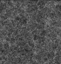
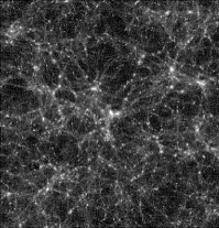
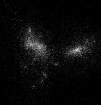
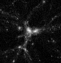
Figure 4: 2-dimensional projection of the dark matter density at z=0 from the $\Lambda$CDM-W5 simulation in the 648 h^-1Mpc box. The four images represent a zooming sequence (clockwise from top to bottom) of a factor four for each image from the full box size (upper left) to a 10 h^-1Mpc scale (bottom left).

In Fig. 4, we illustrate the dynamics of the RAMSES AMR code with a zooming sequence of images of the dark matter particle distribution in the $\Lambda$CDM-W5 at $z=0$ from cosmological to galaxy group scale (clockwise from top to bottom $648~{}{\rm h^{-1}Mpc}$, $162{\rm h^{-1}Mpc}$, $40{\rm h^{-1}Mpc}$ and $10{\rm h^{-1}Mpc}$). Because of the large simulated volume and the high spatial and mass resolutions, these simulations provide a robust statistics of well resolved halos.

3.2 Halo finder and mass function

The halos in the simulation boxes are identified using the Friend-of-Friend halo finder (FoF) (Davis et al., 1985). This algorithm detects halos as group of particles characterized by an intra-particle distance smaller than a given linking length parameter $b$. The algorithm runs over a list of particle coordinates in the box, firstly it regroups all those which are within distance $b$ of an initial particle. Then it moves to the next particle of the group and reiterates the same selection until no new neighbours are found. At this point the algorithm moves onto the next untagged particle repeating the above procedure to detect a new group (halo).

Halos can also be detected using the Spherical Overdensity algorithm (SO, Lacey & Cole, 1994), which provides halo mass estimations similar to that performed observationally, moreover density profiles are directly given by the algorithm. However the halo detection is restricted to spherical geometry, halos can overlap, and the last particles of the list could merge into some unphysical halos. In contrast under the FoF algorithm all particles belong to halos as in the case of the halo model, and it is applicable to non-spherical particle groups as well, though it has tendency to overlink bridged-halos. Therefore FoF and SO are complementary algorithms. Here we use FoF since by relaxing the assumption on spherical symmetry this allows for a better physical study of the collapsed structures in the simulations (as we shall see hereafter).

As can be seen in Fig. 4, halos are much more complicated than spherical isolated objects with a clearly defined radius. Halos in numerical simulations are non-spherical, interacting with their environment, contain lots of subhalos and, moreover the density can vary rapidly. This makes the definition of their boundary somewhat arbitrary. The SO halo definition is based on the enclosed overdensity $\Delta$ in a given spherical region. This implies that it is rather straightforward to run a SO halo finder with threshold given by $\Delta_{vir}$ from the spherical collapse. Similarly, it is possible to run a FoF halo finder with a linking length parameter $b=b_{vir}$, where $b_{vir}$ corresponds to the value of a spherical overdensity $\Delta_{vir}$, provided that a relation between the two is assumed. A practical conversion formula is given by $\Delta/178\approx(0.2/b)^{3}$ (Cole & Lacey (1996)), nevertheless such a conversion is very approximative. A thorough comparison between the FoF and SO algorithms and the accuracy of conversions has been performed in Lukić et al. (2009) (see also Audit et al., 1998). Furthermore since $b_{vir}$ depends on an approximate treatment of the non-linear collapse, its use as a linking length parameter, introduces built-in assumptions on the mass function obtained with FoF($b_{vir}$), which may hide the non-linear contributions associated with the halo formation and virialization process. For these reasons we start by considering the FoF halo finder with a constant $b$, which we set to $b=0.2$. As we will show, our conclusion about universality will be independent of the exact value of $b$, remaining valid in the range $0.1$ to $0.3$ (corresponding to $\Delta_{vir}$ varying roughly from $1424$ to $53$).

One last point concerns the numerical definition of the halo mass function, which reads as

$$\frac{dn(M)}{d\textrm{log}(M)}=\frac{1}{L^{3}}\frac{N}{\Delta\textrm{log}(M)},$$ (20)

where N is the number of halos in a logarithmic mass bin between $\textrm{log}(M)-\Delta\textrm{log}(M)/2$ and $\textrm{log}(M)+\Delta\textrm{log}(M)/2$, with $\Delta\textrm{log}(M)$ the bin width and $L$ the comoving box length. Our default choice of the bin width is very conservative, $\Delta M/M\simeq 0.2$. Moreover when measuring the mass function we focus on mass ranges which corresponds to halos containing at least $350$ particles and Poisson shot noise below the $10\%$ level. As we will discuss in the next Section, such conservative assumptions are necessary to limit the effect of mass resolution, bin size and Poisson noise, which can be important source of systematic errors in the high-mass tail.

4 Numerical Consistency Checks

In this Section we present a detailed study of various source of numerical systematic effects. As result of this analysis we are able to control numerical errors within few percent level, thus validating our final results at the same percentage level.

4.1 Initial conditions

We have performed a series of tests on the initial conditions generated with MPGRAFIC. Firstly, we have checked that the power spectrum of the initial particle distribution is consistent within a few thousandth with the input spectrum from CAMB near the Nyquist frequency (at this high frequencies the Poisson noise is minimal). In addition, we have compared the MPGRAFIC power spectrum with that extracted from the GRAFIC code for the same white noise. After turning off the Hanning filter subroutine in GRAFIC we have found good agreement even at low $k$ (Bertschinger, 1995, 2001). The Hanning filter suppress the high $k$ modes, hence potentially causing unphysical numerical artifacts on the generated particle distribution even in the linear regime. Therefore previous studies that have inadvertently used the Hanning filter may have underestimated the mass function, which is known to be sensitive to the gravitational dynamics on all scales. In our case, the use of the Hanning filter, led to a roughly $10\%$ suppression of the mass function over the full range of masses tested in our simulations ($10^{14}-10^{15}{\rm h^{-1}M_{\odot}}$). Therefore, we preferred not to use this filter.

A further test concerns the choice of the initial redshift of the simulations. This can be responsible for spurious effects due to transients from initial conditions when using the Zel’dovich approximation (Reed et al., 2003, 2007; Crocce et al., 2006; Lukić et al., 2007). Several works (Crocce et al. (2006), Tinker et al. (2008) and Crocce et al. (2010)) suspect that a very low initial redshift combined with the Zel’dovich approximation might be responsible for the discrepancies between their estimated mass functions and those inferred by Jenkins et al. (2001) and Warren et al. (2006). To be as conservative as possible we have chosen higher initial redshifts $z_{i}$ compared to previous studies (Sheth et al., 2001; Jenkins et al., 2001; Warren et al., 2006). This is realized by imposing that the standard deviation of the density fluctuations smoothed at the scale of the coarse grid $\Delta^{coarse}_{x}$ is $\sigma(\Delta_{x}^{coarse})=0.05$. With this choice our $z_{i}$ for the different cosmologies and simulations boxes vary in the range $30-110$, which are much higher then for instance the initial redshifts considered in Warren et al. (2006) which range from $24$ to $34$ depending on the box lengths, and for which Crocce et al. (2006) have estimated the suppression of the high-mass tail of the mass function to be of order $10-15\%$.

4.2 N-body code

We have run a series of tests to check the accuracy of the RAMSES code as well as the modifications that have been implemented to account for the quintessence scenario. Firstly, we have verified that for the various models the ratio of the measured power spectrum to the linear prediction from CAMB is constant at the percent level on the large linear scales (k$\simeq$0.01-0.1 h/Mpc) of the simulations at all redshifts (see Alimi et al., 2010). Furthermore, we have checked that by reducing the integration time steps the results remain unchanged, thus validating our implementation of quintessence models in RAMSES. Secondly, we have compared the mass function from the RAMSES simulation of the $\Lambda$CDM-W3 cosmology with box length $648~{}{\rm h^{-1}Mpc}$ and $256^{3}$ particles against a simulation with identical characteristics and same seed for the initial conditions obtained using the GADGET code (Springel et al., 2001; Springel, 2005). We find that the two mass functions are in very good agreement (few percent level) over the range of masses corresponding to halos with more than $350$ particles and less than $10\%$ Poisson noise. Using the Warren et al. (2006) correction does not improve noticeably the inferred mass function below 350 particles. In principle the halo mass correction by Warren et al. (2006) depend on code and/or cosmology. Another point concerns the results of Heitmann et al. (2005, 2008), the authors have computed the mass function with various codes using the same set of initial conditions. They found a scatter of order 10% in the high mass range, the HOT code used in Warren et al. (2006) seems to give lower mass functions than other codes such as GADGET by a factor of about ten percent at $\simeq 10^{15}$ h^-1M_⊙.

Figure 5: Left: residual between the measured mass function and our fitting formula for two $\Lambda$CDM-W5 simulations with box lengths 162 h^-1Mpc and 648 h^-1Mpc at z=0. The number of particles is 512³, the minimal number of particles per halo is 350 and the Poisson noise is less than $10$% (vertical lines). This illustrates the coherence between the simulations. Right: As in the previous figure for two simulations with different realisations of the initial conditions. The box length is 1296 h^-1Mpc and the number of particles 512³.

4.3 Particles, box length, mass and force resolution

Another set of tests concerns the sensitivity of the results to various simulation characteristics. First we have checked the stability of the results when varying the number of particles from $256^{3}$ up to $1024^{3}$, while keeping the same phase of the initial conditions. Assuming 350 particles as a minimum for the halo mass, we find that the mass functions are consistent to better than $5\%$ at all masses. Secondly, we have evaluated the influence of varying the maximum level of refinement in RAMSES from $6$ to $4$. This parameter changes the spatial resolution of the simulations, however we found no effect on the mass functions. Besides in our simulations the refinement level evolves freely, and never reaches the maximum allowed level.

Another important consistency check concerns the coherence of the mass functions as measured from simulations with different box lengths. Discrepancies may indicate effects due to either mass resolution or finite volume. With our conservative choice of a minimum of $350$ particles per halo and $10\%$ level of Poisson noise, the coherence in the mass range of interest is better than $5\%$, as it can be seen in the left panel of Fig. 5, where we plot the difference between the mass function measured in $\Lambda$CDM-W5 simulations at $z=0$ with $512^{3}$ particles and box lengths of $648~{}{\rm h^{-1}Mpc}$ and $1296~{}{\rm h^{-1}Mpc}$ respectively, and the Sheth-Tormen parametrization, Eq. (8), calibrated over the whole set of $\Lambda$CDM-W5 simulations. The vertical dotted lines identify the mass intervals where the Poisson noise is below $10\%$ and halos have at least $350$ particles (the right interval corresponding to $1296~{}{\rm h^{-1}Mpc}$ simulation box and the left one to $648~{}{\rm h^{-1}Mpc}$). We can see that the scatter of the points around the zero residual is well within the $5\%$ level. We did not investigate finite volume effects, or cosmic variance specifically. In fact in our largest box ($1296~{}{\rm h^{-1}Mpc}$), the cosmic variance error on the largest halo masses is likely to be dominated by Poisson shot noise as shown in (Hu & Kravtsov, 2003; Crocce et al., 2010), hence it should be within the $10\%$ level set by our requirement for the Poisson noise. We have also checked the effect of changing the phase of the initial conditions. In the right panel of Fig. 5 we plot the residuals of the measured mass function in $\Lambda$CDM-W5 simulations at $z=0$ with box lengths of $1296~{}{\rm h^{-1}Mpc}$ and $512^{3}$ particles with two different phases, with respect to the $\Lambda$CDM-W5 best fitting formula. In the mass range of interests the differences between the residuals are well within the Poisson errorbars.

Figure 6: Effect on the mass function of varying the bin width and binning strategy. The plots show the residuals between the measured mass functions and our fitting formula Eq. (22) as a function of $\ln(\sigma^{-1})$ for two $\Lambda$CDM-W5 simulations with box lengths 648 h^-1Mpc and 1296 h^-1Mpc at z=0. The minimal number of particles per halo is 350 and the Poisson noise is less than $10$%. Left: bins width $\Delta M/M=0.1$. Middle: $0.25$. Right: $1$. Top raw: “average-mass” bins. Bottom raw: “Centered-mass” bins. Using too large bins decrease the mass function, especially for the “average-mass” bins. To be as conservative as possible we use “centered-mass” bins of width $\Delta M/M\simeq 0.2$.

4.4 FoF code & Mass Binning

We have compared the results from our halo finder code to those obtained using “Halomaker” FoF (Tweed et al., 2009) and found no difference in the measured mass function. We have also performed a study of the influence of varying the bin-width and the binning strategy on the mass function. These tests are particularly important, since some authors (see e.g. Jenkins et al., 2001) have used analytical corrections to remove effects caused by large mass-bins and smoothing functions.

In Fig. 6 we plot the residual mass function of $\Lambda$CDM-W5 simulations at $z=0$ with $512^{3}$ particles and box lengths of $648~{}{\rm h^{-1}Mpc}$ and $1296~{}{\rm h^{-1}Mpc}$ respectively with respect to the Sheth-Tormen best fitting formula, for different bin-widths: $\Delta{M}/M=0.1$ (left panels), $\Delta{M}/M=0.25$ (central panels) and $\Delta{M}/M=1$ (right panels). In the top panels we plot the case with averaged-mass bins, i.e. the mass of each point is the average mass of the halos in the bin, while in the bottom panels we plot the case with centered-mass bins, i.e. the mass of each point is the central value of the logarithmic mass bin. We can see that for both binning strategies increasing the bin-width reduces the Poisson noise and smooths the curves. However increasing the bin size is particularly delicate in the high mass tail especially for the averaged-mass binning. In fact we can see that a larger binning ($\Delta{M}/M=1$) tends to lower the mass function intrinsic scatter. This is because as the bin-size increases, each bin has a larger number of halos thus leading to smaller Poisson errors on the other hand in the high-mass tail the mass function drops steeply and the use of averaged-mass bins tends to lower its value. As noticeable from Fig. 6, such an effect is much weaker in the case of centered-mass bins which we adopt hereafter, and for the study of the universality of the mass function we consider centered-mass bins with width $\Delta{M}/M=0.2$, a compromise between the Poisson noise and the number of bins. It is worth noticing that Jenkins et al. (2001) use large bins and a gaussian smoothing (of rms 0.08 in $\ln{(M)}$ corresponding to a width of 0.37 in our units) which is supposed to strongly raise the curve. An analytical correcting factor is then applied to recover a proper estimate of the mass function. We find this procedure to be quite uncertain. Again as seen in Fig 6 using large bins tends to lower the mass function unlike expectations, and such an analytical correction might cause an underestimate in the high mass end at the $10\%$ level. In such a case, it is safer to use smaller bins such that deviations remain within $5\%$ (as in our case) and not rely on analytical corrections. In the light of these various tests, our precision on the absolute FoF mass function is expected to be of order $5-10\%$. However, we want to stress that the precision on the relative mass function is even higher (typically less than $5\%$) since for all our simulations we use the same phase for the initial conditions, and thus systematic errors cancel out. The Poisson error bars are consequently not relevant for quantifying the error on the relative mass functions, since the scatter of the mass functions in two different cosmologies is strongly correlated. Moreover from the above analysis we can see that intrinsic fluctuations of the measured mass functions for a given cosmology are much smaller than the Poisson error bars.

5 Results

5.1 WMAP-$\Lambda$CDM cosmologies and universality at $z=0$

In Fig. 7 we plot the mass function of the $\Lambda$CDM-WMAP cosmologies at $z=0$ and $1$ measured in $162{\rm h^{-1}Mpc}$, $648{\rm h^{-1}Mpc}$ and $1296~{}{\rm h^{-1}Mpc}$ simulation boxes respectively. Notice the large mass range covered by the simulations, which spans from Milk-Way to cluster size halos ($10^{12}-10^{15}{\rm h^{-1}M_{\odot}}$). In order to test the universality of the mass function it is preferable to work with the function

$$f(\sigma)=\frac{M}{\bar{\rho}_{0}}\frac{dn}{d\textrm{ln}(\sigma^{-1})},$$ (21)

where $dn/d\textrm{ln}(\sigma^{-1})$ is the comoving number of halos per unit of natural logarithm of $\sigma^{-1}$. As mentioned in Section 2.1, if the mass function is universal the selection function accounting for the non-linear collapse in the definition of $f$ is independent of cosmology (i.e. independent of the density threshold). In such a case the function $f$ for different cosmological simulations should be identical to numerical precision.

Figure 7: Mass functions $dn(M)/d\textrm{log}(M)$ for the $\Lambda$CDM-WMAP cosmologies at z=0 (upper curves), and z=1 (lower curves) from $162$ h^-1M_⊙, $648$ h^-1M_⊙ and $1296$ h^-1M_⊙ box lengths simulations. Halos are detected with FoF($b=0.2$). The dotted line is our best fit $\Lambda$CDM-W5 Eq. (22). Crosses correspond to $\Lambda$CDM-W1, stars for $\Lambda$CDM-W3 and triangles to $\Lambda$CDM-W5. The mass functions cover a range from Milky-Way size halos to cluster of galaxies.

In Fig. 8 we plot the function $f$ for the three $\Lambda$CDM-WMAP models at $z=0$ in the range $-0.8<\ln{(\sigma^{-1}})<0.7$. We can see that the data points nicely overlap to numerical precision, this is quite remarkable given the fact that these models have different initial conditions with very different $\sigma_{8}$ values. This implies that changing the initial conditions does not break the universality of the mass function in the $\Lambda$CDM cosmologies, which is in agreement with the results of Jenkins et al. (2001); Warren et al. (2006). Nonetheless we find that the functional form of $f$ differs from standard fitting formula inferred in previous analysis (Sheth et al., 2001; Jenkins et al., 2001; Warren et al., 2006). As an example in Fig. 8 we plot against the simulation data-points the fitting formula Eq. (9) given in (Jenkins et al., 2001). Large deviations with respect to this fit occurs in the high-mass end, instead we find a better fit by using the functional form of the ST formula, with different parameter values calibrated on the $\Lambda$CDM-W5 model simulations. In particular by fixing $\delta_{c}$ to the spherical collapse model prediction of the $\Lambda$CDM-W5 cosmology, $\tilde{\delta}_{c}=1.673$, our best fitting function (using b=0.2) reads as:

$$f(\sigma)=\tilde{A}\left(\frac{2\tilde{a}}{\pi}\right)^{1/2}\frac{\tilde{\delta}_{c}}{\sigma}\left[1+\left(\frac{\tilde{\delta}_{c}}{\sigma\sqrt{\tilde{a}}}\right)^{-2\tilde{p}}\right]e^{-\tilde{\delta}_{c}^{2}\tilde{a}/(2\sigma^{2})},$$ (22)

with $\tilde{A}=0.348$, $\tilde{a}=0.695$ and $\tilde{p}=0.1$.

Figure 8: Mass functions for the $\Lambda$CDM-WMAP cosmologies at z=0, in the $f-\ln(\sigma^{-1})$ plane (as defined in the text) from the $162$ h^-1M_⊙, $648$ h^-1M_⊙ and $1296$ h^-1M_⊙ box length simulations. Halos are detected with FoF($b=0.2$). The continuous line is the $\Lambda$CDM-W5 fit described in this section (Eq. 22) and the dotted line is the Jenkins et al. (2001) fit. The conventions are the same than in Fig. 7. Deviations from universality are below numerical precision.

We plot in Fig. 9 the residual of the measured function $f$ against Eq. (22), we can see that the $\Lambda$CDM-WMAP cosmologies have a universal mass function to $5-10\%$ accuracy level. For comparison we also plot the original ST formula Eq. (8) with $\delta_{c}=1.686$ (dashed line), and the Jenkins et al. one Eq. (9) (dotted line). The former badly reproduce the measured mass functions at ${\rm ln(\sigma^{-1})>-0.5}$, while the latter provide a good description only in the lower mass range (${\rm ln(\sigma^{-1})<0.4}$). In contrast at higher masses there are deviations $>20\%$, thus confirming previous results by Tinker et al. (2008); Crocce et al. (2010).

Figure 9: The residual between the fitting formula Eq. (22) and the measured FoF($b=0.2$) mass functions at z=0 for the “WMAP $\Lambda$CDM cosmologies”. The conventions are the same than in Fig. 7. Halos come from $162$ h^-1M_⊙, $648$ h^-1M_⊙ and $1296$ h^-1M_⊙ box lengths simulations. For reference the Jenkins et al. (2001) (dotted line) and the Sheth & Tormen (1999); Sheth et al. (2001) (here in dashed line) fitting formula are also plotted. We recover the universality up to numerical precision ($5-10\%$).

The fact that in $\Lambda$CDM-WMAP cosmologies the mass function at $z=0$ shows a universal behaviour is not surprising, since from the considerations of Section 2.1 these models despite having different $\sigma_{8}$ values and small differences in the other parameters, they have nearly identical expansion histories, linear growth evolution and spherical collapse model parameters. The spherical collapse model is only approximative we may expect small deviations from universality to be present also in these models, however it is likely that such deviations are within the numerical errors of our simulations.

The universality of the mass function for cosmologies characterized by the same expansion history but different $\sigma_{8}$ values (and slightly different values of the other cosmological parameters) implies that the position of the mass function in the plane $f-\rm{ln}(\sigma^{-1})$ is independent of $\sigma_{8}$ (within the accuracy of our simulations). This is an important point to keep in mind, as we will show in the next Section this will allow us to isolate cosmological dependent effects on the halo mass function, which are related to the record of the past expansion history, and also extend our conclusions on the limits of universality to models with different $\sigma_{8}$ values.

5.2 Dark energy models and the limit of universality

We now focus on the toy-model simulations. In Fig. 10 we show the projected density maps from the $648~{}{\rm h^{-1}Mpc}$ simulation box at $z=0$ zoomed on $40{\rm h^{-1}Mpc}$ (left panels) and $10{\rm h^{-1}Mpc}$ (right panels) scales respectively. Since the simulations have the same initial phase, in order to facilitate a visual comparison between different models we plot their density distribution in the same image with a different color coding for each model. In the top panels are shown the density maps for the $\Lambda$CDM-W5 (red) and L-RPCDM (green), while in the lower panel in addition to the $\Lambda$CDM-W5, we also show the L-$\Lambda$CDM (green) and SCDM^∗ (blue). The differences in the top panels are indicative of the effects related to having a time evolving dark energy with $w(z)\geq-1$, while those in the bottom panels are associated to varying the amount of dark energy density. We can see that in both cases there are no apparent differences in the particle distribution on the $40{\rm h^{-1}Mpc}$ scale. In contrast differences are clearly manifest on the $10{\rm h^{-1}Mpc}$ scale, where the halo concentration seems to differ from one model to another, and the outer parts of halos show different morphologies as well.

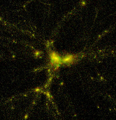
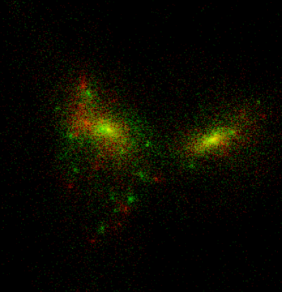
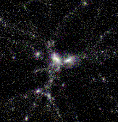
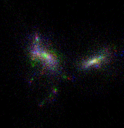
Figure 10: Projected overdensity maps for the $\Lambda$CDM-W5 and L-RPCDM models (top) and $\Lambda$CDM-W5, L-$\Lambda$CDM and SCDM^∗ (bottom) on scale $40$ h${}^{-1}Mpc$ (left) and $10$ h${}^{-1}Mpc$ (right) respectively at z=0. The views are centered onto two halos and extracted from simulations of box length $648$ h^-1Mpc with the same realisation of the initial conditions and the same $\sigma_{8}$. Each cosmology is represented with different color coding (but with the same intensity level). Top panels: $\Lambda$CDM (red) and L-RPCDM (green). Here the distinct green or red regions at small scales are non-linear imprints related to the different equation of state evolution between the two models. Bottom panels: $\Lambda$CDM (red), L-$\Lambda$CDM (green) and SCDM* (blue). Here the distinct colored regions on small scales are non-linear signature due to the different amount of dark energy of the models.

In particular, we may notice that in the L-RPCDM case, since $\Omega_{m}$ and $P(k)$ are the same of the reference cosmology, differences in the dark matter distribution are unique signature of the non-linear process of structure formation. In such a case, it is hard to believe that the mass function should remain unaffected, that is to say universal in dark energy cosmologies.

Figure 11: The residuals between the measured mass functions of L-RPCDM (diamonds) and the measured mass functions for $\Lambda$CDM-W5 (triangles) cosmology at z=0. Deviations from universality are clearly above numerical errors ($<5\%$) and correlated with linear growth history. Here the amplitude of the residuals is a signature of the different dark energy equation of state evolution in the L-RPCDM model.

Figure 12: The residual between the measured mass functions of L-$\Lambda$CDM (crosses), SCDM^∗ (squares) and that of $\Lambda$CDM-W5 (triangles) cosmology at z=0. Deviations from universality are clearly above numerical errors ($<5\%$) and correlated with linear growth history of the models. Here the amplitude of the deviation is related to the different amount of dark energy of the models.

For a more quantitative comparison, we plot in Fig. 11 the residual of the function $f(\sigma)$ measured in L-RPCDM with respect to that of the $\Lambda$CDM-W5. As previously mentioned we only plot the mass range in which halos contain at least 350 particles and where the Poisson noise is within $10\%$, thus allowing us to control numerical errors to better than about $5\%$. From this plot we can clearly see deviations from universality at the $10\%$ level, hence well above numerical errors. Similarly in Fig. 12 we plot the case of L-$\Lambda$CDM and SCDM^∗. The former lies about $5\%$ above the $\Lambda$CDM-W5 model, while the latter is roughly $10\%$ below, again these are evidence of departure from universality. However such deviations are not random, they are correlated with the linear growth history of the corresponding model. In fact comparing the evolution of the growth factor of each model (see Fig. 2) with the corresponding amplitude of the mass function residual, we may notice that the greater the deviation in the growth rate history and the larger is the deviation from universality at z=0. This is not the case for the $\Lambda$CDM-WMAP cosmologies which share nearly the same linear growth rate history and therefore their mass functions are universal to numerical precision. The physical origin of such deviations is quite intuitive. The cosmic structure formation is more efficient in the past when the linear growth rate is greater. This is indeed the case for our toy-models. Even though by construction they share the same amount of clustering at the linear level at $z=0$, lots of dense halos were formed earlier and survive at lower redshift since they are decoupled from the cosmic expansion on the larger scales. The same effects are responsible for the imprints which have been shown to affect the non-linear matter power spectrum Ma (2007); Alimi et al. (2010) and halo concentration Dolag et al. (2004); Wechsler et al. (2002). To our knowledge, this is the first time that physical effects leading to a non-universal behaviour of the mass function have been unambiguously shown.

6 Non-universality of the mass function and the non-linear collapse

In this section we will focus on the non-linear processes which are responsible for the departure from a universal behaviour of the mass function. As discussed in Section 2.1, deviations from universality occur if and only if the non-linear collapse of dark matter is cosmology and redshift dependent (or in other words if the relation between the linear and non-linear growth of structures is cosmology and redshift dependent Francis et al. (2009b)). In the Press-Schechter framework this is parametrized by the dependence of the mass function on the threshold density $\delta_{S}$. This suggests that we may gain a better insight into the origin of the non-universal behaviour by explicitly accounting for the non-linear collapse model in the analysis of the measured mass functions. Here we use the spherical collapse model which has been described in Section 2.3. Furthermore we will plot residuals with respect to the mass function measured from the SCDM^∗ simulations, rather than that of the reference $\Lambda$CDM-W5 cosmology. In fact theoretical arguments (Efstathiou et al. (1988); Blanchard et al. (1992); Lacey & Cole (1994)) suggests that for scale-free initial conditions (with a power law of slope $-1<n<1$) in the Einstein-de-Sitter cosmology the structure formation should be universal (or self-similar) since no length or time scales (other than the one from the non-linear collapse itself) are involved. Though our power spectrum for the initial conditions is not a power law, the variations of the slope as a function of k are very mild such that deviations from universality in the SCDM case should still be small. Moreover the spherical collapse model predict constant $\delta_{c}$ and $\Delta_{vir}$ values, and all our cosmologies converge to a SCDM-like behaviour at high redshift since the influence of dark energy becomes negligible. Therefore residuals with respect to SCDM^∗ should be more sensitive to the cosmological and redshift dependent signature of the non-linear collapse on the halo mass function. The mass function for the reference SCDM^∗ used here for comparison is measured from the simulations of box lengths 648 Mpc/h and 1296 Mpc/h. As for the $\Lambda$CDM-W5 model we use a fitting formula with the ST form. We find for the SCDM^∗ model the following parameter values: $\tilde{A}=0.350$, $\tilde{a}=0.720$ and $\tilde{p}=0.1$ and $\tilde{\delta_{c}}=1.686$.

6.1 The role of the threshold of collapse

Cosmology	$\delta_{c}$	Deviations	$\Delta_{vir}$	Deviations
		for $f(1/\sigma)$		for $f(\delta_{c}/\sigma)$
SCDM*	1.686	$0\%$	178	$0\%$
$\Lambda$CDM-W5	1.673	$10.6\%$	368	$7.6\%$
L-$\Lambda$CDM	1.665	$15.8\%$	708	$11.5\%$
L-RPCDM	1.638	$19.9\%$	436	$9.7\%$

Table 5: Standard deviations from a universal behaviour of the mass function with and without accounting for the time of collapse as encoded by $\delta_{c}$ predicted in the spherical collapse model. For comparison we also quote the values of $\delta_{c}$ and $\Delta_{vir}$ for each model as in Table 3.

Here we consider the effect of the critical density threshold (or equivalently the time of collapse) on the halo mass function as predicted by the spherical collapse model. In the left panel of Fig. 14 we plot the residual of the function $f$ for the L-RPCDM model with respect to the SCDM^∗ case as a function of $\ln(\sigma^{-1})$. The amplitude of the residual is of order $20\%$ over the entire mass range. In the right panel of Fig. 14 we plot the residual as a function of $\ln(\delta_{*}/\sigma)$, where $\delta_{*}=\delta_{c}/1.686$ is the critical density threshold of the L-RPCDM model rescaled to the SCDM^∗ value. As we can see the deviation with respect to the SCDM^∗ model is strongly reduced, more in the high mass end than at low masses. A similar trend occurs if we consider the residual of the L-$\Lambda$CDM and $\Lambda$CDM-W5 models, which we plot in Fig. 14 as a function of $\ln(\sigma^{-1})$ (left panel) and $\ln(\delta_{*}/\sigma)$ (right panel), with $\delta_{*}$ the value of the critical density threshold of each model rescaled to the SCDM^∗ value. Again accounting for the collapsing time of halos as encoded in $\delta_{c}$ reduces the residuals. For a more quantitative comparison we quote in Table 5 the standard deviations of the residuals of each cosmology as a function of $\sigma^{-1}$ and $\delta_{*}/\sigma$ respectively. We also quote the values of $\delta_{c}$ and $\Delta_{vir}$ at $z=0$ already discussed in Section 2.3. We may notice that deviations with respect to the SCDM^∗ mass function are correlated with the difference in the value of $\delta_{c}$ specific to each model. In particular as $\delta_{c}$ decreases with respect to the SCDM^∗ value, the standard deviation increases up to $\sim 20\%$ for the L-RPCDM. Indeed accounting for the spherical collapse threshold reduces discrepancies between the halo mass functions by a factor $\sim 1.4$ for $\Lambda$CDM-W5 and L-$\Lambda$CDM, and a factor $\sim 2$ in L-RPCDM. This clearly show that the density threshold plays a role in the cosmic structure formation and a general prescription for the mass function should include its dependence upon cosmology.

From Table 5 we can also notice that the remaining residuals are still relevant, above numerical uncertainties, and not correlated with $\delta_{c}$. Moreover if we consider the L-RPCDM model, accounting for $\delta_{c}$ improves only the high mass range and the deviations on the lower mass range can be hardly be attributed to $\delta_{c}$. This indicates that there is at least one more process responsible for the departure from universality, which will discuss in the next paragraph.

Figure 13: Residual between the measured mass functions in L-RPCDM (diamonds) and SCDM* (squares) models respectively at z=0. Left: Residual for the mass functions is shown in the $f-\textrm{ln}(1/\sigma)$ plane. Right: Residual for the mass function in the $f-\textrm{ln}(\delta_{*}/\sigma)$ plane, where $\delta_{*}=\delta_{c}/1.686$. Taking into account the different halo formation times through $\delta_{c}$ strongly decreases deviations from universality in the high-mass end.

Figure 14: Residual between the measured L-$\Lambda$CDM (crosses), $\Lambda$CDM-W5 (triangles) mass functions and that of SCDM^∗ (squares) at z=0. Left: Residual of the mass functions in the $f-\textrm{ln}(1/\sigma)$ plane. Right: Residual of the mass functions in the $f-\textrm{ln}(\delta_{*}/\sigma)$ plane, where $\delta_{*}=\delta_{c}/1.686$. Taking into account the different halo formation times through $\delta_{c}$ decreases deviations from universality in the high-mass end.

6.2 Halo virialization and redshift evolution of the mass function

Figure 15: Redshift evolution of the deviations from a universal behaviour. We plot residuals between the measured mass functions for SCDM^∗ (squares, upper left panel), $\Lambda$CDM-W5 (triangles, upper right panel), L-RPCDM (diamonds, lower left panel), L-$\Lambda$CDM (crosses, lower right panel) with respect to the SCDM^∗ mass function at z=0 (squares on the central line in the upper left panel). In each plot the left curve corresponds to $z=0$, the middle curve to $z=0.25$ and the right one to $z=1$. The box length of the simulations is $648~{}h^{-1}Mpc$. As expected, all mass functions tend towards SCDM^∗ at high redshift.

Confronting the level of improvement of the mass function residual as a function of $\delta_{*}/\sigma$ and the difference of the $\Delta_{vir}$ value of each cosmological model with respect to SCDM^∗ quoted in Table 5 we notice a strong correlation between the two. The larger the difference in the value of $\Delta_{vir}$ the greater the deviations of the function $f(\delta_{*}/\sigma)$. Such a correlation is indicative of the fact that the virialization of halos does indeed play a role in determining the mass function and since the characteristics of this process are dependent upon cosmology and redshift, so are the deviations from universality. Qualitatively this can be understood as follows. Let us consider two perturbations, one in SCDM^∗ and another in L-$\Lambda$CDM, both collapsing and virializing at the same moments, then the spherical collapse model suggests that the resulting halos should be much more compact or “concentrated” in L-$\Lambda$CDM than in SCDM*. Because we measure mass functions with a constant linking length parameter (corresponding to a fixed overdensity), this would explain why the mass function is greater in L-$\Lambda$CDM than in SCDM^∗.

Now, if we extend this argument to the redshift evolution of the virial overdensity, since for every cosmology $\Delta_{vir}(z)$ converges toward the SCDM^∗ value at higher redshifts, then the mass function residuals must decrease with redshift in correlation with the behaviour of $\Delta_{vir}(z)$ specific to each model. In Fig. 15, we plot the mass function residuals from the 648 h^-1Mpc simulation boxes at $z=0,0.25$ and $1$ for the SCDM^∗ (upper left panel), $\Lambda$CDM-W5 (upper right panel), L-RPCDM (lower left panel) and L-$\Lambda$CDM (lower right panel). We can see that the deviations correlate well with $\Delta_{vir}(z)$ of each model. For the SCDM^∗ the residual is consistent with a zero value, this is a non-trivial result which shows that clustering in SCDM models occurs in a universal manner as a function of redshift. As shown in Section 2.3 the evolution of the virial overdensity in $\Lambda$CDM-W5 rapidly converges toward the SCDM^∗ value and again in Fig. 15 we can see that the mass function residual rapidly vanishes as a function of redshift. However this also shows that the mass function as measured with FoF($b=0.2$) for the $\Lambda$CDM-W5 is not universal for $z<1$, where dark energy starts dominating the cosmic expansion, which is in agreement with recent findings by Tinker et al. (2008); Crocce et al. (2010). The models with the largest deviations of $\Delta_{vir}(z)$ are the L-RPCDM which converges towards the SCDM^∗ value very slowly at high redshifts and L-$\Lambda$CDM which converges more quickly. In the lower panels of Fig. 15 we can see that this is indeed the case for the mass function residuals. Although errorbars become very large, we also checked that at higher redshift (for instance at z=2.3), the mass functions are all compatible with a null deviation at the same level independently of the cosmological model.

These results clearly demonstrate that the virialization process also contribute to shaping the halo mass function in a cosmological and redshift dependent way. At this point we may ask ourselves whether accounting for the virialization in the measurement of the mass function may reduce the deviations from universality, similarly to the collapse threshold. After all we have detected halos using a constant linking length parameter, $b=0.2$, and using instead a value of $b$ as predicted by the spherical collapse may further reduce discrepancies of the mass function residuals. Hence we have run the FoF algorithm on the simulations at $z=0$ with parameter $b_{vir}$ given by the conversion $\Delta_{vir}/178\approx(0.2/b_{vir})^{3}$ (Cole & Lacey, 1996), with $\Delta_{vir}$ the value predicted by the spherical collapse model specific to each cosmology. As illustrated in Fig. 16 deviations from universality are even greater than simply using $b=0.2$. The conversion formula is not accurate, nevertheless even using the SO halo finder with density threshold $\Delta_{vir}$ gives similar results. From Fig. 16 we can also notice that this type of halo detection tends to overcorrect the different mass functions differently for the different cosmologies. The largest deviation occurs for L-$\Lambda$CDM, then L-RPCDM and $\Lambda$CDM-W5. This means that other effects may contribute to the final shaping of the mass function, effects which go beyond the simple spherical collapse model. Overall using $b_{vir}$ to account for the virialization process is incorrect, for this very reason it will be useful to find an empirical relation which can account for it. This will be discussed in the next paragraph.

Figure 16: Residuals between the measured mass functions for the considered cosmology at z=0 using FoF with $b=b_{vir}$ (specific for each cosmology) from the spherical collapse and the mass functions for the SCDM* cosmology. Conventions are the same as in previous graphs. Accounting for the virialization overdensity from the spherical collapse models strongly overcorrects the deviations from universality. Such deviations are larger than those one finds using a constant b for detection (which is consistent with the findings of Jenkins et al. (2001)).

6.3 An empirical relation: $b_{univ}$ vs. $\Delta_{vir}$

Rather than trying to identify non-linear mechanisms which are not well modelled by the spherical collapse we may take a different approach and investigate the following question: which virial density parameter $\Delta_{univ}$ or alternatively linking length $b_{univ}$ is needed to recover a universal behaviour to numerical precision of the simulation?

One possibility would be to use a halo mass conversion formula such as Hu & Kravtsov (2003), however this would lead to results which are dependent on the specific form of the halo profile. Therefore we prefer to adopt a more robust approach which, although more time consuming, is independent on the halo profile. We have run a series of 7 FoF halo finders with various linking lengths ranging from 0.15 to 0.21 (in steps of 0.01) for each cosmological simulation and redshift. For each measured mass function we have computed the deviation from universality and through interpolation we have determined the linking length parameter which minimizes the residual with respect to SCDM^∗. For instance in Fig. 17 we plot the deviations measured for the various linking lengths in $\Lambda CDM$-W5 simulations at z=0. Notice that deviations are also important at low masses unlike when varying $\delta_{c}$. In this specific case the residual is minimal for $b_{univ}=0.187$ (between the third and fourth curve from the top). For each data-point shown in Fig. 15, this procedure allows us to determine the value of $b_{univ}$, or better still $(b_{univ}/0.2)^{-3}$ for which a given data-point of each mass function lies on the zero residual axis. This provides us with an ensemble of $(b_{univ}/0.2)^{-3}$ value for each cosmological model and at each redshift ($z=0,0.25$ and $1$), for which we calculate the average and the standard deviation. So in total we have nine estimations that we plot in Fig. 18 as a function of $\Delta_{vir}(z)/178$ for each cosmology and redshift. Assuming the conversion formula $\Delta/178\approx(0.2/b)^{3}$ is valid, we can interpret this plot as $(b_{univ}/0.2)^{-3}$ as a function of $(b_{vir}/0.2)^{-3}$ or alternatively as a plot of $\Delta_{univ}/\Delta_{SCDM*}$ as a function of $\Delta_{vir}/178$. Not surprising we find that these points are not randomly distributed but are compatible with a linear regression.

Figure 17: Sensitivity of halo mass functions to the FoF linking length. The plot shows the deviations of the mass functions in the plane $f-ln(\delta_{*}/\sigma)$ (where $\delta_{*}=\delta_{c}/1.686$) for linking length ranging from 0.15 (lower curve) to 0.21 (upper curve) by step of 0.01. This plot is only true for $\Lambda CDM$ W5 cosmology at z=0. The deviations from universal behaviour also affect small masses.

We find

$$\left(\frac{b_{univ}}{0.2}\right)^{-3}=0.24\times\left[\frac{\Delta_{vir}}{178}-1\right]+0.92.$$ (23)

which we plot in Fig. 18 as solid line. We can see that a fixed universal value of the linking length parameter $b=0.2$ (short dashed line) does not exist, as it is ruled out at more than $3\sigma$. Similarly the spherical collapse model prediction $\Delta_{vir}/178\approx(0.2/b_{univ})^{3}$ (dotted line) is ruled out, this was expected since the spherical collapse is a too simplistic model. Nevertheless even in the context of the spherical collapse, accounting for the virialization provide a good qualitative description of the dark matter halos. As an example, in L-$\Lambda$CDM halos are more “compact” than in SCDM given the different value of $\Delta_{vir}$, hence requiring a smaller linking-length parameter $b_{univ}$ as shown in Fig. 18. The linear regression best-fit lies between these two extreme cases. However, this relation should not be interpreted as a new form of universality, as indicated by the fact that the slope is neither 0 or 1. Moreover the dispersion of the points around the linear regression is a signature of all the effects which contribute to departure from universality such as non-sphericity, concentration parameters, halo merging rates, etc… which are not modelled by the spherical collapse and which may also depend on the cosmological model (i.e. the properties and abundance of dark energy).

Figure 18: FoF linking length $(b_{univ}/0.2)^{-3}$ (or corresponding $\Delta_{univ}/\Delta_{SCDM*}$) required to explain the deviations from universality as a function of virial overdensities from the spherical collapse $\Delta_{vir}/178$ (or corresponding FoF linking length $(b_{vir}/0.2)^{-3}$) . The symbols are the same as for previous graphs. The horizontal dashed line corresponds to the usually assumed universality which is strongly ruled out here. The dotted upper line corresponds to deviations exactly explained by the spherical collapse. This is also ruled out. The continuous intermediate line is the linear best fit. This correlation indicates that dark energy effects are indeed encapsulated in $\Delta_{vir}$ (and $\delta_{c}$) but in a non trivial way.

Figure 19: Deviations from our reference mass functions (SCDM*, FoF, b=0.2) for all cosmologies and redshifts when taking into account the cosmology and redshift dependent time of collapse (by plotting as a function of $\delta_{*}=\delta_{c}/1.686$) and virialization processes (by using a linking length $b_{univ}(\Delta_{vir})$ given by Eq. 23 where $\Delta_{vir}$ is given Fig. 3). The convention for the cosmologies are the same as in precedent plots: SCDM* (squares), $\Lambda$CDM (triangles), L-$\Lambda$CDM (crosses) and L-RPCDM (diamonds). The redshifts are z=0, 0.25 and 1 from left to right. The average position of the mass functions for all cosmologies and redshifts are well within the 5 percent deviations band (dotted lines) and are of order of our numerical uncertainties. Overall this shows than one can develop a prescription to go beyond the universality approximation which accounts for dark energy and redshift dependant non-linear effects.

Finally, in order to show that Eq. (23) explains most of the deviations from a rigorous universal behaviour of the mass function to numerical precision, we plot in Fig 19 the residual of the mass function for SCDM^∗, $\Lambda$CDM-W5, L-$\Lambda$CDM and L-RPCDM at $z=0,0.25$ and $1$ as a function of $\delta_{*}/\sigma$ , with each mass function determined using a linking length parameter $b_{univ}$ obtained from Eq. (23). The reference cosmology is SCDM^∗ with FoF($b=0.2$). As we can see all deviations reduce to below the 5 percent level, which is of order of our numerical precision.

These results show the importance of taking into account non-linear effects in the prescription of the mass function. Again we want to stress that we are not claiming to have found a new universal behaviour. As already mentioned other non-linear effects, besides those modelled by the spherical collapse contributes to the mass function. Future works with much smaller numerical errors may found departures from Eq. (23) which are correlated with other non-linear collapse quantities. Here we have shown that taking into account the time of collapse (as encoded by the density threshold $\delta_{c}$) and the virialization process (as described by the virial overdensity $\Delta_{vir}$) play an important role in determining the halo mass function and as such these effects should be included in a theoretical formulation, also extended to dark energy cosmologies, since they greatly improve the agreement between theory and simulations.

From a phenomenological point of view, this implies that when constraining dark energy models through measurements of cluster number counts, rather than using standard universal fitting formula of the mass function, it will be preferable to use a prescription which explicitly depends on $\delta_{c}(z)$ predicted by a given dark energy model. Here, we have shown that Eq. (22), with SCDM^∗ parameters (given at the beginning of Section 6) provide an accurate description of the mass function in dark energy cosmologies. In addition, one can account for the effect of the virialization by using Eq. (23), with $\Delta_{vir}$ value predicted by a given model. In such case one has to convert the corresponding mass $M_{b_{univ}}$ to the observed one usually defined at a given overdensity $M_{\Delta}$. These conversions can be performed using for instance Hu & Kravtsov (2003) and Lukić et al. (2009).

A final point concerns whether the non-universality found here extends to models with different $\sigma_{8}$ values. In order to isolate the effects of dark energy we have focused on toy-models for which we have forced $\sigma_{8}$ to be that of the reference $\Lambda$CDM-W5 cosmology. Would we observe a non-universality also in “realistic models” of dark energy calibrated on SNIa and CMB data such as those considered in (Alimi et al., 2010)? In this case $\sigma_{8}$ differs from one cosmology to another, but the deviations from universal behavios must be present also for these models. In fact from the analysis of the mass function in the WMAP cosmologies presented in Section 5.1 we have shown that $\sigma_{8}$ has very little effect on $f(\rm{ln}~{}\sigma^{-1})$. Despite having very different $\sigma_{8}$ values the mass function of the WMAP models are universal to numerical precision. This is because what really matters is whether cosmological models share the same structure formation history or not. Therefore our conclusions on the non-universality of the mass function can be easily extended to cosmologies with different $\sigma_{8}$. For instance, from Fig. 8 and Fig. 11, it is straighforward to see that the deviations between L-RPCDM and $\Lambda$CDM-W5 (we share the same $\sigma_{8}$) still hold if we had confronted L-RPCDM to $\Lambda$CDM-W1 (for which $\sigma_{8}$ is very different). Furthermore, having shown that the non-universality of the mass function results from the cosmological and redshift dependence of the past structure formation history, it implies that our conclusions do not simply restrict to the models considered here, but have more general validity.

7 Conclusion

In this work we have studied the cosmology and redshift dependence of the halo mass function through high resolution cosmological N-body simulations. By comparing the results of $\Lambda$CDM-WMAP calibrated models against toy-models characterized by the same distribution of linear density fluctuations today, but with different expansion histories and growth of the linear perturbations, we have been able to infer a number of new and important results. Previous works have focused on the universality of the halo mass functions and its deviations as a function of redshifts. We have used a FoF($b=0.2$) halo finder to construct catalogues of halos from our simulations, and we have limited our analysis to mass ranges for which the Poisson noise is below $10\%$ level and halos contain at least $350$ particles. By focusing on mass function residuals we have further limited the effect of numerical systematics uncertainties to better than $5\%$. Using such an approach we have been able to clearly show that universality does not exists in absolute terms, rather it can be verified to numerical precision at $z=0$, but only for those cosmologies which share very similar evolution histories at the background and linear level. This is indeed the case of the $\Lambda$CDM-WMAP models, thus confirming past results (Tinker et al., 2008; Crocce et al., 2010). In contrast our toy-models show departures from universality above numerical uncertainties, larger than $10\%$ at $z=0$.

Using the spherical collapse model as guiding tool, we have been able to incontrovertibly identify the non-linear mechanisms responsible for such deviations. Firstly, the spherical collapse threshold which differs from one cosmological model to another is responsible for deviations in the high mass end of the mass function. Models with values of $\delta_{c}$ lower than the SCDM^∗ prediction form structures earlier, thus leading to different imprint on the present halo mass function consistently with the exponential cut-off expected in the Press-Schechter formalism. Indeed accounting for the collapse threshold reduces the discrepancy between the mass function of the different models. We have provided a fitting formula, based on the Sheth-Tormen functional form calibrated on the $\Lambda$CDM-W5 model for which model dependent deviations from universality are of $\sim 10\%$, with an explicit dependence on $\delta_{c}$, thus it can be efficiently used for a robust model parameter inference against halo mass function measurements.

Nevertheless the residuals lie still above numerical errors and are not correlated with the value of $\delta_{c}$ predicted by each model, suggesting that at least one additional non-linear mechanism is responsible for departures from universality. We find that the residual deviations at $z<1$ are correlated with the redshift evolution of the virial overdensity $\Delta_{vir}$ specific to each model. On the other hand, the mass functions tend to that of the standard cold dark matter scenario at higher redshifts, which is consistent with the fact that all cosmologies tends to a matter dominated universe at $z>1$. We find an empirical relation between the linking length parameter of the FoF algorithm necessary to recover a universal form of the mass function and the virial overdensity at a given redshift for each cosmology. Such a relation lies between the prediction of purely spherical collapse and a fully universal behaviour. It also suggests that other non-linear mechanisms probably exists within the numerical precision of our simulations which contributes to further shaping the mass function.

Furthermore the empirical relation we have found between $b_{univ}$ or equivalently $\Delta_{univ}$ and $\Delta_{vir}$ may have important implications for the definition of the physical “frontier” of halos. As we have seen here, most of the works in the literature which concern the mass function use a mass definition based on a constant detection parameter (either $\Delta$ or $b$). In contrast internal halo profiles are usually defined as a function of $\Delta_{vir}$. Henceforth, using a value of $\Delta_{univ}$ (or $b_{univ}$) corresponding to that of the assumed cosmology may provide a consistent halo definition applicable to both mass function and halo profile. Overall these results point to the fact that the collapse threshold and the virialization process play an important role in determining the halo mass function, encoding cosmological (dark energy) dependent features which are neglected in the standard universal fitting formula (Jenkins et al., 2001; Warren et al., 2006), and which we have shown to be of limited precisions.

These cosmology-dependent effects are coherent with those found on the non-linear matter power spectrum (Ma, 2007; Alimi et al., 2010) and the halo profile (Wechsler et al., 2002; Dolag et al., 2004), and which are a direct consequence of the fact that the non-linear structure formation conserves a record of the linear phase of collapse. Henceforth the halo mass function contains specific cosmology dependent features which can be tested through observations, provided that predictions from numerical simulations or semi-analytical prescriptions are sufficiently accurate to account for such imprints (see Wu et al., 2010). The results of this work provide also an understanding of the deviations from universality that are present in realistic dark energy models (calibrated on CMB and SNIa data) as those discussed in Alimi et al. (2010), and which will be presented in an upcoming paper. Finally, we can speculate that our findings are relevant also in the context of non-minimally coupled inhomogeneous dark energy models, for which the linear growth history is scale dependent, thus deviating from that of standard LCDM cosmologies. In such a case imprints on the halo mass function should be larger, thus needing accurate studies of the non-linear structure formation of these scenarios beyond those already discussed in the literature.

References

- Abramo et al. (2007) Abramo, L.R., Batista, R.C., Liberato, L. & Rosenfeld, R. 2007, JCAP, 0711, 012
- Alimi et al. (2010) Alimi, J-M., Fuzfa, A., Boucher, V., Rasera, Y., Courtin, J., & Corasaniti, P. -S. 2010, MNRAS, 401, 775
- Audit et al. (1997) Audit, E., Teyssier, R., & Alimi, J.-M. 1997, A&A, 325, 439
- Audit et al. (1998) Audit, E., Teyssier, R., & Alimi, J.-M. 1998, A&A, 333, 779
- Bertschinger (1995) Bertschinger, E. 1995, arXiv:astro-ph/9506070
- Bertschinger (2001) Bertschinger, E. 2001, ApJs, 137, 1
- Blanchard et al. (1992) Blanchard, A., Valls-Gabaud, D., & Mamon, G. A. 1992, A&A, 264, 365
- Bond et al. (1991) Bond, J. R., Cole, S., Efstathiou, G., & Kaiser, N. 1991, ApJ, 379, 440
- Casarini et al. (2009) Casarini, L., Macciò, A. V., & Bonometto, S. A. 2009, Journal of Cosmology and Astro-Particle Physics, 3, 14
- Cole & Lacey (1996) Cole, S., & Lacey, C. 1996, MNRAS, 281, 716
- Creminelli et al. (2009) Creminelli, P., D’Amico, G., Norena, J., Senatore, L. & Vernizzi, F. 2009, arXiv:0911.2701
- Crocce et al. (2006) Crocce, M., Pueblas, S., & Scoccimarro, R. 2006, MNRAS, 373, 369
- Crocce et al. (2010) Crocce, M., Fosalba, P., Castander, F. J., & Gaztañaga, E. 2010, MNRAS, 403, 1353
- Davis et al. (1985) Davis, M., Efstathiou, G., Frenk, C. S., & White, S. D. M. 1985, ApJ, 292, 371
- Dolag et al. (2004) Dolag, K., Bartelmann, M., Perrotta, F., Baccigalupi, C., Moscardini, L., Meneghetti, M., & Tormen, G. 2004, A&A, 416, 853
- Efstathiou et al. (1988) Efstathiou, G., Frenk, C. S., White, S. D. M., & Davis, M. 1988, MNRAS, 235, 715
- Eke et al. (1996) Eke, V. R., Cole, S., & Frenk, C. S. 1996, MNRAS, 282, 263
- Francis et al. (2007) Francis, M. J., Lewis, G. F., & Linder, E. V. 2007, MNRAS, 380, 1079
- Francis et al. (2009a) Francis, M. J., Lewis, G. F., & Linder, E. V. 2009, MNRAS, 393, L31
- Francis et al. (2009b) Francis, M. J., Lewis, G. F., & Linder, E. V. 2009, MNRAS, 394, 605
- Grossi & Springel (2009) Grossi, M., & Springel, V. 2009, MNRAS, 394, 1559
- Heitmann et al. (2005) Heitmann, K., Ricker, P. M., Warren, M. S., & Habib, S. 2005, ApJs, 160, 28
- Heitmann et al. (2008) Heitmann, K., et al. 2008, Computational Science and Discovery, 1, 015003
- Hu & Kravtsov (2003) Hu, W., & Kravtsov, A. V. 2003, ApJ, 584, 702
- Jenkins et al. (1998) Jenkins, A., et al. 1998, ApJ, 499, 20
- Jenkins et al. (2001) Jenkins, A., Frenk, C. S., White, S. D. M., Colberg, J. M., Cole, S., Evrard, A. E., Couchman, H. M. P., & Yoshida, N. 2001, MNRAS, 321, 372
- Jennings et al. (2010) Jennings, E., Baugh, C. M., Angulo, R. E., & Pascoli, S. 2010, MNRAS, 401, 2181
- Komatsu et al. (2009) Komatsu, E., et al. 2009, ApJs, 180, 330
- Lacey & Cole (1993) Lacey, C., & Cole, S. 1993, MNRAS, 262, 627
- Lacey & Cole (1994) Lacey, C., & Cole, S. 1994, MNRAS, 271, 676
- Lewis et al. (2000) Lewis, A., Challinor, A., & Lasenby, A. 2000, ApJ, 538, 473
- Linder & Jenkins (2003) Linder, E. V., & Jenkins, A. 2003, MNRAS, 346, 573
- London & Flannery (1982) London, R.A., & Flannery, B.P. 1982, Astrophys. J., 258, 260
- Lukić et al. (2007) Lukić, Z., Heitmann, K., Habib, S., Bashinsky, S., & Ricker, P. M. 2007, ApJ, 671, 1160
- Lukić et al. (2009) Lukić, Z., Reed, D., Habib, S., & Heitmann, K. 2009, ApJ, 692, 217
- Ma (2007) Ma, Z. 2007, ApJ, 665, 887
- Maggiore & Riotto (2009) Maggiore, M. & Riotto, A. 2009, arXiv:0903.1249
- Maor & Lahav (2005) Maor, I. & Lahav, O. 2005, JCAP, 0507, 003
- McDonald et al. (2006) McDonald, P., Trac, H., & Contaldi, C. 2006, MNRAS, 366, 547
- Mainini et al. (2003) Mainini, R., Macciò, A. V., & Bonometto, S. A. 2003, New Astronomy, 8, 173
- Nunes & Mota (2006) Nunes, N. J., & Mota, D. F. 2006, MNRAS, 368, 751
- Peacock & Dodds (1996) Peacock, J. A., & Dodds, S. J. 1996, MNRAS, 280, L19
- Peebles (1993) Peebles, P. J. E. 1993, Principles of Physical Cosmology. Princeton Univ. Press, Princeton, NJ
- Percival (2005) Percival, W. J. 2005, A&A, 443, 819
- Press & Schechter (1974) Press, W. H., & Schechter, P. 1974, ApJ, 187, 425
- Prunet et al. (2008) Prunet, S., Pichon, C., Aubert, D., Pogosyan, D., Teyssier, R., & Gottloeber, S. 2008, ApJs, 178, 179
- Rasera & Teyssier (2006) Rasera, Y., & Teyssier, R. 2006, A&A, 445, 1
- Ratra & Peebles (1988) Ratra, B., & Peebles, P. J. E. 1988, Phys. Rev. D, 37, 3406
- Reed et al. (2003) Reed, D., Gardner, J., Quinn, T., Stadel, J., Fardal, M., Lake, G., & Governato, F. 2003, MNRAS, 346, 565
- Reed et al. (2007) Reed, D. S., Bower, R., Frenk, C. S., Jenkins, A., & Theuns, T. 2007, MNRAS, 374, 2
- Smith et al. (2003) Smith, R. E., et al. 2003, MNRAS, 341, 1311
- Sheth & Tormen (1999) Sheth, R. K., & Tormen, G. 1999, MNRAS, 308, 119
- Sheth et al. (2001) Sheth, R. K., Mo, H. J., & Tormen, G. 2001, MNRAS, 323, 1
- Spergel et al. (2003) Spergel, D. N., et al. 2003, ApJs, 148, 175
- Spergel et al. (2007) Spergel, D. N., et al. 2007, ApJs, 170, 377
- Springel et al. (2001) Springel, V., Yoshida, N., & White, S. D. M. 2001, New Astronomy, 6, 79
- Springel (2005) Springel, V. 2005, MNRAS, 364, 1105
- Takada & Jain (2004) akada, M., & Jain, B. 2004, MNRAS, 348, 897
- Teyssier (2002) Teyssier, R. 2002, A&A, 385, 337
- Teyssier et al. (2009) Teyssier, R., et al. 2009, A&A, 497, 335
- Tinker et al. (2008) Tinker, J., Kravtsov, A. V., Klypin, A., Abazajian, K., Warren, M., Yepes, G., Gottlöber, S., & Holz, D. E. 2008, ApJ, 688, 709
- Tweed et al. (2009) Tweed, D., Devriendt, J., Blaizot, J., Colombi, S., & Slyz, A. 2009, arXiv:0902.0679
- Valageas (2009) Valageas, P. 2009, A&A, 508, 93
- Vikhlinin et al. (2009) Vikhlinin, A., et al. 2009, ApJ, 692, 1060
- Warren et al. (2006) Warren, M. S., Abazajian, K., Holz, D. E., & Teodoro, L. 2006, ApJ, 646, 881
- Wechsler et al. (2002) Wechsler, R. H., Bullock, J. S., Primack, J. R., Kravtsov, A. V., & Dekel, A. 2002, ApJ, 568, 52
- Wu et al. (2010) Wu, H.-Y., Zentner, A. R., & Wechsler, R. H. 2010, ApJ, 713, 856