Planet-planet scattering in planetesimal disks II:
Predictions for outer extrasolar planetary systems

Abstract

We develop an idealized dynamical model to predict the typical properties of outer extrasolar planetary systems, at radii comparable to the Jupiter to Neptune region of the Solar System. The model is based upon the hypothesis that dynamical evolution in outer planetary systems is controlled by a combination of planet-planet scattering and planetary interactions with an exterior disk of small bodies (“planetesimals”). Our results are based on 5,000 long duration N-body simulations that follow the evolution of three planets from a few to 10 AU, together with a planetesimal disk containing 50 ${\rm\,M_{\oplus}}$ from 10-20 AU. For large planet masses ($M\gtrsim M_{\rm Sat}$) the model recovers the observed eccentricity distribution of extrasolar planets. For lower mass planets the range of outcomes in models with disks is far greater than is seen in isolated planet-planet scattering. Common outcomes include strong scattering among massive planets, sudden jumps in eccentricity due to resonance crossings driven by divergent migration, and re-circularization of scattered low-mass planets in the outer disk. We present distributions of the eccentricity and inclination that result, and discuss how they vary with planet mass and initial system architecture. In agreement with other studies, we find that the currently observed eccentricity distribution (derived primarily from planets at $a\lesssim 3$ AU) is consistent with isolated planet-planet scattering. We explain the observed mass dependence – which is in the opposite sense from that predicted by the simplest scattering models – as a consequence of strong correlations between planet masses in the same system. At somewhat larger radii initial planetary mass correlations and disk effects can yield similar modest changes to the eccentricity distribution. Nonetheless, strong damping of eccentricity for low mass planets at large radii appears to be a secure signature of the dynamical influence of disks. Radial velocity measurements capable of detecting planets with $K\approx 5\ {\rm m\ s}^{-1}$ and periods in excess of 10 years will provide constraints on this regime. Finally, we present an analysis of the predicted separation of planets in two planet systems, and of the population of planets in mean motion resonances (MMRs). We show that, if there are systems with $\sim$Jupiter-mass planets that avoid close encounters, the planetesimal disk acts as a damping mechanism and populates mean motion resonances (MMRs) at a very high rate (50-80%). In many cases, resonant chains (in particular the 4:2:1 Laplace resonance) are set up among all three planets. We expect such resonant chains to be common among massive planets in outer planetary systems.

1. Introduction

Observations of planetary systems containing massive planets suggest that the final architecture of planetary systems is often determined by evolutionary processes that occur after the planets have formed and accreted much of their mass. In the Solar System strong evidence for early evolution comes from the orbits of small bodies in the Kuiper Belt (Jewitt & Luu 1993), many of which occupy mean-motion resonances (MMRs) with Neptune (Chiang et al. 2007). The only known explanation for this unusual distribution of orbital properties involves the resonant capture (Goldreich 1965) of Pluto and other Kuiper Belt Objects (KBOs) by Neptune in the course of a slow expansion of its orbit during the early history of the Solar System (Malhotra 1993, 1995). In extrasolar planetary systems inward orbital migration is required in order to explain “hot Jupiters”, massive extrasolar planets with orbital radii $a\lesssim 0.1~{}{\rm AU}$ (Mayor & Queloz 1995), whose existence is inconsistent with in situ giant planet formation (Bodenheimer et al. 2000). Even more striking is the fact that extrasolar planets with $a\gtrsim 0.1~{}{\rm AU}$ display a broad distribution of eccentricities (Marcy et al. 2005) that is at odds with the expectation that planets form in near-circular orbits. In addition to these general properties, the unusual characteristics of individual systems such as XO-3, whose orbital plane does not coincide with the stellar equator (Hébrard et al. 2008; Winn et al. 2009), and the existence of resonant multiple planet systems such as GJ 876 (Marcy et al. 2001), demand explanation in terms of post-formation dynamical evolution.

The action of three physical mechanisms: gas disk migration, planetesimal disk migration, and planet-planet scattering, can lead to large-scale changes in planetary orbital elements (the semi-major axis $a$, eccentricity $e$, and inclination $i$). The basic physics underlying each of these processes is now moderately well-understood (for reviews, see e.g. Papaloizou & Terquem 2006; Armitage 2010). Gas disk migration is mediated by the exchange of energy and angular momentum between a planet and the gas disk at Lindblad resonances and in the co-orbital region (Goldreich & Tremaine 1980). In the regime relevant to massive planet migration the coupling is strong, and the end result is that the planet’s semi-major axis changes on a time scale given to order of magnitude by the viscous time scale of the protoplanetary disk (Lin & Papaloizou 1986). Modest eccentricity growth may accompany decay of the semi-major axis (Ogilvie & Lubow 2003; Goldreich & Sari 2003; D’Angelo et al. 2006; Moorhead & Adams 2008), while any mutual inclination between planet and disk is damped (Lubow & Ogilvie 2001). Planetesimal disk migration occurs due to the scattering or ejection of a collisionless population of small bodies by a planet (Fernandez & Ip 1984; Hahn & Malhotra 1999). The sense of migration can be inward (if the planet predominantly ejects planetesimals) or outward (if the planet scatters bodies from an exterior disk onto lower angular momentum orbits), and occurs at a rate that depends upon the surface density of the planetesimal disk (Ida et al. 2000; Gomes et al. 2004; Kirsh et al. 2009). Planetary eccentricity is damped (Murray et al. 2002). Finally planet-planet scattering occurs when an initially unstable system of $N$ planets relaxes under the action of purely gravitational forces. Typically such a system evolves chaotically up to the development of orbit crossing, which results in the ejection of (or collisions between) some of the planets. The survivors have a broad distribution of $e$, non-zero $i$, and have moved closer to the star as a consequence of the loss of energy (Rasio & Ford 1996; Weidenschilling & Marzari 1996; Lin & Ida 1997).

Direct observational evidence for the importance of these processes is limited. For the Solar System the structure of the Kuiper Belt (Chiang et al. 2003; Levison & Morbidelli 2003; Hahn & Malhotra 2005; Murray-Clay & Chiang 2005; Levison et al. 2008) and of the main asteroid belt (Minton & Malhotra 2009) is broadly consistent with predictions based on planetesimal disk-driven migration. Planetesimal-driven planetary migration can also provide plausible explanations for otherwise puzzling features of the Solar System such as the large inclinations of Jupiter’s Trojan asteroids and the composition (and possibly the timing) of the Late Heavy Bombardment on the Moon (Tera et al. 1974; Strom et al. 2005; Tsiganis et al. 2005; Morbidelli et al. 2005; Gomes et al. 2005). Taken together the evidence clearly suggests a dominant dynamical role for planetesimal scattering in the early history of the outer Solar System. For extrasolar planetary systems, on the other hand, even the best evidence is circumstantial. It is now well-established that the eccentricity distribution of massive extrasolar planets matches the predictions of planet-planet scattering models (Ford et al. 2003; Adams & Laughlin 2003; Chatterjee et al. 2008; Juric & Tremaine 2008; Raymond et al. 2008a; Thommes et al. 2008a). This does not rule out the possibility that significant eccentricity excitation occurred during gas disk migration, but it supports the contention that the progenitors to today’s observed systems were dynamically unstable. The relative role of gas disk migration and planet-planet scattering in setting up the observed radial distribution of extrasolar planets is harder to determine. If planet-planet scattering occurred in most systems the accompanying change in $a$ of the innermost planet could have populated much of the observed extrasolar planet region from a parent population beyond the snowline, especially if $N$ were moderately large (Papaloizou & Terquem 2001). More commonly, however, it is assumed that the present semi-major axes of not just the hot Jupiters (Lin et al. 1996), but also the bulk of known extrasolar planets, are the result of gas disk migration (Trilling et al. 1998). Models of planetary migration within evolving disks can be constructed that match the observed distribution of planets (Armitage et al. 2002; Armitage 2007), but theoretical knowledge of disks falls some way short of allowing an unambiguous determination of the importance of migration to be made.

Existing dynamical studies of extrasolar planets have largely focused on explaining the properties of planets observed at small radii ($a\lesssim 5\ {\rm AU}$), where gas disks may be important but the mass in small bodies is assuredly negligible. Our goal in this paper is to study the dynamics of extrasolar planetary systems at larger orbital radii, where dynamical effects associated with planetesimal disks become important. We aim to map out the final architecture of planetary systems that form in marginally unstable configurations at radii where interactions with a planetesimal disk can occur. At the outset we must recognize that neither the typical number of massive planets that form in a young planetary system, nor the typical mass or radial extent of planetesimal disks, is well constrained by observations. To keep the calculations manageable we assume here that the properties of the planetesimal disks are “universal” (and comparable in terms of mass to the values inferred for the Solar System), and study how different planetary systems evolve under the joint action of planet-planet and planetesimal scattering. We fix the number of massive planets at $N=3$, but consider a wide range of planetary mass distributions, including some modeled after the observed exoplanet mass function and others that approximate simplified models of the outer Solar System. We follow the evolution of these systems using an extremely large ensemble of N-body simulations, which allows us to reduce the statistical error on predicted quantities below that which is currently possible observationally.

The first results from this project were presented in Raymond et al. (2009b). In that paper we analyzed a subset of the full set of runs, with the focus being on the predicted eccentricity distribution and abundance of mean motion resonances. In this paper we expand our analysis of these topics, and also extend our study to cover other aspects of planet-planet-disk interactions. The organization is as follows. In Section 2 we present the details of the numerical simulations. In Section 3 we study the subset of simulations that were dynamically unstable: the time to the onset of instability, typical outcomes, timescales for planet-planetesimal disk interactions, eccentricity and inclination distributions, and planetary system packing. In Section 4 we study mean motion resonances in both stable and unstable simulations. In Section 5 we discuss how the eccentricity distribution of extrasolar planets can be understood, both at small orbital radii (as currently observed) and further out. Finally, we discuss our results and present our conclusions in Section 6.

2. Simulations

Our interpretation of the observations of the outer Solar System, and of extrasolar planetary systems, is that the typical outcome of the planet formation process – shortly after the dispersal of the gas disk – resembles that shown in Figure 1. We envisage that two or more giant planets form, beyond the snow line, with a separation such that the system will be dynamically active. Beyond the outermost giant planet lies a region of the disk that successfully formed planetesimals, but which was unable to form giant planet cores on a timescale comparable to the gas disk lifetime. At smaller radii lies the zone of terrestrial planet formation, where again (but for different reasons) planet assembly proceeds too slowly to allow significant capture of primordial gas. We do not model the formation of the terrestrial planets in the current work, though the dynamics of the outer planets can have important effects on their growth. We also note that while we have motivated these initial conditions observationally – by reference to models of exoplanet eccentricities and the Kuiper Belt – formation of a system qualitatively akin to Figure 1 is predicted by standard accretion models.

2.1. Initial conditions

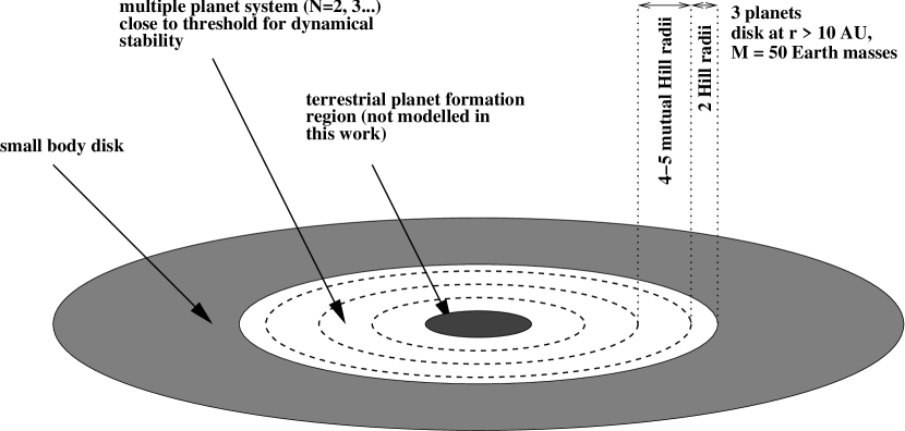
Figure 1.— Illustration of the initial conditions of our N-body simulations. Conceptually we envisage three radial zones: an inner terrestrial planet formation zone, an intermediate region in which gas and ice giants form, and an outer disk composed of small bodies that fail to form large planets prior to the dispersal of the gas disk. Our specific realization of this model assumes that three planets form with an orbital spacing that is close to the threshold for dynamical instability in the absence of an exterior disk. We additionally assume that the properties of the small body disk are fixed across systems, and do not model the terrestrial planet region.

We adopt a simple and well-defined version of the conceptual model shown in Figure 1 as the initial conditions for our scattering simulations. We assume that three planets form randomly separated by 4-5 mutual Hill radii $R_{H,m}$,

$$R_{H,m}=\frac{1}{2}\,(a_{1}+a_{2})\,\left(\frac{M_{1}+M_{2}}{3\,M_{\star}}\right)^{1/3}.$$ (1)

Here $a$ is the orbital semimajor axis, $M$ is the planetary mass, $M_{\star}$ is the stellar mass (fixed at 1 $M_{\odot}$), and subscripts 1 and 2 refer to the inner and outer planet, respectively. The spacing of 4-5 $R_{H,m}$, which is common across all but one of our sets of runs, was chosen to yield systems that are unstable on a $10^{5}-10^{6}$ year timescale (Chambers et al. 1996; Marzari & Weidenschilling 2002; Zhou et al. 2007; Chatterjee et al. 2008). The exception is our ensemble of runs with three $3\ M_{\rm J}$ planets, for which the number of unstable cases was so small that we adjusted the spacing to be 3.5-4 $R_{H,m}$ and re-ran the simulations (we still use the set of more widely-spaced, mostly stable simulations in our analysis of mean motion resonances in Section 4).

The outermost planet of the three planets was placed two (linear) Hill radii,

$$R_{H}=a\left(\frac{M}{3M_{*}}\right)^{1/3},$$ (2)

interior to 10 AU. We then chose a single random variable, uniformly distributed in the range between 4 and 5, to define the interplanetary spacing. The two additional planets were placed on the appropriate orbits, moving toward the (Solar-mass) star. Planets were given zero eccentricity and randomly-chosen mutual inclinations of less than 1 degree. We performed ten sets of simulations, varying the planetary mass distribution in each set. For our two largest sets (1000 simulations each) we randomly selected planet masses according to the observed distribution of exoplanet masses (Butler et al. 2006),

$$\frac{{\rm d}N}{{\rm d}M}\propto M^{-1.1}.$$ (3)

In the Mixed1 set we restricted the planet mass $M_{p}$ to be between a Saturn mass $M_{\rm Sat}$ and three Jupiter masses $M_{\rm Jup}$. For our Mixed2 set, the minimum planet mass was decreased to 10 ${\rm\,M_{\oplus}}$.

Although, strictly, we have little knowledge of the actual mass function of extrasolar planets at orbital radii beyond 5 AU, we regard the runs set up with the mass function observed at smaller radii as the most realistic. To gain additional insight into the behavior of more idealized systems, we performed four additional sets of simulations with equal mass planets (500 simulations each), and four sets that included radial mass gradients (250 simulations each). These sets are named with the appropriate planet masses, starting with the closest to the star outward; for example, in the 3J-J-S set the three Jupiter-mass ($3M_{\rm J}$) planet is closest to the star, followed by a Jupiter-mass planet and a Saturn-mass planet. The eight sets are: 3J-3J-3J, 3J-3J-3J, S-S-S, N-N-N, 3J-J-S, S-J-3J, J-S-N, and N-S-J, where $3J$ refers to a planet mass of $3M_{\rm J}$, $J$ is $M_{\rm J}$, $S$ is a Saturn mass $M_{\rm S}$, and $N$ is $30{\rm\,M_{\oplus}}$ (the “$N$” is intended to refer to Neptune, although the mass is augmented by just under a factor of two from Neptune’s true mass of 17 ${\rm\,M_{\oplus}}$ to maintain roughly a factor of three between the different planet masses).

Each of our $\sim$5000 simulations was run twice: once with just the three planets and once also including an external planetesimal disk. The simulations without disks were presented in Raymond et al. (2008a, 2009a) and are used in this paper only as a comparison sample. Simulations with disks included 1000 planetesimal particles distributed between 10 and 20 AU following a radial surface density profile $\Sigma\propto r^{-1}$, roughly consistent with sub-mm observations of outer disks around young stars (Andrews & Williams 2007). In all cases the total mass of the disk was $50\ M_{\oplus}$. We note that the inner edge of the disk lies interior to the radius where a test particle in the restricted 3-body problem would be stable, so the disk is in immediate dynamical contact with the outer planet.

2.2. Integration

Each simulation was integrated for 100 Myr using the hybrid integrator in the Mercury simulation package (Chambers 1999) with a 20 day timestep. There is the potential for significant numerical error in the integration for objects with small perihelion distances, which is usually manifested in terms of a secular increase in energy for close-in particles (Rauch & Holman 1999; Levison & Duncan 2000). With our timestep of 20 days, the conventional wisdom that at least 10 steps are required per orbit implies that we would expect to be able to resolve the orbit of a body at 0.67 AU. In fact, a more detailed test using a test particle being forced into the star by a giant planet via the Kozai mechanism shows that the integration error remains less than $10^{-4}$ down to a perihelion distance of about 0.4 AU.

We gauged the fidelity of the outcome of each of our simulations based on the simple energy criterion ${\rm d}E/E<E_{X}$, where $E_{X}$ is an energy threshold. For the simulations without disks we used the value of Barnes & Quinn (2004), who showed that $E_{X}=10^{-4}$ is adequate to test for dynamical stability of multi-planet systems. For the simulations with disks, the typical simulation error was actually ${\rm d}E/E\sim 10^{-4}$, even for cases in which the planets were stable and experienced very little orbital evolution. By sifting through a large number of examples and looking at the energy conservation of individual bodies, it appeared that an error threshold of $E_{X}\approx 10^{-3}$ was adequate to yield reliable results. We therefore set a threshold $E_{X}=5\times 10^{-4}$. Runs that failed to meet our energy criterion were either rerun or rejected. For the Mixed1 and Mixed 2 sets all runs with ${\rm d}E/E>E_{X}$ were re-run with smaller timesteps: 5 days for simulations with no planetesimal disks and 10 days for simulations with disks. Tests showed that limits of 5 [10] days sufficed to accurately resolve orbits down to perihelion distances of 0.15 [0.25] AU. In each set some of the re-run simulations (typically 15-35) still did not meet our energy criterion and were discarded from the sample. For the remaining sets of simulations our finite computational resources did not allow us to re-run those simulations with disks that failed the energy test. In these cases we discarded the examples with poor energy conservation based on the initial 20 day timestep runs. We do not believe that this introduced any substantial bias in our sample because certain expected outcomes occurred reliably; for example, the eccentricity distributions for the J-J-J and 3J-3J-3J simulations are virtually identical with and without disks.

2.3. Discussion of the initial conditions

Figure 2.— Location of the 2:1, 3:2, and 5:3 mean motion resonances (MMRs) for two planets in the parameter space of the sum of the two planets’ masses and their separation in mutual Hill radii (see Eq 1). Across a range of masses, the initial separations we consider often imply proximity to one of these resonances.

The details of our planetary initial conditions are motivated primarily by considerations of simplicity, and by the desire to pick planetary separations that are not grossly unstable. Our spacing of 4-5 $R_{H,m}$ would, however, be broadly consistent with models in which planets became temporarily trapped in mean motion resonances (MMRs) during the gaseous disk phase (Snellgrove et al. 2001; Lee & Peale 2002; Thommes et al. 2008b). Figure 2 shows the location of the 2:1, 3:2 and 5:3 mean motion resonances (MMRs) as a function of the summed mass of the planets involved. These are resonances that might be commonly populated during the gas disk phase, with the 5:3 MMR being generally unstable once the gas dissipates (Kley et al. 2004; Pierens & Nelson 2008). For a range of planet masses between 0.5 $M_{\rm J}$ and 5 $M_{\rm J}$, at least one of these resonances lies in the range probed by our simulations. We observe, of course, that a model based specifically on the idea of resonance trapping followed by release would differ in detail from ours, since in this case the planetary spacing in units of mutual Hill radii would correlate with the planetary masses.

Our choices of disk mass and radial extent are also somewhat arbitrary. A disk mass of 50 $M_{\oplus}$ is similar to that used in successful outer Solar System models, such as the Nice model (Gomes et al. 2005), and it is also comparable to the summed core masses that one would expect for three giant planets. It is thus roughly consistent with the idea that planetesimals in a disk with a continuous surface density distribution accreted to form cores inside some characteristic radius, while failing to do so further out. Our inner disk radius of 10 AU, on the other hand, is no more than a guess. It could typically be larger, in which case all of the disk-driven effects discussed in this paper would only be manifest for planets further out.

3. Statistical distribution of outcomes

Table 1Scattering Simulations

Set	N (no disks)	unstable–frac	N (disks)	unstable–frac
Mixed1	965	569 – 0.590	979	442 – 0.451
Mixed2	982	744 – 0.758	986	521 – 0.528
3J-3J-3J	368	241 – 0.655	152	55 – 0.362
J-J-J	452	232 – 0.513	380	96 – 0.253
S-S-S	390	362 – 0.928	324	196 – 0.605
N-N-N	357	355 – 0.994	212	142 – 0.670
3J-J-S	250	150 – 0.600	216	55 – 0.255
S-J-3J	245	219 – 0.894	229	147 – 0.642
J-S-N	250	206 – 0.824	247	43 – 0.174
N-S-J	245	221 – 0.902	177	148 – 0.836

Our initial conditions start with planets on orbits that are widely enough separated that few systems show substantial dynamical evolution on very short timescales ($10^{3}$ yr). On longer timescales the dynamical effect of the disk can be important, and either stabilize or destabilize the system against close encounters. To analyze our results, we separately consider the subsets of our runs that were “stable” versus those that were “unstable”. In this context, we define a stable system as one in which no close encounters between planets occurred over 100 Myr. A close encounter occurs when any two planets enter their mutual Hill sphere. An unstable system is thus one in which any two planets underwent at least one close encounter. Table 1 lists the fraction of each set of simulations that was stable with and without disks.

The above definition of stability, while precise and easily measured from the simulations, fails to capture the full range of behavior seen in runs with planetesimal disks. We therefore introduce a different classification in §3.3, where we consider how the characteristic timescale for evolution of the joint planet-disk system correlates with the presence of close encounters and architectural re-arrangement.

3.1. Instability Timescales

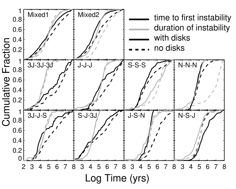
Figure 3.— Cumulative distributions of instability timescales for each set of simulations. Solid lines represent cases with disks, and dashed lines without disks. Note that the total planet mass increases to the left.

Given the spacing of 4-5 mutual Hill radii, we expect that the typical instability timescale in our simulations should be $10^{5}-10^{6}$ years (Mazari & Weidenschilling 2002; Chatterjee et al. 2008). Indeed, the median time for the first close encounter between planets in the cases without disks ranged from 58,000 years (S-S-S) to 3.1 Myr (3J-3J-3J). Instabilities typically set in earlier for systems containing less massive planets (see Chambers et al. 1996), and when the planet mass increases outwards (i.e., N-S-J simulations went unstable more quickly than J-S-N simulations).

Dynamically unstable systems tend to stabilize by destroying one or more planets, usually via collision with another planet or hyperbolic ejection. Systems with equal-mass planets tend to undergo far more close encounters over a much longer timespan than systems with significant mass differences between planets. The planets that survive in systems with equal-mass planets have much larger eccentricities than those in unequal-mass systems (Ford et al. 2003; Raymond et al. 2008a). The duration of instability is also mass-dependent: systems with low but equal-mass planets remain unstable for longer periods than systems in which the planet masses are scaled up.

Figure 3 shows the cumulative distribution of (1) the timescale from the start of each simulation to the first close encounter between planets (shown in black), and (2) the duration of the system instability, i.e. the time from the first to the last close encounter. We plot all ten sets of runs, both with and without planetesimal disks. For this unstable subset of runs, the 100 Myr duration of the simulations is sufficient to observe the onset and full duration of the instability in almost all cases.

With the sole exception of the N-S-J runs, the onset of instabilities in systems with disks occurs sooner than in those without disks (Fig. 3). One important effect of the presence of the planetesimal disks is clearly to stabilize systems that might otherwise be unstable on long timescales. This effect is most pronounced in systems with low-mass outer planets (e.g., the J-S-N cases). The reason for this is likely related to the mass dependence of the migration rate of a planet through a planetesimal disk, which is a strongly decreasing function of planet mass once the mass exceeds the mass of planetesimals within a few Hill radii (Ida et al. 2000; Kirsh et al. 2009). This migration can cause two planets (usually the outer two) to cross a low-order mutual mean motion resonance (see Fig 2). MMR crossings lead to an increase in planetary eccentricities (e.g., Chiang et al. 2002; Tsiganis et al. 2005), and trigger an instability that leads to close encounters.

Disks also reduce the duration of the unstable phase, but only in systems containing lower-mass outer planets. The most dramatic example are the N-N-N simulations, for which the typical period of close encounters was reduced by a factor of more than 100 (Fig. 3). This occurs because the orbits of high-eccentricity planets are circularized via dynamical friction with the planetesimal disk (e.g., Thommes et al. 1999), and this process is faster and more efficient for lower-mass planets. As scattered planets are re-circularized by the disk, their periastron distances are increased, they are removed from the region of scattering and future encounters between planets do not occur. In contrast, the planetary dynamics in systems with a massive planet adjacent to the planetesimal disk are effectively shielded from the effects of the planetesimal disk such that the duration of instabilities is the same as for simulations with no disks.

3.2. Characteristic Evolution

In planetary systems with no dissipation, once an instability occurs the endpoint is almost inevitably a violent event: a planet-planet collision, a planet-star collision, or a hyperbolic ejection from the system. However, in systems with dissipation from gaseous or planetesimal disks, the situation changes and the number of potential outcomes increases. The key new processes that arise from the presence of a planetesimal disk occur primarily for planets whose masses are similar to the planetesimal disk mass. Given our disk mass of 50 ${\rm\,M_{\oplus}}$, it is the simulations that include at least one roughly Saturn-mass or smaller planet that are affected. Interactions between the planetesimal disk and lower-mass planets can lead to angular momentum exchange and radial migration (Fernandez & Ip 1984). In addition, dynamical friction from the planetesimal disk can re-circularize the orbit of a scattered planet. Both of these processes feature prominently in recent models of the dynamical evolution of the Solar System’s giant planets (Malhotra 1995; Thommes et al. 1999; Tsiganis et al. 2005; Ford & Chiang 2007).

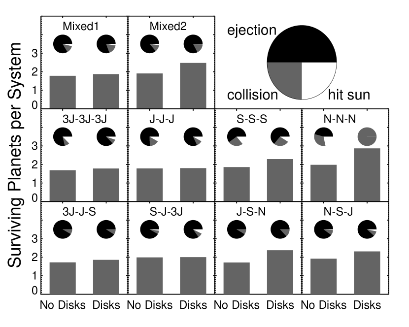
Figure 4.— A summary of the outcomes of our simulations. The bar graph in each panel shows the mean number of surviving planets per system for all cases that were unstable, with (right) and without (left) disks. The pie chart in each panel shows what happened to the destroyed planets in each case: ejection (black), planet-planet collision (gray), or collision with the star (white).

Figure 4 shows the range of outcomes of the unstable simulations for each giant planet configuration. The number of planets surviving per system increases for simulations with disks, but only for cases that contain a low-mass planet. The most dramatic difference is seen in the N-N-N simulations, for which the number of planets per unstable system increased from 1.98 to 2.87, meaning that only one out of every 7.5 unstable simulations with disks destroyed a planet. The pie charts in Fig. 4 show what happened to the destroyed planets in each case. For almost all cases, the dominant destruction mechanism was ejection from the system, which accounted for at least 3/4 of the destroyed planets in all configurations except S-S-S and N-N-N. In the N-N-N simulations without disks, ejection and collisions played a comparable role, which is not surprising given that the ratio of the escape speed from the planet to the escape speed from the planetary system (sometimes called the “Safronov number”, $\Theta$), is the smallest for any system, only about 2 (Ford et al. 2001; Goldreich et al. 2004). In the N-N-N simulations with disks, gravitational kicks during close encounters were not strong enough to eject a single planet in any simulation. The reason for this is twofold. First, dynamical friction efficiently circularizes the orbits of low-mass planets such that the typical encounter speed is low. Second, dynamical friction is also effective at effectively capturing scattered planets in the disk since the total disk mass actually exceeds the planet mass (30 ${\rm\,M_{\oplus}}$) in this case.

3.3. Timescales for Planet-Planetesimal Disk Interactions

We have seen that the planetesimal disk can have a strong influence on the planets’ dynamical evolution. The planets have a back-reaction on the disk itself, pumping up planetesimal eccentricities via dynamical friction and removing planetesimals from the system via dynamical ejection or collision. The number and strength of planet-planetesimal interactions depends most strongly on the planetary orbits. If the planets’ orbits remain circular then the planets can interact with only a fraction of the disk and encounter velocities depend mainly on the planetesimal eccentricities. If, however, planetary orbits are eccentric then the planets can interact with a larger fraction of the disk and encounter speeds will be larger, resulting in more frequent ejection of planetesimals. Thus, the perturbations felt by the planetesimal disk will correlate with the planetary orbits and therefore the dynamical stability of the planets.

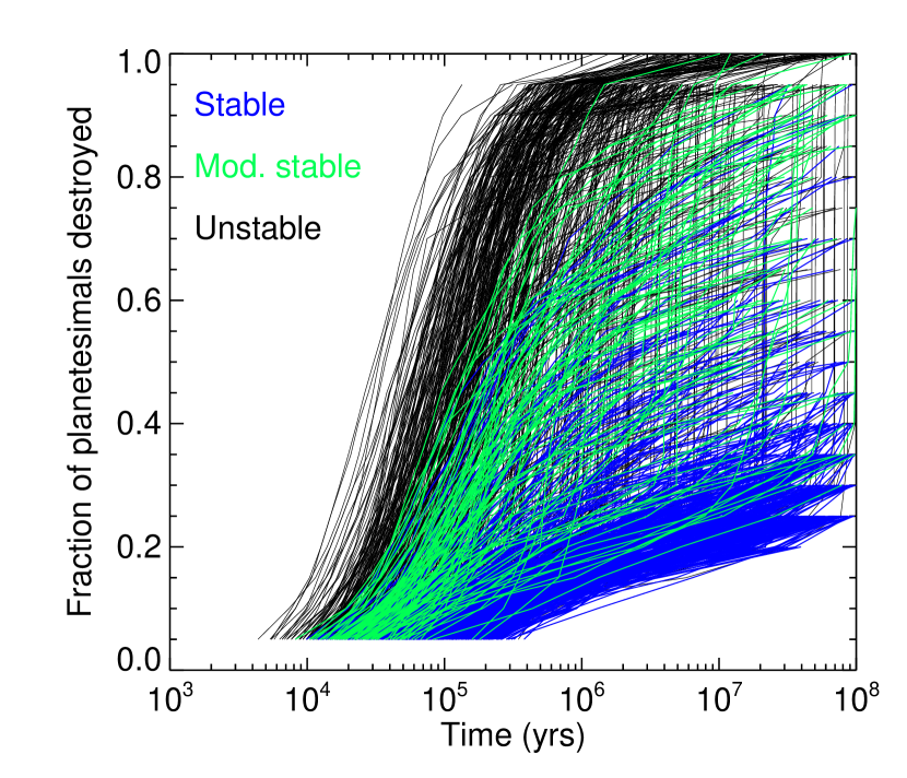
Figure 5.— Timescale for the destruction (via hyperbolic ejection, collision with a planet or collision with the central star) of the planetesimal disk for the Mixed1 simulations. Black lines correspond to unstable simulations which had at least one close encounter between planets. Green lines refer to “moderately stable” simulations which experienced no planetary close encounters but the final planetary system had a mass-weighted eccentricity larger than 0.025. Blue lines correspond to “stable” simulations, which experienced no close encounters between planets and remained on low-eccentricity orbits. Note that we only plot every 5% of planetesimals destroyed.

Figure 5 shows the timescale for the destruction of a given fraction of the planetesimal disk for all of the Mixed1 simulations, where each curve corresponds to a single simulation. Here we have subdivided the “stable” simulations, which never experience close encounters, into moderately stable and stable subsets. We define a moderately stable system as one which never experienced a close encounter between planets but for which the final mass-weighted planetary eccentricity is larger than 0.025. These systems have thus experienced significant planet-planet perturbations despite the absence of close planetary encounters.

The unstable Mixed1 systems destroy the majority of their planetesimal disks on a $10^{5}-10^{6}$ year timescale (Fig. 5), although late-onset instabilities can be seen as nearly vertical lines at later times. There is often a delay for the destruction of the last 10% of planetesimals because in most cases these have large inclinations such that the close encounters with the planets needed to reach zero energy are less frequent. In fact, many unstable cases do not destroy the entire planetesimal disk. Moderately stable systems can have a range in the timescale and amount of planetesimal destruction depending on the planet masses and evolution. For relatively massive planets, the sudden eccentricity increase that accompanies a resonance crossing leads to a corresponding jump in the eccentricities of many or most disk particles, leading to orbit crossings, close encounters and ejection. For less massive planets secular perturbations are weaker so less of the disk is destabilized during such events. One configuration that is quite efficient at clearing out planetesimals is a lower-mass outer planet and a high-mass middle planet. The outer planet’s low mass allows it to migrate outward somewhat due to planetesimal scattering. The scattered planetesimals, in turn, are quickly ejected by encounters with the high-mass middle planet.

The stable Mixed1 systems, which are relatively high-mass, destroy only a relatively small portion of the planetesimal disk. The outer planet interacts directly with planetesimals within the stability boundary and also may excite planetesimals that happen to be in resonances onto planet-crossing orbits. These directly-interacting planetesimals can be ejected by the outer planet or can be “passed” inward to interact with the inner planets, which typically eject the planetesimals. Thus, the inner planetesimal disk is quickly cleared out and interactions between the planets and the planetesimal disk become infrequent, with 50-75% of the disk remaining.

The evolution of the planetesimal disks in our simulations offers a rich data set to understand the connection between planetary dynamics and disk structure. In a future paper, we will correlate the planetary and planetesimal components of each system and calculate the infrared detectability of these disks for each case. For the remainder of this paper, we restrict ourselves to the planetary dynamics.

3.4. Eccentricity Distributions

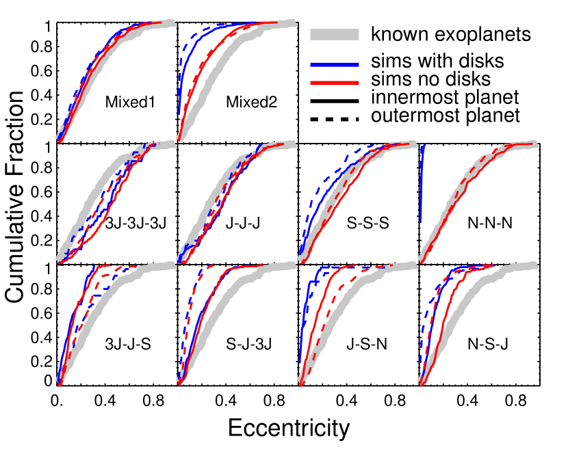
Figure 6.— Cumulative eccentricity distributions for the unstable simulations from each of our ten simulation cases, with (blue) and without (red) planetesimal disks, compared with the observed extra-solar systems exterior to 0.1 AU (thick grey line). The innermost planet from each simulation is shown with the solid lines, while the outermost planet is shown with the dashed lines.

Figure 6 shows the cumulative eccentricity distributions for the innermost and outermost planets in all of our unstable simulations, with and without disks. We also plot the observed exoplanet eccentricity distribution, excluding planets inside 0.1 AU which are likely to have had their orbits altered by tides (Jackson et al. 2008). We note that, since our simulations start with planets at fairly large radii, we do not populate the full radial range across which the observed distribution is determined. Currently, however, the evidence for any radial dependence to the eccentricity distribution is marginal (Ford & Rasio 2008), so the comparison between the observed and simulated distributions is justifiable.

Although the result is now well-established (Chatterjee et al. 2008; Jurić & Tremaine 2008), it is still startling to see from Fig. 6 how easily planet-planet scattering can reproduce the observed eccentricity distribution. With just the simple assumption that planets have the observed mass distribution and form on marginally unstable orbits (i.e., the Mixed1 simulations), we can produce a statistical match to the observed distribution. The planet-planet scattering model appears to be a very robust and simple way to explain the observed systems.

As expected, the difference between planetary eccentricities for simulations with and without disks is strongly mass dependent and clearly seen in a comparison between the Mixed1 and Mixed2 simulations. The effect of the planetesimal disk is clear for $M_{p}\lesssim M_{\rm S}$, and for the lowest-mass case, N-N-N, orbital re-circularization from planet-planetesimal disk interactions is so strong that there are no high-eccentricity planets at all – the most eccentric planet in all the N-N-N simulations with disks is just 0.06. As seen in previous work, scattering among equal-mass planets produces larger eccentricities than scattering among planets with different masses (Ford et al. 2003; Raymond et al. 2008a), and this is clearly seen in Fig. 6.

Variations between the eccentricities of inner and outer planets are caused by two different effects: scattering from other planets and eccentricity damping from the planetesimal disk. For the Mixed1 simulations there is very little difference between the inner and outer eccentricity distributions because there is no planetary mass gradient and the planet masses are too large to be significantly affected by the planetesimal disk. For the Mixed2 simulations with disks, outer planets have lower eccentricities. This offset is not seen for the simulations without disks. Thus, the lower-eccentricity outer planets are due to damping from the planetesimal disk. For simulations with equal-mass planets, there is a modest inner vs. outer eccentricity difference because of disk damping but only for the S-S-S cases, as the Jupiter-mass planets (J-J-J) barely feel the disk and 30 ${\rm\,M_{\oplus}}$ planets (N-N-N) are all quickly circularized. For systems with radial gradients in planet mass there is an inner vs. outer eccentricity difference caused by the simple mass-dependence of the recoil velocity during a planetary encounter. During instabilities involving different-mass planets, this leads to more massive planets having smaller eccentricities than less massive planets. For systems with negative mass gradients (3J-J-S and J-S-N), this causes the outer planets to have higher eccentricities than the inner planets, and the effect is reversed for systems with positive mass gradients (S-J-3J and N-S-J). For the lower-mass cases with mass gradients (J-S-N and N-S-J), the effects of preferential eccentricity damping of outer planets by the planetesimal disk are also clearly seen.

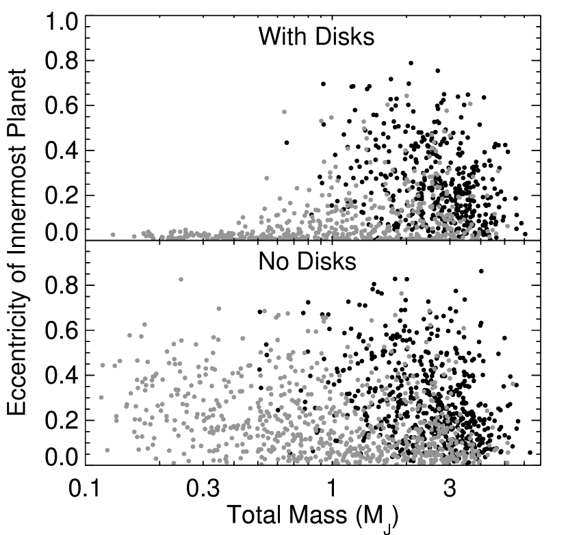
Figure 7.— Final eccentricity of the innermost planet vs. the total mass in surviving planets for the unstable Mixed1 (black) and Mixed2 (grey) simulations, with (top panel) and without (bottom panel) planetesimal disks. Disks result in a sharp transition to a low-eccentricity regime for system masses below about one Jupiter mass. For higher system masses, the observed exoplanet eccentricity distribution is recovered irrespective of the presence or absence of disks.

In Figure 7 we show the eccentricity of the innermost (and thus most easily detectable) planet as a function of the final total mass of the planetary system, using just the Mixed1 and Mixed2 simulations. In the presence of disks there is a strong correlation between these quantities (Raymond et al. 2009b). For systems with total masses of less than $\sim 1\,M_{\rm J}$, circular or near-circular orbits dominate. For higher system masses, on the other hand, planetary eccentricities display a large range, from near zero to $>0.8$. This correlation is much weaker if we plot, instead, planetary eccentricity against individual planet mass for all surviving planets (Figure 8). As is obvious from the cumulative distributions, disks do act to circularize low mass planets more than high mass planets, but there is no sharp transition between the two regimes. We interpret this difference as being due to the fact that it is the total mass of the planetary system that determines the disk lifetime and the ability of the disk to damp eccentricities, rather than any individual planet mass (see discussion in §3.6 below).

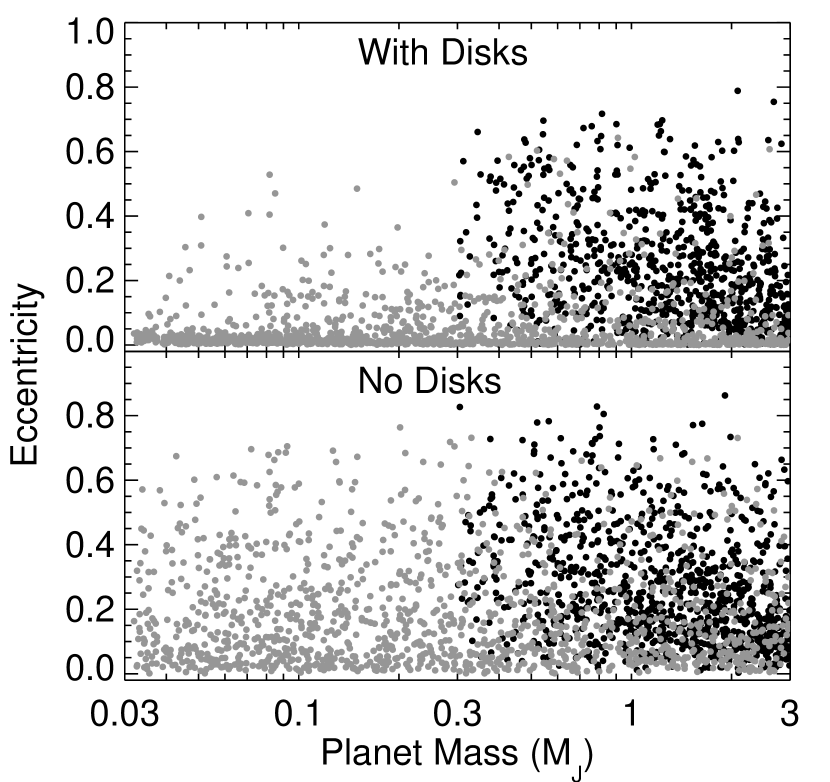
Figure 8.— Planetary eccentricity vs. mass for all surviving planets in the unstable Mixed1 (black dots) and Mixed2 (grey dots), with (top panel) and without (bottom panel) planetesimal disks.

3.5. Detectability of a transition to low $e$ at large orbital radii

The semi-major axis, beyond which our model predicts a transition to low eccentricity orbits for $M<M_{\rm J}$ planets, depends upon the characteristic inner radius of the primordial planetesimal disk (note that the mass at which the transition occurs will also vary with this quantity). This is a free parameter, which we have fixed at 10 AU. If, in reality, planetesimal disks do typically extend in to about 10 AU, our results suggest that the transition to the low eccentricity regime may be observable with feasible extensions of existing radial velocity surveys (if the inner extent of planetesimal disks is at substantially larger radii astrometry or direct imaging may offer better prospects). To quantify this, we have calculated the radial velocity amplitude $K$,

$$K=\frac{1}{\sqrt{1-e^{2}}}\left(\frac{M}{M_{*}}\right)\sqrt{\frac{GM_{*}}{a}}\sin i,$$ (4)

for the innermost surviving planet for all of the Mixed1 and Mixed2 runs. The distribution of $e$ as a function of $K$ is shown in Figure 9, assuming $M_{*}=M_{\odot}$ and (for simplicity) that $\sin i=1$. Since the detectability of a planet via radial velocity measurements depends upon the period as well as the amplitude, the points are further coded to indicate relatively short period ($P<2000\ {\rm days}$), intermediate period ($2000\ {\rm days}<P<4000\ {\rm days}$), and long period ($P>4000\ {\rm days}$) planets.

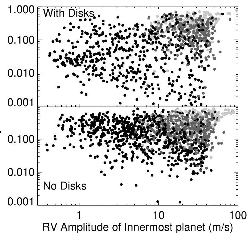
Figure 9.— The predicted signature of the transition to low eccentricity orbits in radial velocity surveys. The eccentricity of the innermost surviving planet is plotted as a function of the stellar radial velocity amplitude $K$ for the Mixed1 and Mixed2 simulations both with and without disks. The light, intermediate, and dark grey points correspond to planets with orbital periods $P<2000\ {\rm days}$, $2000\ {\rm days}<P<4000\ {\rm days}$, and $P>4000\ {\rm days}$, respectively. Detection of the dynamical influence of planetesimal disks requires either long duration (in excess of 10 years) monitoring sensitive to planets with $K<10\ {\rm m\ s}^{-1}$, or highly accurate determinations of the eccentricity of planets on almost circular orbits.

A measurement of $e(K)$ for the innermost planet provides no information as to the total mass of the planetary system, and as a consequence the transition to lower eccentricities at lower $K$ resembles that shown in Figure 8 ($e$ as a function of individual planet mass) rather than the sharper transition seen in Figure 7 ($e$ as a function of the final total system mass). Nonetheless, we see a clear trend to lower eccentricities that sets in for radial velocity amplitudes $K\lesssim 10\ {\rm m\ s}^{-1}$. Although there are high $e$ outliers at all values of $K$, for $K=1-5\ {\rm m\ s}^{-1}$ the typical eccentricity lies in the $10^{-2}-0.1$ range, whereas for $K>10\ {\rm m\ s}^{-1}$ values $e>0.1$ are obtained. Comparing the results with and without disks makes clear that this difference is caused by the damping effects of planetesimals.

Detection of planets with radial velocity amplitudes $K<10\ {\rm m\ s}^{-1}$, although not easy, is already possible (almost 40 such systems are currently known). The primary obstacle to observational study of the outer planet region, where the dynamical effects of planetesimal disks should become evident, is rather the long periods of planets. As is clear from Figure 9, essentially all of the low mass planets, whose orbits have been partially circularized by interaction with planetesimals, have periods in excess of 4000 dy. High precision radial velocity measurements, capable of finding planets with $K\approx 5\ {\rm m\ s}^{-1}$ and periods in excess of 10 years, are therefore required in order to start probing the dynamics discussed in this paper.

Inspection of Figure 9 suggests a second observational signature of planetesimal disk dynamics: the existence of extremely low eccentricity planets. In the presence of disks, a small but measureable fraction of even massive planets (with $K=10-30\ {\rm m\ s}^{-1}$) end up with $e<10^{-2}$, whereas such systems are rare in the absence of disks. Extremely precise measurements of eccentricity, capable of detecting an excess (above the predictions of pure scattering models) of truly circular orbits, would therefore be valuable even if such observations were only available for massive planets. The interpretation of an excess of circular orbits, however, would likely be more ambiguous than a measurement of the full $e(K)$ distribution, since it could reflect small amounts of gas damping or an admixture of systems that only formed one planet, as well as the dynamical influence of planetesimals.

3.6. Inclination Distributions

Planet scattering can lead to large mutual inclinations between the surviving planetary orbits, as well as misalignment with respect to the initial plane of the planets (Chatterjee et al. 2008; Jurić & Tremaine 2008). Mutual inclinations between the orbital planes of planets in multi-planet systems can be detected via astrometry (e.g., Bean & Seifahrt 2009), while any misalignment between the orbital plane and the plane perpendicular to the stellar spin axis can be detected directly for transiting planets via the Rossiter-McLaughlin effect (Gaudi & Winn 2007; Winn et al. 2005). Another interesting consideration is that the initial planetary plane coincides with the plane of the planetesimal disk and presumably also with the plane of the dust disk that should be produced by collisional grinding of planetesimals (e.g., Wyatt 2008).

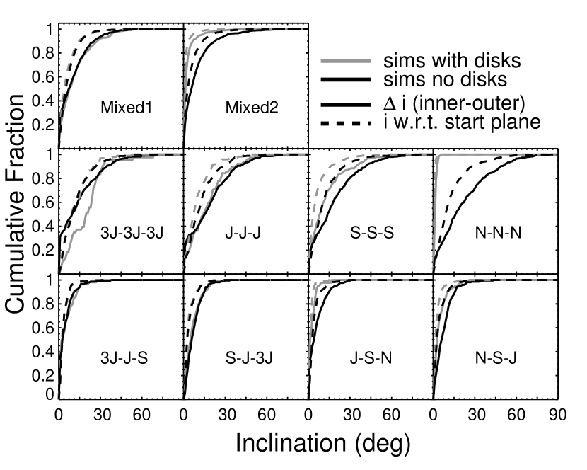
Figure 10.— Cumulative inclinations distributions for the unstable simulations from each of our ten simulation cases, with (blue) and without (red) planetesimal disks. The solid lines show the distribution of the mutual inclination between the orbits of the inner and middle planets for systems with two surviving planets. The dashed lines show the distribution of inclinations with respect to $i=0^{\circ}$, the initial plane of the planets and planetesimals.

Figure 10 (dashed lines) shows the distribution of inclinations with respect to the initial orbital plane for the unstable systems in all ten sets of simulations, both with and without planetesimal disks. As was the case for eccentricities, larger inclinations are generated in systems with equal-mass planets than in systems with large mass ratios. Inclinations in the few to $\sim$15 degree range are common in most sets of simulations, but only the equal-mass systems are able to generate larger inclinations. Unlike the eccentricity distributions for which higher-mass planets have higher eccentricities, all four equal-mass systems (without disks) have virtually identical inclination distributions.

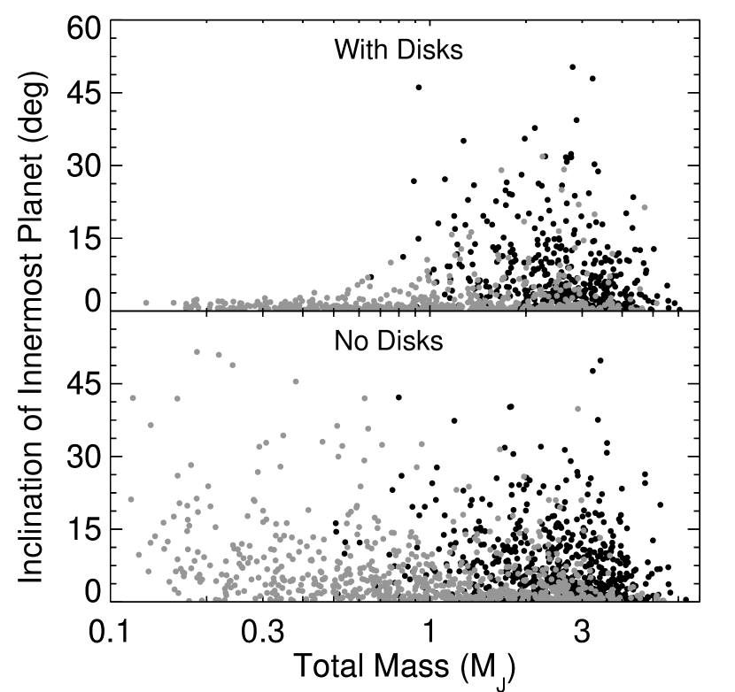
Figure 11.— The inclination of the innermost planet with respect to the initial orbital plane as a function of the total mass in surviving planets for the Mixed1 (black dots) and Mixed2 (grey dots) simulations.

As expected, the simulations with disks yielded smaller inclinations than the simulations without disks, and the effect was stronger for lower-mass planets. Figure 11 shows the inclination of the innermost planet, which as in the case of eccentricity is controlled by the total planetary mass rather than the individual planet masses. The same sharp break at $M_{tot}\approx 1M_{\rm J}$ is seen to divide planets with small inclinations vs. those with a large range in inclination.

The mutual inclination $\Delta i$ between two planetary orbits with inclinations $i_{1}$ and $i_{2}$ is given by:

$$\cos{\Delta i}=\cos{i_{1}}\cos{i_{2}}+\sin{i_{1}}\sin{i_{2}}\cos{\left(\Omega_{1}-\Omega_{2}\right)},$$ (5)

where $\Omega_{1}$ and $\Omega_{2}$ refer to the longitudes of ascending node. Figure 10 shows the distributions of the mutual inclination $\Delta i$ between the innermost and the adjacent planet in unstable systems for which two or more planets survived (solid lines). The $\Delta i$ values are consistently larger than the inclinations with respect to the initial orbital plane. During a close planetary encounter, if one planet is scattered in the $\hat{z}$ direction, then the other planet must receive a kick in the $-\hat{z}$ direction. For a single encounter that dominates the planets’ motion in the vertical direction, such a kick would also cause the two planets’ longitudes of ascending node to be offset by roughly 180^∘, depending on their eccentricities. Thus, the instantaneous mutual inclination will be close to the sum of the two planets’ inclinations with respect to their initial plane (Eq. 5). Although the alignment of the two planets’ nodes will change in time due to secular perturbations, angular momentum conservation requires that the mutual inclination remain relatively large.

As for the case of inclination with respect to the initial orbital plane, equal-mass planets yield much larger $\Delta i$ values than planets with large mass ratios. However, in this case the lower-mass equal-mass systems have higher mutual inclinations than the higher-mass cases. Ten percent of the unstable planets in the equal-mass systems without disks had inclinations larger than 35^∘ (3J-3J-3J), 39^∘ (J-J-J), 42^∘ (S-S-S), and 49^∘ (N-N-N), compared with 26^∘ for the Mixed1 simulations. The larger inclinations in lower-mass equal-mass planetary systems are caused by the ease with which the high-mass planets can eject each other. The higher-mass systems for which two planets survive have undergone far fewer close encounters than the lower-mass systems with two surviving planets: the median number of encounters in the unstable 3J-3J-3J, J-J-J, S-S-S, and N-N-N systems for which two plants survived was 81, 175, 542, and 1871, respectively. However, the mass-weighted eccentricities of the two-planet equal-mass systems were slightly higher for the higher-mass planets. Thus, large planetary eccentricities are linked with the strength of encounters between planets while large inclinations are linked with a large number of scattering events. Note that the number and strength of close encounters in systems with significant mass ratios is far less, thus explaining their lower eccentricities and inclinations (see Raymond et al. 2009a).

As seen in Fig. 3, the duration of the close encounter phase (as well as the total number of encounters) is reduced for the simulations with planetesimal disks. Therefore, we expect lower inclinations for simulations with planetesimals – this is indeed clearly seen in Fig. 10. The extreme damping for the N-N-N simulations is again seen in terms of their very low inclinations and mutual inclinations in systems with planetesimal disks.

3.7. An angular momentum argument for the transition mass

What sets the boundary between typically eccentric (and inclined) and typically circular (and coplanar) planets, which we have determined empirically lies at a total system mass of about $M_{\rm tot}\approx 0.7\ M_{\rm J}$? Plausibly, this transition mass may be set simply by the reservoir of disk angular momentum that is able to interact with the planet and circularize its orbit.

To illustrate the point, we construct an (over)-simple model of the circularization process. Let us assume that scattering (with or without disks) typically yields a single planet with some characteristic semi-major axis $a$, eccentricity $e$, and inclination $i$. The orbital angular momentum deficit ($AMD$) quantifies the difference between the orbital angular momentum for a circular orbit as compared to an eccentric and inclined one at the same semi-major axis. The $AMD$ is given by,

$$AMD=M\sqrt{GM_{*}a}\left(1-\cos i\sqrt{1-e^{2}}\right).$$ (6)

To fully circularize the planet, we need to add this much angular momentum via planetesimal interactions. If these interactions occur primarily at or near apocenter in a disk with surface density profile,

$$\Sigma=Cr^{-1},$$ (7)

with $C$ being a constant, the mass of the disk within a radial zone of half-width $n$ Hill radii (at the apocenter distance) is,

$$\Delta M_{\rm disk}=4\pi nC\left(\frac{M}{3M_{*}}\right)^{1/3}a(1+e).$$ (8)

Assuming the planetesimals to have circular orbits, the total angular momentum of the disk that interacts with the planet is, approximately,

$$\Delta L_{\rm disk}\simeq\Delta M_{\rm disk}\sqrt{GM_{*}a(1+e)}.$$ (9)

By equating the available angular momentum to the angular momentum deficit, we find that the disk can circularize planets for masses,

$$M\lesssim\frac{(4\pi nC)^{3/2}}{(3M_{*})^{1/2}}\frac{(1+e)^{9/4}}{(1-\cos i\sqrt{1-e^{2}})^{3/2}}a^{3/2}.$$ (10)

This is an analog of the usual isolation mass, except here in the case of circularization rather than accretion. One should note that the factor involving $e$ is not of order unity – typically it is quite large ($\sim 10^{2}$).

This analysis is quite crude, but it does predict transition masses that are of the same order of magnitude as those observed. For example, substituting our disk parameters and adopting planetary orbital elements of $a=8\ {\rm AU}$, $e=0.4$ and $i=10^{\circ}$, we obtain (for $n=2$) a transition mass $M\approx 0.6\ M_{\rm J}$. This suggests that we should interpret the transition mass as being a consequence of the finite angular momentum, within the disk, available to circularize planets. So, why is it that the eccentricity is controlled by the total planet mass rather than the individual planet mass (e.g., Figs. 7 and 8)? The answer appears to be that it is the total mass which regulates the eccentricity excitation, which in turn determines the amount of damping by scattering disk particles.

3.8. Radial Mass Distributions

Planet-planet scattering tends to segregate systems by mass, with more massive planets closer-in and less massive planets farther out (Chatterjee et al. 2008). We expect this effect to be magnified in systems with planetesimal disks because the disk can “trap” low-mass planets that would otherwise be ejected from the system. To look at the radial mass evolution of our simulations we restrict ourselves to the Mixed1 and Mixed2 cases which did not start with pre-defined radial mass gradients.

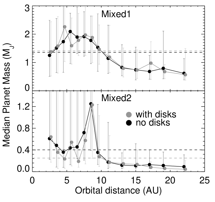
Figure 12.— Radial mass distribution of scattered planets for the Mixed1 and Mixed2 simulations, with (grey) and without (black) planetesimal disks. The dots represent the median planet mass in a given radial bin, and the error bars show the 10% to 90% range in values. The point at 22 AU includes all planets beyond 20 AU. The dashed horizontal lines show the median planet masses for the ensemble of all scattered planets in a given set. Note that the simulations with disks are offset by 0.2 AU for clarity.

Figure 12 shows the median planet mass as a function of orbital distance for the unstable Mixed1 and Mixed2 systems, with and without disks (also shown is the 10-90% range of planet masses in a given radial bin). For the Mixed1 systems, there is a clear segregation of high-mass planets to the inner system and low-mass planets in the outer system, with very little difference for the simulations with and without planetesimal disks. The most massive planets tend to reside at 4-9 AU, close to the starting initial orbits.

Radial mass segregation is also clear in the Mixed2 simulations but there are additional subtleties. As for the Mixed1 cases, high-mass planets are confined within 10 AU and low-mass planets outside 10 AU. There is a large peak in the median Mixed2 planet mass between 8 and 9 AU both with and without planetesimal disks. There are actually 2-3 times more planets in this 1 AU-wide bin than in adjacent bins for the Mixed2 simulations with and without disks. Perhaps surprisingly, any differences in mass segregation caused by disks appear to be modest even for the Mixed2 simulations.

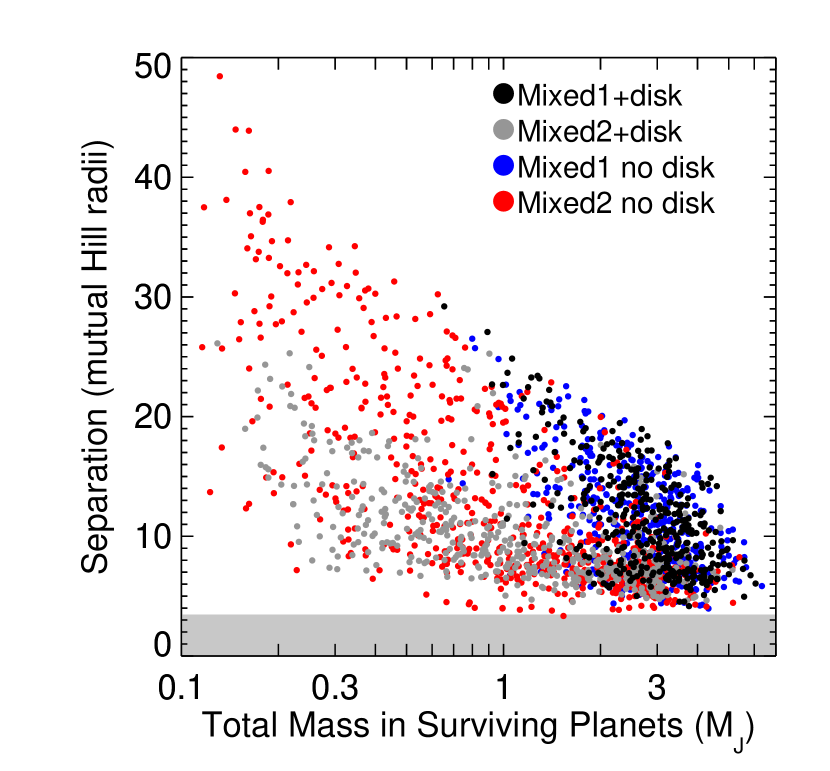
Figure 13.— Final planetary separation in units of mutual Hill radii for unstable Mixed1 and Mixed2 simulations, with (black and grey) and without (blue and red) planetesimal disks. Only systems with two or more surviving planets are shown – for systems with three surviving planets only the separation between the inner two planets is included. The shaded horizontal line shows the two-planet stability limit of $3.46R_{H,m}$ (Marchal & Bozis 1982; Gladman 1993).

Scattering tends to spread planetary systems out. We can quantify this by looking at the planetary separations at the end of the simulations in units of mutual Hill radii $R_{H,m}$ (recall that all simulations started separated by 4-5 $R_{H,m}$). Figure 13 shows the separation of the two inner planets as a function of the total mass in surviving planets for the Mixed1 and Mixed2 simulations, with and without disks. There are several interesting pieces of information in Fig. 13. First, the typical interplanetary spacing is $\sim$ 4-30 $R_{H,m}$, showing that most systems have indeed spread out. Second, the interplanetary spacing decreases significantly for larger system masses, although there remains a large spread for any given mass. This general trend can be explained by the much larger number of scattering events undergone by lower-mass systems before the destruction (usually by ejection) of a planet. The spread in separation is due in part to stochastic variations in scattering events from simulation to simulation and in part to variations in planetary mass ratios – the larger number of scattering events for equal-mass systems causes them to be more widely-spaced than systems with larger mass ratios. Third, there is an abrupt break between the separations of lower-mass systems with and without planetesimal disks. For $M_{tot}\lesssim 0.7M_{\rm J}$, systems with disks are much more compact than systems without disks. This is a result of the damping of the planetesimal disk: low-mass planets on wide orbits have their eccentricities efficiently damped and their perihleion distances increased such that they avoid additional close encounters with the inner planet. This is evidenced by the fact that the break between the simulations with and without disks occurs at the same total planet mass as for the eccentricity and inclination distributions (see Figs 7 and 11).

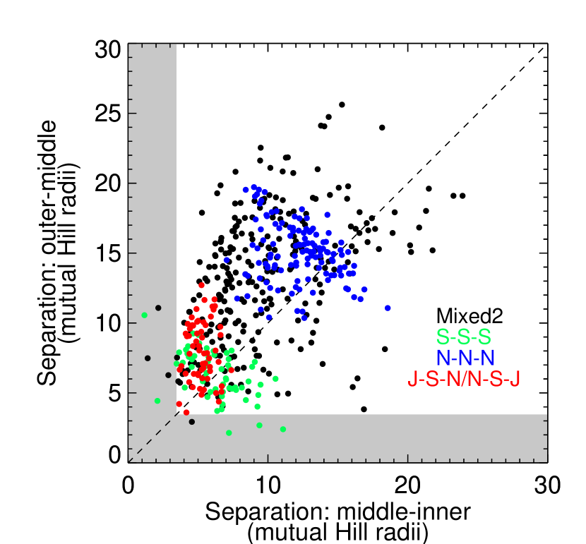
Figure 14.— For scattered systems with three surviving planets, the separation of the outer planet pair ($y$ axis) vs. the inner planet pair ($x$ axis), in units of mutual Hill radii. Five sets of simulations are shown in different colors. The shaded horizontal and vertical lines shows the two-planet stability limit of 3.46 $R_{H,m}$.

For systems in which three planets survive, the outer two planets tend to be more widely spaced than the inner two. Figure 14 shows the separation of each pair of planets for unstable systems which preserved all three planets. In the bulk of cases the outer pair of planets are indeed more widely-spaced than the inner pair. However, there do exist many cases for which the outer planets are more compact, as well as a few cases in the Hill unstable region which are likely to be unstable on slightly longer timescales. Systems with a more compact outer pair of planets tend to be those with lower-mass middle planets. As the outer planet scatters planetesimals inward, a massive middle planet can eject them from the system, causing the planet to move inward and leading to a compact inner system but a spread out outer system. In contrast, a low mass middle planet cannot generally eject the scattered planetesimals and so simply scatters them toward the inner planet, causing the middle planet to move outward, yielding a compact outer system and a more spread out inner system.

3.9. Planets at large orbital separations

Planet-planet scattering creates a population of high-eccentricity planets with large apocenter distances (Veras et al. 2009; Scharf & Menou 2009). For the vast majority of cases, these planets, which can have semimajor axes as large as $\gtrsim 10,000$ AU, represent a transient phase on the path to dynamical ejection. These planets are of interest because they represent the source of so-called “free-floating planets”. In some cases their large separations mean that they could be good targets for direct detection, although they probably only exist for the first 10-100 Myr of a star or star cluster’s lifetime.

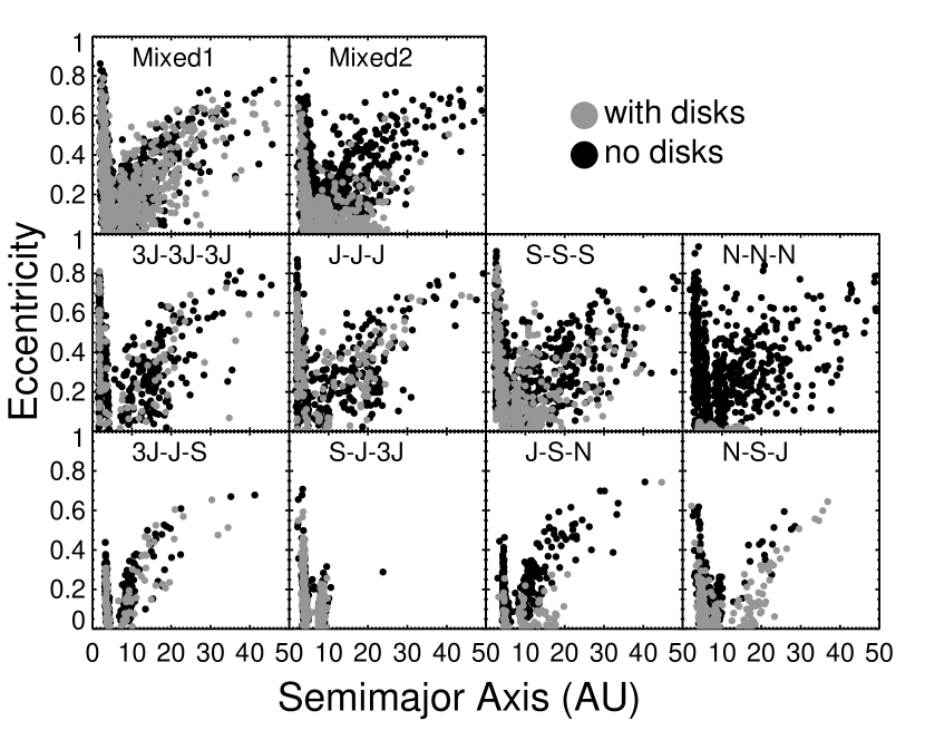
Figure 15.— Orbital eccentricity vs. semimajor axis of scattered systems with (in grey) and without (in black) planetesimal disks, for each of our ten initial mass distributions.

In our simulations we imposed an ejection radius of 100 AU, so we were unable to probe very distant planets. Nonetheless, we can study planets that ended up on transient, or in some cases stable, orbits beyond the initial radial extent of our initial conditions. To address the issue of planets on widely-separated orbits, we kept track of the time spent by each planet in each simulation with an aphelion distance in radial bins of 25-50 AU, 50-75 AU, and 75-100 AU. We also characterized planets in each of those bins as either being in a transitional state (usually on the path to ejection) or on stable orbits. Inspection of the final eccentricity as a function of semi-major axis distributions, plotted in Fig. 15, shows immediately that a large number of scattered planets survived on stable orbits with large aphelion distances.

Table 2Scattered planets at large orbital distances (aphelion $Q>25[50]$ AU)^⋆

	No Disks			With Disks
Set	frac stable	frac trans.	$\langle t\rangle$ (Myr)	frac stable	frac trans.	$\langle t\rangle$ (Myr)
Mixed1	0.14 [0.03]	0.44	0.64 [0.10]	0.17 [0.03]	0.45	0.92 [0.15]
Mixed2	0.15 [0.03]	0.59	2.55 [0.54]	0.03 [0.00]	0.23	0.46 [0.03]
3J-3J-3J	0.23 [0.05]	0.23	0.69 [0.01]	0.29 [0.07]	0.29	2.60 [0.01]
J-J-J	0.29 [0.06]	0.49	0.77 [0.03]	0.29 [0.04]	0.53	1.88 [0.02]
S-S-S	0.34 [0.07]	0.64	1.36 [0.28]	0.18 [0.04]	0.46	2.19 [0.28]
N-N-N	0.32 [0.08]	0.63	7.58 [1.69]	0.00 [0.00]	0.00	0.00 [0.00]
3J-J-S	0.06 [0.01]	0.31	0.67 [0.08]	0.11 [0.04]	0.29	0.19 [0.01]
S-J-3J	0.00 [0.00]	0.14	0.01 [0.01]	0.00 [0.00]	0.11	0.01 [0.00]
J-S-N	0.13 [0.02]	0.59	1.99 [0.33]	0.05 [0.02]	0.33	2.45 [0.66]
N-S-J	0.05 [0.00]	0.59	0.16 [0.06]	0.12 [0.03]	0.41	1.30 [0.14]

^⋆ The first column (“frac stable”) represents the fraction of scattered systems containing a planet on a long-term stable orbit with aphelion distance $Q$ larger than 25 [50] AU. The second column (“frac trans”) shows the fraction of scattered systems for which at least one planet spent at least one output interval of $10^{5}$ years with $Q>25$ AU during a transitional ejection phase. The third column shows the mean time $\langle t\rangle$ in Myr during which a planet had $Q>$ 25 [50] AU for the transitional systems. Note that $\langle t\rangle$ is averaged over all scattered systems, including a fraction that did not undergo a transitional outer planet phase.

Table 2 shows the statistics of planets at large orbital separations in our simulations. The table includes information about both stable and transitional planets with aphelion distances $Q>25$ AU and $Q>50$ AU. First of all, we see that scattering among equal-mass planets is far more efficient at producing stable planets with large orbital radii than scattering among planets with mass gradients. This is simply because of the much larger number of scattering events that occur in equal-mass systems. Next, we see that this trend does not hold for the fraction of systems which experience a transitional, high-$Q$ phase. Lower-mass planets have a higher probability of experiencing this transitional phase. We interpret this as an ejection timescale issue – the number of encounters and duration of the instability phase increases dramatically for lower-mass systems (see Section 3.1) such that the typical ejection is very drawn out. In contrast, for higher-mass planets a smaller number of scattering events is needed to eject a planet. Our analysis only includes outputs every $10^{5}$ years; thus, ejections which occur in less than that time are not registered or counted in Table 2. For equal-mass and mixed systems, the mean time during our 100 Myr simulations for which a planet could be observed with $Q>$ 25 [50] AU correlates with the fraction of transitional systems, with typical observable probabilities of a couple of percent (the probability is here calculated as $\langle t\rangle$ divided by the 100 Myr simulation length). For the mass gradient simulations, $\langle t\rangle$ is longer for negative mass gradients (for 3J-J-S and J-S-N). This is because the most massive planet is closer-in in those cases, deeper in the star’s potential well, such that a larger number of encounters is needed to reach the system’s escape velocity.

As expected, the higher-mass systems are barely affected by the presence of planetesimals disks in terms of the fraction of orbits which are at large distances and the fraction that appear in the transitional phase. However, the duration of the transitional ejection phase is lengthened by a factor of a few for the equal-mass cases, meaning that the time required to eject those planets is increased due to the damping from the disk. For the lower-mass planets there are fewer planets at large orbital distances in terms of both stable and transitional configurations. This is simply due to the disk’s ability to “trap” planets by orbital circularization. This circularization occurs within the disk, so trapped planets are generally confined to orbits within the outer edge of the disk, at 20 AU.

Can observations of long-period planets tell us anything about the inner planets that spawned them? Assuming that outer planetesimal disks are ubiquitous, equal-mass and higher-mass planetary systems are more likely to populate distant stable orbits than lower-mass systems or those with large mass ratios between planets. However, a wide range of configurations produces long-lived transient planets on large orbits that are generally on their way towards dynamical ejection. We suspect that combining observations of long-period planets with infrared observations of the outer planetesimal disk may constrain the problem, but that is beyond the scope of the current paper.

3.10. Planetary System Packing

A more dynamically sophisticated way to interpret the radial distribution of planets in multiple planet systems is to measure their separation in terms of the minimum required for Hill stability. This approach incorporates eccentricity and inclination information consistently and, if there are only two planets in the system, connects to the formal definition of Hill stability that has been proven for that case (Marchal & Bozis 1982; Gladman 1993). Observationally, the known two-planet exosystems are known to cluster close to the Hill stability boundary (Barnes & Greenberg 2006). This motivates the hypothesis that all multiple planet systems may be dynamically “packed”, in the sense that additional planets could not exist between the known planets on stable orbits (see Barnes et al. 2008 or Raymond et al. 2008b). The corollary of such a “packed planetary system” hypothesis (Barnes & Raymond 2004; Raymond & Barnes 2005; Raymond et al. 2006; see also Laskar 1997), of course, is that when planetary systems are observed not to be packed we should seek an additional “missing” (normally lower mass) planet in what appears to be an empty stable orbit.

It is easy to test numerically whether an observed multiple planet system is packed (e.g. Rivera & Lissauer 2000; Jones et al. 2001; Menou & Tabachnik 2003; Asghari et al. 2004; Raymond et al. 2008b; Kopparapu et al. 2009). In one interesting case, the HD 74156 system was dynamically mapped to reveal a narrow zone between the two known planets that was stable for Saturn-mass test planets but not for Jupiter-mass test planets (Raymond & Barnes 2005). Subsequently, Bean et al. (2008) presented evidence for a third planet in the system, in the stable zone and with a mass of 1.4 Saturn masses (Bean et al. 2008; Barnes et al. 2008). In a previous paper we showed that pure planet-planet scattering naturally reproduces the observed distribution of dynamical configurations (Raymond et al. 2009a). Given the significant effects that planetesimal disks can have on planetary evolution, here we investigate whether this is still true at radii where the dynamical influence of disks is significant.

For two planets with masses $M_{1}$ and $M_{2}$ orbiting a star, it can be shown analytically that long-term dynamical stability requires,

$$\frac{-2(M_{*}+M_{1}+M_{2})}{G^{2}(M_{1}M_{2}+M_{*}M_{1}+M_{*}M_{2})^{3}}\,c^{2}h\geq$$

$$1+3^{4/3}\frac{M_{1}M_{2}}{M_{*}^{2/3}(M_{1}+M_{2})^{4/3}}-\frac{M_{1}M_{2}(11M_{1}+7M_{2})}{3M_{*}(M_{1}+M_{2})^{2}},$$ (11)

where $c$ and $h$ represent the total orbital angular momentum and energy of the system, respectively (Marchal & Bozis 1982; Gladman 1993; Veras & Armitage 2004; note that this definition assumes that $M_{1}>M_{2}$). Following Barnes & Greenberg (2006), we refer to the left side of Eqn 11 as $\beta$ and the right side as $\beta_{crit}$. The quantity ${\beta/\beta_{crit}}$ therefore measures the proximity of a pair of orbits to the Hill stability limit of ${\beta/\beta_{crit}}=1$. It is important to note that our ${\beta/\beta_{crit}}$ analysis only applies for two-planet systems, because perturbations from additional companions can shift the stability boundary to values other than 1.

In Raymond et al. (2009a) we calculated ${\beta/\beta_{crit}}$ by “observing” each system from a wide range of viewing angles, then using Eqn 11 to calculate ${\beta/\beta_{crit}}$ distributions. Although the ${\beta/\beta_{crit}}$ value is sensitive to both the inclination between the planetary orbital plane and the line of sight, $I$, and the mutual inclination between the planets’ orbits, $\Delta i$, we found that the effect of these angles was at the few percent level at most, i.e., negligible for our purposes. Additional tests have showed that a simple application of Eqn 11 with no knowledge of viewing angle agrees remarkably well with the true and observed ${\beta/\beta_{crit}}$ values as well as the cumulative distribution from a range of viewing angles. Thus, in this analysis we do not include the effects of viewing geometry.

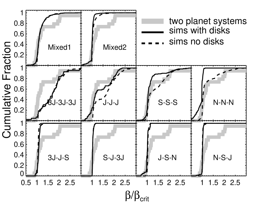
Figure 16.— Cumulative ${\beta/\beta_{crit}}$ distributions for the unstable simulations from each of our ten simulation cases, with (solid lines) and without (dashed lines) planetesimal disks, compared with the observed extra-solar systems exterior to 0.1 AU (thick grey line). Note that one system, HD47186 (Bouchy et al. 2009), has ${\beta/\beta_{crit}}\sim 6$.

Figure 16 compares the cumulative ${\beta/\beta_{crit}}$ distributions for our unstable simulations with the observed two planet extra-solar systems. As seen in Raymondet al. (2009a), ${\beta/\beta_{crit}}$ values from systems with equal-mass planets are far larger than those from systems with planetary mass ratios. This appears to be caused by the vastly larger number of encounters among equal-mass planets before a planet is destroyed.

For the simulations with the most realistic mass distributions (i.e. the Mixed1 and Mixed2 cases) the effect of disks on the $\beta/\beta_{\rm crit}$ is small. Disks do not alter the prediction that scattering yields packed systems. Where there are differences they are in a surprising direction – after an instability systems with planetesimal disks remain closer to the stability boundary (i.e., have lower ${\beta/\beta_{crit}}$ values) than systems with no planetesimal disks. Since planetesimal disks damp eccentricities, they appear to leave the surviving planets in more dynamically compact configurations. This is true even for the low-mass systems such as N-N-N, for which planetesimal scattering almost always induces the migration of one planet out into disk. However, although the outer planet often migrates outward in N-N-N-type cases, the orbits of the inner planets are often compressed by scattering planetesimals outward. So, if we just consider the inner two planets in any system, they appear to end up closer together in the cases with planetesimal disks.

Table 3$p$ values from K-S tests of observations vs. scattering simulations^⋆

	No Disks			With Disks
Set	$p$	$p$	$p$	$p$	$p$	$p$
	(tot)	$({\beta/\beta_{crit}}\leq 1)$	$({\beta/\beta_{crit}}>1)$	(tot)	$({\beta/\beta_{crit}}\leq 1)$	$({\beta/\beta_{crit}}>1)$
Mixed1	0.175	0.005	0.074	0.226	0.818	0.091
Mixed2	0.015	—	0.005	—	0.005	—
3J-3J-3J	—	—	0.016	—	0.012	0.010
J-J-J	0.015	0.012	0.195	0.470	0.111	0.378
S-S-S	0.292	0.425	0.936	0.476	0.328	0.215
N-N-N	0.439	0.438	0.284	—	0.089	—
3J-J-S	—	—	—	0.002	0.313	—
S-J-3J	—	0.012	—	—	1.000	—
J-S-N	—	0.007	—	—	0.008	—
N-S-J	—	—	—	—	0.183	—

^⋆The majority of $p$ values of ’—’ indicate $p<10^{-3}$, and in a few cases insufficient data (e.g., none of the 3J-3J-3J simulations had ${\beta/\beta_{crit}}\leq 1$).

Without disks, the Mixed1, S-S-S and N-N-N simulations all provide good fits to the ${\beta/\beta_{crit}}$ distribution – Table 3 contains $p$ values from K-S tests for each case. However, none of the sets provides a good match for ${\beta/\beta_{crit}}\leq 1$: the S-S-S and N-N-N cases are contaminated by systems which are themselves unstable on timescales longer than our 100 Myr integration time (these were removed by hand in Raymond et al. 2009a but not here). With disks, the S-S-S simulations provide the best match to the known systems and the Mixed1 and J-J-J simulations also provide good fits. In addition, several sets match the distribution very well for ${\beta/\beta_{crit}}\leq 1$ with disks while they failed without disks. The cause of this increase in low-${\beta/\beta_{crit}}$ systems is the presence of mean motion resonances. Systems in resonance tend to have ${\beta/\beta_{crit}}<1$ (Barnes & Greenberg 2007), and these are preferentially set up in systems with planet masses comparable to $M_{\rm J}$ such as the Mixed1 and J-J-J simulations (see §4 below).

4. Mean Motion Resonances (MMRs)

A significant fraction of the known exoplanet systems are thought to lie in mean motion resonances (henceforth MMRs). Marcy et al. (2008), for example, quote a resonant fraction of 18% (4 out of 22 systems). These numbers are currently uncertain because confirmation that systems near resonance are actually librating is often hard to obtain – indeed apparently resonant systems are sometimes revised to be non-resonant (e.g., Fischer et al. 2008). The most likely origin of resonant planets at small orbital radii is convergent migration in gaseous protoplanetary disks (Snellgrove et al. 2001; Lee & Peale 2002; Kley et al. 2004). If this identification is correct, it places bounds on the strength of turbulence within the disk, since even rather modest fluctuations in the disk surface density should destroy resonant alignment (Adams et al. 2008; Lecoanet et al. 2009). Here, we investigate gas free routes to the establishment of resonance due to either pure planet-planet scattering or scattering augmented by the dynamical effect of planetesimals. These channels might contribute to the population of resonance systems at small radii, and potentially dominate it further out where the effects of planetesimal disks are strong.

In previous work related to planet-planet scattering, we studied two mechanisms that can lead to MMRs. First, scattering in isolation (without disks) populates a variety of resonances including high-order MMRs (up to 11th order in our simulations; Raymond et al. 2008a). Second, the planetesimal disk can effectively act as a damping force on planets’ orbits to induce planetary orbits to align into MMRs and sometimes MMR chains (e.g., 4:2:1) with a high efficiency (Raymond et al. 2009b). In this section we study MMRs that arose in both our unstable simulations (via scattering) and our stable simulations (via planet-planetesimal effects). We first introduce the theory of MMRs in §4.1, then examine resonances in unstable (§4.2) and stable (§4.3) systems.

4.1. Definition of Mean Motion Resonances

For mean motion resonance $p+q:p$, resonant arguments $\theta_{i}$ (also called “resonant angles”) are of the form

$$\theta_{1,2}=(p+q)\lambda_{1}-p\lambda_{2}-q\varpi_{1,2}\\$$ (12)

where $\lambda$ are mean longitudes, $\varpi$ are longitudes of pericenter, and subscripts 1 and 2 refer to the inner and outer planet, respectively (e.g., Murray & Dermott 2000). Resonant arguments measure the angle between the two planets at the conjunction point – if any argument librates rather than circulates, then the planets are in resonance. In fact, the bulk of resonant configurations are characterized by only one librating resonant argument (Michtchenko et al. 2008). Frequently, libration occurs around equilibrium angles of zero or 180^∘, but any angle can serve as the equilibrium. Different resonances have different numbers of resonant arguments, involving various permutations of the final terms in Eq. 12. The order of a resonance is given simply by $q$. For example, the 3:1 MMR ($q=2,p=1$) is a second-order resonance that has three resonant arguments:

$$\theta_{1} = 3\lambda_{1}-\lambda_{2}-2\varpi_{1},\hskip 14.45377pt$$

$$\theta_{2} = 3\lambda_{1}-\lambda_{2}-2\varpi_{2},\hskip 7.22743pt{\rm and}\hskip 14.45377pt$$

$$\theta_{3} = 3\lambda_{1}-\lambda_{2}-(\varpi_{1}+\varpi_{2}).$$ (13)

In Raymond et al. (2008a), we found MMRs by targeting systems close to commensurabilities, then looking at individual resonant angles. In this paper we take an automated approach. We devised a simple analysis script to analyze each of our simulations (with and without disks) and calculate all resonant angles for MMRs of up to fourth order. This includes the 2:1, 3:2, 3:1, 5:3, 5:2, and 4:1 MMRs. The script then determined which resonant angles were librating during the last 50 Myr of each simulation. This script is simple and reliable, but it misses the small fraction of cases that enter resonance between 50 and 100 Myr because it requires $\theta$ values to librate for the full interval (50-100 Myr). We impose a cutoff on the libration amplitude $A$ of $A\leq 150^{\circ}$ to avoid false positives, which eliminates some additional systems that are just barely resonant.

4.2. MMRs in unstable systems

In previous work, we found that a few to ten percent of unstable systems could end in MMRs (Raymond et al. 2008a). The resonant fraction depends on the initial planetary mass distribution: MMRs were much more common in systems with radial mass gradients than in simulations that started with equal-mass planets. MMRs are populated by scattering simply because the density of resonant orbits is non-zero. In other words, the last close encounter leading to the destruction of one planet deposits the surviving planets onto orbits which have a chance of being resonant. This mechanism can populate high-order MMRs that are not populated by convergent migration in gaseous disks (Snellgrove et al. 2001; Lee & Peale 2002). The libration amplitudes of resonances populated by scattering are large, which also contrasts with the convergent migration scenario. Thus, as the population of resonant exoplanet systems increases, we may be able to differentiate MMRs caused by scattering vs. convergent migration.

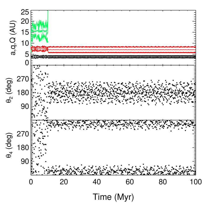
Figure 17.— A 5:2 mean motion resonance set up by scattering. The top panel shows the evolution of the three planets’ semimajor axes $a$, perihelion distances $q$ and aphelion distances $Q$. The middle and bottom panel show two resonant angles for the 5:2 MMR: $\theta_{2}=5\,\lambda_{1}-2\,\lambda_{2}-3\,\varpi_{2}$, and $\theta_{4}=5\,\lambda_{1}-2\,\lambda_{2}-2\,\varpi_{2}-\varpi_{1}$.

Figure 17 shows an example of an MMR caused by planet-planet scattering in a simulation that included a planetesimal disk. After 30,000 years, a close encounter with the outer (1.8 $M_{\rm J}$) planet threw the lower-mass (0.4 $M_{\rm J}$) planet outward into the planetesimal disk, where it remained on a stable but chaotic orbit for about 10 Myr. A final close encounter caused the lower-mass planet to be ejected and placed the surviving (1.9 and 1.8 $M_{\rm J}$) planets in 5:2 MMR. In fact, the two surviving planets are in a special type of resonance called an apsidal corotation resonance in which all resonant angles librate and so does the apsidal alignment (Beaugé et al. 2003). This simulation was unusual because the entire planetesimal disk had been destroyed by the outer planet by the time of the last planetary scattering event such that the behavior was similar to simulations without disks.

Most MMRs that occur in unstable systems with disks arise via a different mechanism. Usually, an instability occurs early in the simulation, removing one planet and placing the two surviving massive ($M_{p}\sim M_{\rm J}$) planets close to resonance. Subsequent interactions with the planetesimal disk act as a damping force that aligns the planetary orbits into MMR. In these cases the outer surviving planet is massive enough to eject most of the planetesimals that it encounters, leading to some inward migration and a compression of the system. In fact, this mechanism has more in common with the generation of MMRs and MMR chains via planetesimal disk interactions (see §4.3 below) than MMRs from pure N-body scattering.

Table 4Mean Motion Resonances in Scattered Systems^⋆

	No Disks			With Disks
Set	1st Order	2nd Order	3rd Order	1st Order	2nd Order	3rd Order
	(frac)	(frac)	(frac)	(frac)	(frac)	(frac)
Mixed1	10 (0.018)	9 (0.016)	3 (0.005)	5 (0.011)	2 (0.005)	1 (0.002)
Mixed2	25 (0.034)	13 (0.017)	8 (0.011)	9 (0.017)	2 (0.004)	1 (0.002)
3J-3J-3J	3 (0.012)	2 (0.008)	0 (—)	0 (—)	0 (—)	0 (—)
J-J-J	1 (0.004)	0 (—)	2 (0.009)	0 (—)	0 (—)	0 (—)
S-S-S	8 (0.022)	3 (0.008)	4 (0.011)	1 (0.005)	1 (0.005)	0 (—)
N-N-N	10 (0.028)	4 (0.011)	4 (0.011)	0 (—)	0 (—)	0 (—)
3J-J-S	1 (0.007)	1 (0.007)	2 (0.013)	1 (0.018)	0 (—)	0 (—)
S-J-3J	1 (0.005)	13 (0.059)	2 (0.009)	0 (—)	6 (0.041)	2 (0.014)
J-S-N	2 (0.010)	4 (0.019)	4 (0.019)	0 (—)	0 (—)	0 (—)
N-S-J	16 (0.072)	4 (0.018)	3 (0.014)	8 (0.054)	1 (0.007)	0 (—)

^⋆The resonance order is given by $q$ in Eqn 12. The first-order MMRs are 2:1 and 3:2, second-order are 3:1 and 5:3, and third-order are 4:1 and 5:2. The values in parentheses represent the fraction of unstable simulations that ended up in each set of MMRs.

The frequency of MMRs from scattering is greatly reduced by the presence of the planetesimal disk (Table LABEL:tab:mmr-scat). In fact, only a small fraction of the MMRs with disks from Table LABEL:tab:mmr-scat are even due to pure scattering – the majority are caused by disk damping as described above. The reason for the absence of MMRs in unstable systems with planetesimal disks is that the low-order MMRs populated by scattering occur preferentially in systems with high mass ratios (for example, almost 10% of the unstable N-S-J simulations yielded 2:1 MMRs), meaning that one planet in the system was relatively low-mass (usually $\sim M_{\rm S}$) and subject to radial migration by planetesimal scattering after the instability placed the planets in resonance.

Thus, scattering appears to be a viable mechanism to populate resonances but its efficiency is reduced in regions which are strongly affected by planetesimal disks. Given that the observed exoplanets do not yet show an obvious signature of planetesimal scattering (see §5 below), some of the known systems could indeed have been populated by this mechanism (Raymond et al. 2008a). However, as we show below, interactions with planetesimal disks in systems that do not experience close encounters and scattering events are vastly more efficient at generating resonant systems.

4.3. MMRs in stable systems

We now consider the generation of MMRs in stable systems that do not experience close encounters between the planets. An empirical argument can be made that such systems are rare amongst the progenitors of currently observed systems, since the good agreement with the observed eccentricity distribution requires that a large fraction of systems are unstable. At larger radii, however, stable systems could be present and perhaps common. In stable systems with relatively massive planets ($M_{p}\gtrsim M_{\rm J}$), the planetesimal disk can act as a damping force and induce planets to align into MMRs. This mechanism is not efficient for low-mass planets because the planetesimal disk has enough angular momentum to cause excessive radial migration and drive the planets apart. However, gentle migration for $M_{p}\sim M_{\rm J}$ is very effective at forming resonant chains reminiscent of the Galilean satellites of Jupiter (Paper 1).

Figure 18.— Example of a 4:2:1 resonant chain in a system of three planets plus an exterior planetesimal disk. Shown are the resonant angles $\theta_{1}=2\,\lambda_{1}-\lambda_{2}-\varpi_{1}$ and $\theta_{2}=2\,\lambda_{1}-\lambda_{2}-\varpi_{2}$ for the inner (left) and outer (right) pairs of planets over the 100 Myr evolution of the simulations. The left panel shows the system including the planetesimal disk, and the right panel has the planets on identical starting orbits but without the planetesimal disk. The simulation is drawn from the Mixed1 set, and the planetary masses are, in increasing orbital distance, 0.98, 1.42, and 1.26 $M_{\rm J}$.

Figure 18 (left panel) shows one example of a 4:2:1 resonant chain for a Mixed1 simulation with three $\sim$ Jupiter-mass planets. The $\theta_{1}$ resonant argument is librating with a small amplitude for both the inner and outer pairs of planets, and for the inner pair $\theta_{2}$ begins to librate after $\sim$ 20 Myr and its libration amplitude decreases over the next 10-20 Myr. The damping effect of the planetesimals is clearly seen as the system moves deeper into the resonance with time, i.e., the libration amplitude of the two resonant arguments decreases. The right panel of Fig. 18 shows the same system with no planetesimal disk. It is clear that this system started with both pairs of planets close to the 2:1 MMR (see Fig. 2) but without the disk the planets do not evolve into the resonance.

Table 5 shows the number of resonances and resonant chains that were set up in each set of stable simulations with planetesimal disks, and that number as a fraction of the total number of stable simulations. For systems with planet masses $M_{\rm S}\lesssim M_{p}\lesssim 3M_{\rm J}$, between roughly 50 and 75 percent of all stable systems ended up with at least one MMR! In addition, up to forty percent of systems were in resonant chains involving all three planets. Recall that our definition of resonance requires at least one resonant argument to librate with an amplitude $A\leq 150^{\circ}$. The second row for each set of simulations shows the number and fraction of systems that were deep in resonance, with $A\leq 60^{\circ}$. Roughly half of the MMRs were deep in resonance, independent of their configuration in the system: both pairs of resonant planets were deep in resonance for about one quarter of the resonant chains.

The vast majority of resonant systems are in the 2:1 MMR, although for lower masses the 3:2 MMR is also common. This is simply because of the location of strong resonances in initial planetary separations vs. mass (Fig. 2). More [less] massive planets start closer to the 2:1 [3:2] MMR, and so given the limited amount of radial migration, tend to end up in that same resonance. The second order MMRs were comprised almost exclusively of the 5:3 MMRs, although those were much rarer than first order MMRs. Depending on the case, about half or slightly less of the resonances were deep, meaning that the libration amplitude was $60^{\circ}$ or less. Systems that were extremely deep in the resonance, however, were rare: indeed only a single case with $A<10^{\circ}$ was found in the entire ensemble of simulations. This is of interest since dynamical modeling of the GJ 876 system shows that one of the resonant angles librates with an amplitude that is, at most, $\theta=7^{\circ}\pm 2^{\circ}$ (Laughlin et al. 2005). Taken at face value, one concludes that capture into resonance due to gas disk migration is not only the favored explanation for the origin of the GJ 876 system itself, but that gas rather than planetesimal effects would also be needed to explain hypothetical analogs of GJ 876 that might be discovered very deep in resonance at large orbital radii. We caution, however, that we have not demonstrated that the distribution of libration amplitudes is independent of numerical details of our simulations, and in particular that it is independent of the mass of particles used to represent the disk. Further simulations would be needed to study the predicted distribution of $A$ in more detail.

Figure 19.— Semimajor axis shifts (i.e., final minus starting values) for the planets in the stable Mixed1 and Mixed2 systems. Positive shift values indicate a convergence of the two planets and negative values indicate a divergence; i.e., positive $y$ axis values indicate that the middle and outer planets converged over the course of the simulation, and positive $x$ axis values mean that the inner and middle planets converged. Filled circles are systems that contain at least one pair of resonant planets, and open circles are nonresonant systems.

What causes the resonances in these systems? Figure 19 shows the semimajor axis shifts of the planets in the stable Mixed1 and Mixed2 systems: positive values indicate convergence and negative indicate divergence. There is a much more limited range of parameter space for convergence than divergence, since for massive planets the stability limit is located in the vicinity of the 3:2 MMR. Planet pairs were limited to converging $\lesssim 0.1$ AU, but divergence was unlimited, at least for the outer pair of planets (too much divergence of the inner pair could impinge on the outer planet).

Table 5 shows that MMRs generally occur at a higher frequency in systems that converge rather than diverge. However, for most giant planet configurations, systems for which all three planets converge are rare. The exception are the systems with positive mass gradients (S-J-3J and N-S-J), for which almost half the stable systems converged. This is because they contain a very massive outer planet capable of quickly ejecting planetesimals rather than scattering them inward, thereby migrating slightly inward. In contrast, systems with negative mass gradients (3J-J-S and J-S-N) favor divergence because the innermost planet is the ejector and the outer two preferentially scatter planetesimals inward and migrate outward. For massive equal-mass planets (J-J-J and 3J-3J-3J), it is often the case that the inner two planets converge while the outer two diverge. This is caused simply by the outer planet scattering planetesimals in to the middle planet. With higher relative velocities the middle planet can more easily eject the planetesimals, causing it to migrate inward, away from the outer planet but toward the inner one.

Table 5Mean Motion Resonances and Resonant Chains in Stable Systems^⋆

Set	MMRs (frac)	2:1	3:2	2nd order	MMR chains	4:2:1 chains
	deep	deep	deep	deep	deep	deep
Mixed1	379 (0.706)	335 (0.624)	58 (0.108)	20 (0.037)	197 (0.367)	157 (0.292)
	190 (0.354)	174 (0.324)	12 (0.022)	7 (0.013)	50 (0.093)	47 (0.088)
Mixed2	162 (0.348)	127 (0.273)	47 (0.101)	13 (0.028)	54 (0.116)	28 (0.060)
	77 (0.166)	61 (0.131)	16 (0.034)	5 (0.011)	13 (0.028)	6 (0.013)
3J-3J-3J	351 (0.708)	351 (0.708)	0 (—)	0 (—)	60 (0.121)	59 (0.119)
	122 (0.246)	122 (0.246)	0 (—)	0 (—)	3 (0.006)	3 (0.006)
J-J-J	217 (0.764)	213 (0.750)	0 (—)	6 (0.021)	114 (0.401)	113 (0.398)
	103 (0.363)	101 (0.356)	0 (—)	2 (0.007)	18 (0.063)	18 (0.063)
S-S-S	61 (0.477)	3 (0.023)	60 (0.469)	1 (0.008)	15 (0.117)	0 (—)
	22 (0.172)	2 (0.016)	22 (0.172)	1 (0.008)	1 (0.008)	0 (—)
N-N-N	0 (—)	0 (—)	0 (—)	0 (—)	0 (—)	0 (—)
	0 (—)	0 (—)	0 (—)	0 (—)	0 (—)	0 (—)
3J-J-S	92 (0.571)	92 (0.571)	1 (0.006)	0 (—)	1 (0.006)	0 (—)
	73 (0.453)	73 (0.453)	0 (—)	0 (—)	0 (—)	0 (—)
S-J-3J	76 (0.927)	76 (0.927)	21 (0.256)	11 (0.134)	37 (0.451)	5 (0.061)
	63 (0.768)	63 (0.768)	4 (0.049)	3 (0.037)	7 (0.085)	0 (—)
J-S-N	24 (0.118)	24 (0.118)	0 (—)	0 (—)	0 (—)	0 (—)
	12 (0.059)	12 (0.059)	0 (—)	0 (—)	0 (—)	0 (—)
N-S-J	23 (0.793)	11 (0.379)	13 (0.448)	11 (0.379)	7 (0.241)	0 (—)
	8 (0.276)	2 (0.069)	6 (0.207)	5 (0.172)	3 (0.103)	0 (—)

^⋆Each column is the number, and in parentheses the fraction, of a systems in a given resonance that occurred for each set of stable simulations. Resonances are defined to exhibit libration of at least one resonant argument with libration angle $A<150^{\circ}$. For each set of simulations, the second row represents the same resonance but requiring that the system be deep in the resonance, with $A<60^{\circ}$.

Among the simulations with radial mass gradients, MMRs are more common in systems with a more massive outer planet (those with positive mass gradients, S-J-3J and N-S-J). This is because the massive outer planet confines the planetary system, and the planetesimal scattering causes the system to converge, as a whole or for one pair of planets, much more frequently than for a lower-mass outer planet. Indeed, the frequency of MMRs as a whole correlates with the fraction of systems which converge rather than diverge (see Tables 5 and 6). Nonetheless, many MMRs are created in divergent systems, simply because planets were initially placed near strong MMRs (Fig. 2).

Table 6Sources of MMRs in Stable Systems^⋆

Set	MMRs	conv-conv	conv-div	div-conv	div-div
		(frac)	(frac)	(frac)	(frac)
Mixed1	392	0.11 (0.86)	0.24 (0.79)	0.24 (0.77)	0.41 (0.58)
Mixed2	184	0.05 (0.90)	0.05 (0.78)	0.27 (0.58)	0.63 (0.16)
3J-3J-3J	351	0.23 (0.65)	0.35 (0.73)	0.24 (0.69)	0.18 (0.75)
J-J-J	218	0.29 (0.78)	0.38 (0.75)	0.22 (0.75)	0.10 (0.79)
S-S-S	65	0.00 (—)	0.07 (1.00)	0.19 (0.67)	0.73 (0.34)
N-N-N	0	0.00 (—)	0.00 (—)	0.00 (—)	1.00 (0.00)
3J-J-S	93	0.00 (—)	0.07 (0.92)	0.13 (0.71)	0.80 (0.52)
S-J-3J	84	0.43 (0.97)	0.33 (0.81)	0.22 (1.00)	0.02 (1.00)
J-S-N	24	0.00 (—)	0.00 (—)	0.00 (—)	1.00 (0.12)
N-S-J	39	0.45 (0.62)	0.38 (0.82)	0.10 (0.67)	0.07 (1.000)

^⋆Each column containing ’conv’ or ’div’ denotes the fraction of stable simulations in which the planets are either converging or diverging. The first ’conv’/’div’ refers to the inner pair of planets and the second to the outer pair. The fraction in parentheses denotes the fraction of those cases which ended up with at least one pair of resonant planets.

5. Models for the observed distributions of extrasolar planets

In this Section we investigate quantitatively whether the observed distributions of extrasolar planets can be reproduced from our scattering simulations. We focus primarily on the eccentricity distribution, since this is the most accurately measured statistical property of extrasolar planetary systems. At the outset we observe that we are not claiming that our model can explain both the radial distribution and eccentricity of observed planets. Roughly half of the observed planets orbit at radii less than 1 AU, which is a region of semi-major axis space that is not heavily populated by our simulations (Fig. 15). Our systems do, however, overlap with those planets known at radii of a few AU, and these planets appear to share roughly the same eccentricity distribution as planets at smaller radii (Rasio & Ford 2008).

5.1. The problem of the mass-eccentricity correlation

For the Mixed1 simulations we generated planet masses by sampling the observed planetary mass function randomly and independently, using mass limits of $M_{\rm Sat}<M<3\ M_{\rm J}$. Since the eccentricity distribution that results from these initial conditions matches the data closely (Fig. 6) – irrespective of whether we include disks or not – it might appear as if there is no further problem to solve. This ignores the fact that the observed exoplanet eccentricity distribution is also mass-dependent: lower-mass planets have lower eccentricities than higher-mass planets (Ribas & Miralda-Escudé 2007; Ford & Rasio 2008; Wright et al. 2009). The evidence for this correlation appears to be strong. If we divide the sample of known extra-solar planets into low-mass ($M_{p}\sin i<M_{\rm J}$) and high-mass ($M_{p}\sin i>M_{\rm J}$) bins, we find a Kolmogorov-Smirnov probability $p$ of only 0.002 that they are drawn from the same distribution.

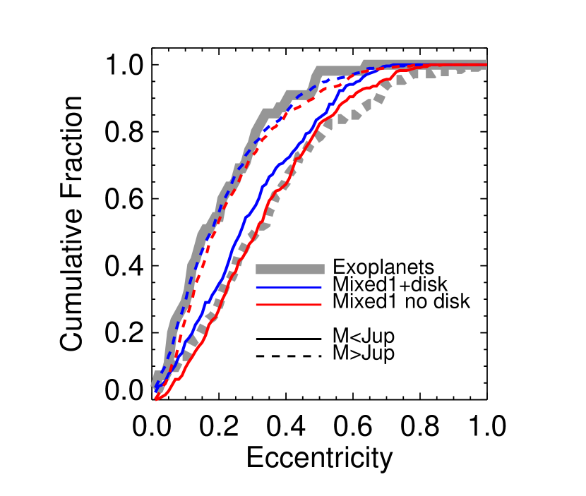
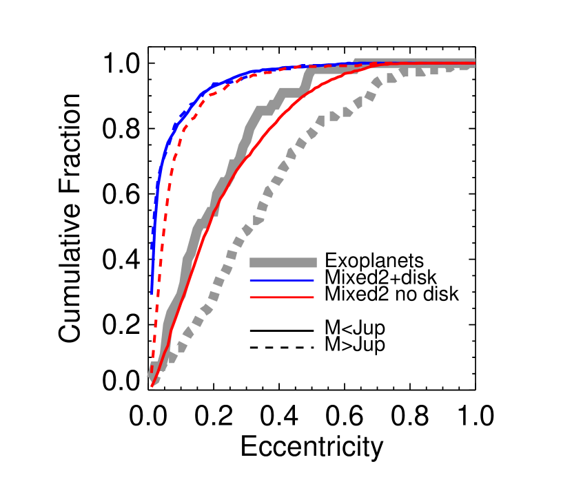
Figure 20.— Cumulative eccentricity distributions for the unstable Mixed1 (left panel) and Mixed2 (right panel), with (blue lines) and without (red lines) disks, compared with the observed extra-solar planets beyond 0.l AU (thick grey lines). Each group was divided by the planet mass: $M_{p}<M_{\rm J}$ are the solid lines and $M_{p}>M_{\rm J}$ are dashed lines.

Assuming that this trend is real we have a clear problem: scattering does not predict that low-mass planets should be less eccentric than high-mass ones. Figure 20 shows eccentricity distributions for the Mixed1 and Mixed2 simulations divided into the same low-mass ($M_{p}<M_{\rm J}$) and high-mass categories for cases with and without disks. The predicted trend is opposite to that observed. Indeed, once the sample has been split into mass bins it becomes clear that the good agreement of the overall distribution is somewhat fortuitous. It occurs because – for the Mixed1 simulations – the low-mass simulations match the observed high-mass curve and vice-versa! Changing the lower mass limit for the mass function sampling to $10\ M_{\oplus}$ only makes matters worse. For the simulations with no disks, the more massive planets are even less eccentric than for the Mixed1 simulations simply because the typical mass ratio in a given scattering event is larger for the Mixed2 simulations. It is interesting to note that for the Mixed2 simulations with disks the high- and low-mass planets have virtually identical eccentricity distributions, meaning that the tendency for low-mass planets to acquire large eccentricities during scattering is almost exactly balanced by the eccentricity damping of the disk.

5.2. A solution from planet mass correlations

The above problem raises a simple question, is it possible to simultaneously match the observed constraints on,

• The total eccentricity distribution,

• The mass-eccentricity correlation, and

• The mass function,

using a scattering model? Although our data are not able to provide a rigorous answer we contend that solutions are possible, either with or without appealing to the existence of planetesimal disks. In the absence of disks, the key assumption that we must drop is that planet masses in the same system are chosen independently from the overall mass function. If, instead, we allow for correlations between planet masses, the extra degree of freedom allows us to match what is seen observationally.

For a disk-free solution, we start with the equal-mass simulations and choose a weighted combination of the 3J-3J-3J, J-J-J, and S-S-S simulations that matches the observed mass distribution (i.e., that contains correspondingly more low-mass than high-mass systems). By construction this matches the mass distribution, and does a reasonable job at matching the total eccentricity distribution (the K-S $p$ value is 0.09). However, this combination does not match the mass-eccentricity distribution; both the high-mass and low-mass planets have large eccentricities, and in fact, both provide a match to the $M_{p}>M_{\rm J}$ exoplanets. The high-mass planets have slightly higher eccentricities than the low-mass planets (see Fig. 6) but the difference is small because the highest-eccentricity systems (3J-3J-3J) are very weakly-weighted to match the observed mass distribution. Note that we count Jupiter-mass planets in both the high-mass and low-mass bins.

We now mix in systems for which low-mass planets have lower eccentricities than high-mass planets. In the absence of disks, this can be done if we assume that high-mass and low-mass planetary systems are fundamentally different. Specifically, we assume that high-mass systems form roughly equal-mass planets yielding large eccentricities, whereas low-mass systems form a much wider variety of systems and tend to have lower eccentricities. To show that this works, at least approximately, we assume that the J-S-N and N-S-J simulations yield an eccentricity distribution that is representative of the scattering among unequal-mass low-mass planets (with masses up to, but not beyond, $M_{\rm J}$). We then add J-S-N and N-S-J simulations to the total and low-mass eccentricity distributions, but not to the high-mass distribution. We gave the J-S-N/N-S-J systems the same abundance as the S-S-S systems such that the low-mass systems are equally divided between equal-and unequal-mass cases (except for a small contribution from the J-J-J simulations).

The upshot of this cookery is shown in Figure 21. The blended distribution, which is roughly consistent with the mass function, provides a decent match to both the total eccentricity distribution and to the mass-eccentricity distributions. The K-S test $p$ values are 0.25 (for the total distribution), 0.09 (for the low-mass planets) and 0.20 (for the high-mass planets). It is evident that matching the low mass planets is by no means easy, and in fact our “solution” is close to being statistically unacceptable. Nonetheless, it is clearly possible to reverse the natural tendency of scattering to generate larger $e$ for low-mass planets by strongly correlating the masses of planets. We further believe – though we do not have the data to demonstrate it – that the magnitude of the observed mass-eccentricity correlation lies within the range that could be accurately reproduced by fine tuning the mix of initial conditions used.

5.3. A solution from disk damping

An entirely different solution to the mass-eccentricity problem invokes the damping effects of planetesimal disks. Disks referentially damp the eccentricities of the smallest planets (Fig. 8), but, as we have noted, the effect correlates most strongly with the total system mass rather than that of individual planets. We therefore consider the equal-mass cases, and (as before) blend the 3J-3J-3J, J-J-J, and S-S-S simulations such as to approximate a three-bin version of the mass function. We assume that a fraction $F=1/2$ of the systems are affected by disks, while the rest are not. This combination provides reasonable matches for both the total eccentricity distribution ($p$ = 0.08) as well as the low-mass ($p$ = 0.02) and high-mass ($p$ = 0.44) planets (red curves in Fig. 21). The match for the low-mass planets can be improved by slightly increasing $F$, at the expense of the fit to the overall distribution.

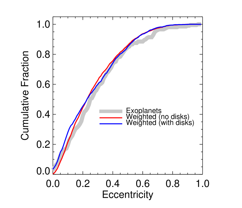
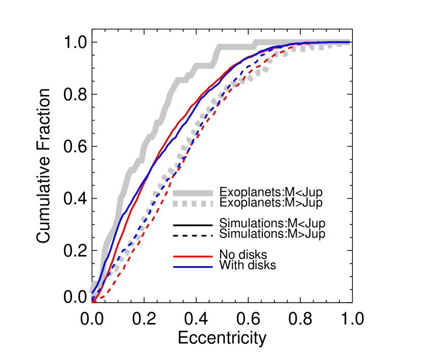
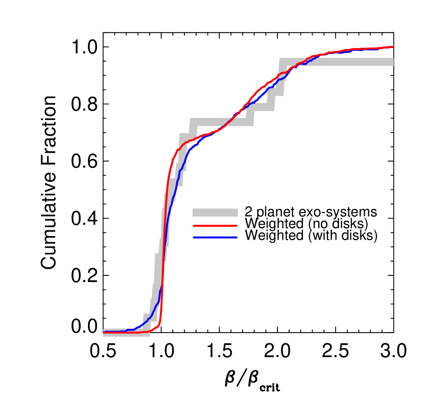
Figure 21.— Comparison between our two weighted combinations of initial conditions with the observed distributions. The left panel shows the total cumulative eccentricity distribution, and center panel shows the mass-eccentricity distribution: $M_{p}<M_{\rm J}$ are the solid lines and $M_{p}>M_{\rm J}$ are dashed lines. We have only included observed planets beyond 0.l AU (thick grey lines). The right panel shows the distributions compared with the observed ${\beta/\beta_{crit}}$ values of known two planet systems.

Do the two weighted distributions match other observations? Using the same combination of different sets of simulations we generated weighted distributions of ${\beta/\beta_{crit}}$ to compare with observations, seen in the third panel of Fig. 21. Remarkably, both combinations of simulations provide excellent fits to the distribution of separations in two planet systems. The weighted case with disks was a better fit to the ${\beta/\beta_{crit}}$ distribution (K-S $p$ values of 0.20 with no disks and 0.72 with disks), largely because the cases with disks were able to fit the distribution of values at ${\beta/\beta_{crit}}\leq 1$ which are dominated by resonant systems. Thus, the ${\beta/\beta_{crit}}$ distribution cannot differentiate between the two weighted combinations of simulations we have constructed. However, it is interesting that both weighted distributions can match all of the currently well-observed constraints.

5.4. Discussion

What can we conclude from this proof-of-principle exercise? First, correlations between planet masses in the same system can qualitatively alter some of the predictions of scattering models. Although we have here allowed ourselves complete freedom to impose whatever correlations we need, our disk-free solution in fact involves physically conceivable variations in the outcome of planet formation in different disks. A massive disk of gas and solids would be expected to form several cores that go on to accrete substantial envelopes, such that the outcome is usually a system with several very massive planets. A less massive disk, on the other hand, may only form one relatively low mass gas giant together with a number of low mass core-dominated planets. Second, the effects of planet-planet scattering with mass correlations, and the effects of planetesimals, can be almost indistinguishable, at least for the distributions we have considered. This should be borne in mind, especially as observations probe larger orbital radii where it is more probable that planetesimal disks play a dynamical role.

Notwithstanding the formal degeneracy of our solutions, the disk-free solution is favored as the origin of currently observed eccentricities. The reason is simply that the current sample includes many planets at radii that are simply too small to have experienced damping from plausible planetesimal disks (note that our inner disk radius of 10 AU is already smaller than is often assumed). The match is not perfect but this is not surprising, since the comparison is not entirely fair. Both the observed and predicted eccentricities depend upon the Safronov number, defined as the ratio of the escape speed from a planet’s surface to the escape speed from the planetary system at that location,

$$\Theta^{2}=\left(\frac{M_{p}}{M_{\star}}\right)\left(\frac{a}{R}\right),$$ (14)

where $M_{p}$ and $M_{\star}$ are the planetary and stellar mass, $a$ is the orbital distance and $R$ is the planetary radius (Ford & Rasio 2008). Our simulations probe the region at somewhat larger $a$ than is currently observed, such that the $\Theta$ values are correspondingly higher. Only at higher planetary masses are the $\Theta$ values large enough that the variations in $\Theta$ between our simulations and the observed planets are too small to affect the eccentricities, and it is reassuring that our weighted fits match the high-mass planets quite well. Another point to bear in mind is that although the selection function of radial velocity surveys is approximately independent of eccentricity (Cumming et al. 2008), there are almost certainly systematic errors to add to the purely statistical errors that we have used (e.g. Shen & Turner 2008).

We do not expect the degeneracy between disks and mass correlations to persist to arbitrarily large orbital radii. Disk damping becomes increasingly more important as the semi-major axis increases, and as the planet mass decreases. For very low mass planets the resulting reduction in eccentricity is greater than could be explained by any plausible blend of simulations with different conditional mass functions. An ongoing trend to lower eccentricities for low mass planets, as the orbital radius increases, would thus be a strong sign of dynamical influence from planetesimal disks.

6. Discussion and Conclusions

We have presented an extensive study of the dynamics of planetary systems that evolve under the joint action of planet-planet and planetesimal disk scattering. The model is founded on the assumption that giant planets form in marginally stable configurations interior to substantial disks of small bodies that failed to form planets or cores. Persuasive (but circumstantial) observational and theoretical arguments suggest generically similar initial conditions, and physical mechanisms, describe the evolution of typical outer planetary systems subsequent to gas disk dispersal. We have simulated the evolution using a large set of N-body integrations, designed such that the statistical errors on the model predictions remain smaller than the uncertainty in observed data. Achieving this level of fidelity is still relatively easy for models that invoke only planet-planet scattering, but requires substantial investment of computing resources (amounting to several million core hours in our case) once disks are included.

The main conclusions of our study are:

• Dynamical models for the outer Solar System such as the Nice model, in which small body scattering dominates (Tsiganis et al. 2005), and pure planet-planet scattering models for eccentric exoplanets, are limiting cases of a joint model that includes both scattering processes. Future extrasolar planet surveys are likely to uncover systems in which the two processes were of comparable importance.

• The past dynamical effects of planetesimal disks are observable statistically as a trend toward lower eccentricities for low mass planets at larger orbital radius. The strongest trend is predicted to be a correlation between eccentricity and the total mass of surviving planets in the system. The transition radii and masses at which the effects of disks should become apparent are not known. Our specific model predicts clear effects for $\approx 0.5\ M_{\rm J}$ planets at 5-10 AU. Observations in this region of parameter space will provide important constraints on the typical properties (the mass and inner radius) of outer planetesimal disks. Useful constraints would be possible from radial velocity surveys capable of detecting planets with radial velocity amplitudes $K\approx 5\ {\rm m\ s}^{-1}$ and periods in excess of 10 years.

• Planetary inclination with respect to the initial orbital plane, and the mutual inclination in multiple planet systems, is damped by disks in the same way as is eccentricity. Our initial conditions (with the number of planets fixed at $N=3$) can yield significant inclinations when disks are unimportant ($30^{\circ}$ is not uncommon), but do not form polar or retrograde systems.

• Planet-planet scattering can reproduce the eccentricity distribution of known extrasolar planets (Chatterjee et al. 2008; Jurić & Tremaine 2008), given only the additional assumption that the initial conditions were unstable to close planetary encounters (this is a subset of our initial conditions). Planetesimal disks do not destroy this agreement for planet masses and orbital radii characteristic of the currently observed sample.

• The observed variation of the eccentricity distribution with planet mass (Ford & Rasio 2008; Wright et al. 2009) is in the opposite sense to that predicted by simple planet-planet scattering models. The observed trend can probably be reproduced if we postulate strong correlations between planet masses in the same system. Specifically, we require that one set of systems must preferentially form massive planets of comparable masses, while the rest form lower mass planets with a wider range of masses. This implies that the planetary mass function is a global quantity that does not apply on the level of single systems.

• At radii modestly larger than those currently probed by observations, the effects of planetary mass correlations and planetesimal disks on the eccentricity distribution can be almost identical. Additional constraints are required to break the degeneracy and thereby determine which physical processes are at work.

• Scattering forms dynamically packed planetary systems, in which the final separation of two planet systems clusters close to the Hill stability boundary (Raymond et al. 2009b). The presence of planetesimal disks causes the final systems, on average, to be even more closely packed, at least when only the innermost pair of surviving planets are considered.

• It is probable that the formation of planets at intermediate and large radii (beyond 5 AU) yields an admixture of stable initial conditions (those that do not result in close planetary encounters). Stable systems with $\sim$Jupiter-mass planets should produce an abundance of low-order mean motion resonances. In many cases there should exist resonant chains analogous to the 4:2:1 Laplace resonance among Jupiter’s Galilean satellites. Although the observed orbital arc is short, stability analyses suggest that the HR 8799 system (Marois et al. 2008) may be the first example of such a resonant chain in the exoplanet population (Fabrycky & Murray-Clay 2008; Reidemeister et al. 2009). We expect a large fraction of outer, high-mass giant planets to be discovered to be in resonance, especially if their orbits display the low eccentricities indicative of stable systems.

• The predicted number of high mass planets on highly eccentric orbits with large apocenter distances is unaffected by the presence of planetesimal disks. The number of low mass planets on such orbits is, however, greatly reduced. The existence of the high mass systems is a secure prediction of scattering models (Veras et al. 2009; Scharf & Menou 2009), and provides an attractive target for direct imaging surveys of young stars.

The initial conditions and physical processes modeled in this work are idealized. We have assumed that the properties of the planetesimal disk are universal, so that variations between systems arise solely due to different planetary masses and architectures. To a first approximation this is justifiable. Giant planets can accrete vastly different envelopes – from a few Earth masses in the case of ice giants up to many Jupiter masses at the high end – depending upon when runaway accretion occurs relative to the lifetime of the gas disk (Pollack et al. 1996). The dispersion in giant planet masses is thus plausibly larger than the dispersion in the masses of planetesimal disks. In more detail, however, we expect the masses and radial extent of planetesimal disks to vary between systems, in a manner than is largely unconstrained outside the Solar System (where disk masses of $\approx 30-50\ M_{\oplus}$ are inferred; Tsiganis et al. 2005). A physical dispersion in disk properties would smooth the transition between the planet-planet and planetesimal dominated regimes that we have identified.

We have also assumed that purely N-body dynamics dominates the evolution. Is the neglect of gas disk interactions (including migration, accretion, and damping or excitation of eccentricity) justified? This depends upon how the timescale for dynamical instability compares to the local gas dispersal timescale. Using our initial conditions the onset of dynamical instability typically requires a timescale of the order of $10^{5}$ yr, though there are some systems that become unstable much more rapidly. Both observations (Simon & Prato 1995; Wolk & Walter 1996) and models (Alexander, Clarke & Pringle 2006; Chiang & Murray-Clay 2007) peg the global disk dispersal timescale at $\sim 10^{5}$ yr, and gas is likely to disperse locally from any particular radius substantially more rapidly. Thus, very rapid instabilities probably do occur in the presence of residual gas (Moeckel et al. 2008), but most take place in an almost gas-free environment.

The fact that the neglect of gas is (almost) self-consistent is, of course, a restatement of our initial planetary separations, which were chosen precisely to yield mostly late-onset instability. As we have noted, the relatively widely spaced planets we start with also yield (especially in the presence of disks) stable systems, which have quite different dynamical properties. This causes difficulties if we try to envisage physically motivated initial conditions that can explain the observed properties of extrasolar planets. Matching the eccentricity distribution requires that a large fraction of planets start in unstable configurations, but this can only be achieved for systems that start in configurations slightly more compact than those we have assumed. The neglect of gas may be harder to justify in that case. Similarly, initial conditions that start with several planets on long term unstable orbits are easiest to justify if the planets experienced a period of resonant locking before finally detaching from resonance. However, although there are plausible mechanisms that might first establish and then break a resonant lock (Adams et al. 2008; Lecoanet et al. 2009), it is hard to see why the lock should typically be broken close to the epoch when the gas is dispersed (possibly variations in the strength of turbulence when a weak disk becomes well-ionized may play a role). We have no solutions to these puzzles, but they alert us to the possibility that the typical properties of extrasolar planets at larger orbital radii may be determined largely by a changing mixture of stable and unstable initial conditions. As we have emphasized, the presence of stable initial configurations results in a very high resonant fraction among massive planets, and this is likely to be the most distinctive observational signature that such systems exist.

Finally, we note that parallel (and possibly more powerful) constraints on models of the type we have proposed are available via the study of dust production and debris disks (Wyatt 2008). These aspects can be studied by coupling our dynamical simulations to a collisional evolution model (Booth et al. 2009). We plan to study this, along with the influence of the evolution we have described on hypothetical terrestrial planets, in future papers.

References

- Adams & Laughlin (2003) Adams, F. C., & Laughlin, G. 2003, Icarus, 163, 290
- Adams et al. (2008) Adams, F. C., Laughlin, G., & Bloch, A. M. 2008, ApJ, 683, 1117
- Alexander, Clarke & Pringle (2006) Alexander, R. D., Clarke, C. J., & Pringle, J. E. 2006, MNRAS, 369, 229
- Andrews & Williams (2007) Andrews, S. M., & Williams, J. P. 2007, ApJ, 659, 705
- Armitage (2007) Armitage, P. J. 2007, ApJ, 665, 1381
- Armitage (2010) Armitage, P. J. 2010, Astrophysics of Planet Formation, Cambridge University Press: Cambridge
- Armitage et al. (2002) Armitage, P. J., Livio, M., Lubow, S. H., & Pringle, J. E. 2002, MNRAS, 334, 248
- Asghari et al. (2004) Asghari, N., et al. 2004, A&A, 426, 353
- Barnes et al. (2008) Barnes, R., Goździewski, K., & Raymond, S. N. 2008, ApJ, 680, L57
- Barnes & Greenberg (2007) Barnes, R., & Greenberg, R. 2007, ApJ, 665, L67
- Barnes & Greenberg (2006) Barnes, R., & Greenberg, R. 2006, ApJ, 647, L163
- Barnes & Quinn (2004) Barnes, R., & Quinn, T. 2004, ApJ, 611, 494
- Barnes & Raymond (2004) Barnes, R., & Raymond, S. N. 2004, ApJ, 617, 569
- Bean & Seifahrt (2009) Bean, J. L., & Seifahrt, A. 2009, A&A, 496, 249
- Bean et al. (2008) Bean, J. L., McArthur, B. E., Benedict, G. F., & Armstrong, A. 2008, ApJ, 672, 1202
- Beaugé et al. (2003) Beaugé, C., Ferraz-Mello, S., & Michtchenko, T. A. 2003, ApJ, 593, 1124
- Bodenheimer et al. (2000) Bodenheimer, P., Hubickyj, O., & Lissauer, J. J. 2000, Icarus, 143, 2
- Booth et al. (2009) Booth, M., Wyatt, M. C., Morbidelli, A., Moro-Martin, A., & Levison, H. F. 2009, MNRAS, 399, 385
- Bouchy et al. (2009) Bouchy, F., et al. 2009, A&A, 496, 527
- Butler et al. (2006) Butler, R. P., et al. 2006, ApJ, 646, 505
- Catlett, C. et al. (2007) Catlett, C. et al. 2007, HPC and Grids in Action, Ed. Lucio Grandinetti, IOS Press ’Advances in Parallel Computing’ series, Amsterdam, 2007.
- Chambers (1999) Chambers, J. E. 1999, MNRAS, 304, 793
- Chambers et al. (1996) Chambers, J. E., Wetherill, G. W., & Boss, A. P. 1996, Icarus, 119, 261
- Chatterjee et al. (2008) Chatterjee, S., Ford, E. B., Matsumura, S., & Rasio, F. A. 2008, ApJ, 686, 580
- Chiang et al. (2002) Chiang, E. I., Fischer, D., & Thommes, E. 2002, ApJ, 564, L105
- Chiang & Murray-Clay (2007) Chiang, E., & Murray-Clay, R. 2007, Nature Physics, 3, 604
- Chiang et al. (2003) Chiang, E. I., et al. 2003, AJ, 126, 430
- Cumming et al. (2008) Cumming, A., Butler, R. P., Marcy, G. W., Vogt, S. S., Wright, J. T., Fischer, D. A. 2008, PASP, 120, 531
- D’Angelo et al. (2006) D’Angelo, G., Lubow, S. H., & Bate, M. R. 2006, ApJ, 652, 1698
- Fabrycky & Murray-Clay (2008) Fabrycky, D. C., & Murray-Clay, R. A. 2008, arXiv:0812.0011
- Fabrycky & Winn (2009) Fabrycky, D. C., & Winn, J. N. 2009, ApJ, 696, 1230
- Fernandez & Ip (1984) Fernandez, J. A., & Ip, W.-H. 1984, Icarus, 58, 109
- Fischer et al. (2008) Fischer, D. A., et al. 2008, ApJ, 675, 790
- Ford & Chiang (2007) Ford, E. B., & Chiang, E. I. 2007, ApJ, 661, 602
- Ford et al. (2001) Ford, E, B., Havlickova, M., & Rasio, F. A. 2001, Icarus, 150, 303
- Ford & Rasio (2008) Ford, E. B., & Rasio, F. A. 2008, ApJ, 686, 621
- Ford et al. (2003) Ford, E. B., Rasio, F. A., & Yu, K. 2003, Scientific Frontiers in Research on Extrasolar Planets, 294, 181
- Gaudi & Winn (2007) Gaudi, B. S., & Winn, J. N. 2007, ApJ, 655, 550
- Gladman (1993) Gladman, B. 1993, Icarus, 106, 247
- Goldreich (1965) Goldreich, P. 1965, MNRAS, 130, 159
- Goldreich & Tremaine (1980) Goldreich, P., & Tremaine, S. 1980, ApJ, 241, 425
- Goldreich et al. (2004) Goldreich, P., Lithwick, Y., & Sari, R. 2004, ARA&A, 42, 549
- Goldreich & Sari (2003) Goldreich, P., & Sari, R. 2003, ApJ, 585, 1024
- Gomes et al. (2005) Gomes, R., Levison, H. F., Tsiganis, K., & Morbidelli, A. 2005, Nature, 435, 466
- Gomes et al. (2004) Gomes, R. S., Morbidelli, A., & Levison, H. F. 2004, Icarus, 170, 492
- Hébrard et al. (2008) Hébrard, G., et al. 2008, A&A, 488, 763
- Hahn & Malhotra (2005) Hahn, J. M., & Malhotra, R. 2005, AJ, 130, 2392
- Hahn & Malhotra (1999) Hahn, J. M., & Malhotra, R. 1999, AJ, 117, 3041
- Ida et al. (2000) Ida, S., Bryden, G., Lin, D. N. C., & Tanaka, H. 2000, ApJ, 534, 428
- Jackon et al. (2008) Jackson, B., Greenberg, R., & Barnes, R. 2008, ApJ, 678, 1396
- Jewitt & Luu (1993) Jewitt, D., & Luu, J. 1993, Nature, 362, 730
- Jones et al. (2001) Jones, B. W., Sleep, P. N., & Chambers, J. E. 2001, A&A, 366, 254
- Jurić & Tremaine (2008) Jurić, M., & Tremaine, S. 2008, ApJ, 686, 603
- Kirsh et al. (2009) Kirsh, D. R., Duncan, M., Brasser, R., & Levison, H. F. 2009, Icarus, 199, 197
- Kley et al. (2004) Kley, W., Peitz, J., & Bryden, G. 2004, A&A, 414, 735
- Kopparapu et al. (2009) Kopparapu, R. K., Raymond, S. N., & Barnes, R. 2009, ApJ, 695, L181
- Laskar (1997) Laskar, J. 1997, A&A, 317, L75
- Laughlin et al. (2005) Laughlin, G., Butler, R. P., Fischer, D. A., Marcy, G. W., Vogt, S. S., & Wolf, A. S. 2005, ApJ, 622, 1182
- Lecoanet et al. (2009) Lecoanet, D., Adams, F. C., & Bloch, A. M. 2009, ApJ, 692, 659
- Lee & Peale (2002) Lee, M. H., & Peale, S. J. 2002, ApJ, 567, 596
- Lee & Thommes (2009) Lee, M. H., & Thommes, E. W. 2009, ApJ, 702, 1662
- Levison & Duncan (2000) Levison, H. F., & Duncan, M. J. 2000, AJ, 120, 2117
- Levison & Morbidelli (2003) Levison, H. F., & Morbidelli, A. 2003, Nature, 426, 419
- Levison et al. (2008) Levison, H. F., Morbidelli, A., Vanlaerhoven, C., Gomes, R., & Tsiganis, K. 2008, Icarus, 196, 258
- Lin et al. (1996) Lin, D. N. C., Bodenheimer, P., & Richardson, D. C. 1996, Nature, 380, 606
- Lin & Ida (1997) Lin, D. N. C., & Ida, S. 1997, ApJ, 477, 781
- Lin & Papaloizou (1986) Lin, D. N. C., & Papaloizou, J. 1986, ApJ, 309, 846
- Lubow & Ogilvie (2001) Lubow, S. H., & Ogilvie, G. I. 2001, ApJ, 560, 997
- Malhotra (1995) Malhotra, R. 1995, AJ, 110, 420
- Malhotra (1993) Malhotra, R. 1993, Nature, 365, 819
- Marchal & Bozis (1982) Marchal, C., & Bozis, G. 1982, Celestial Mechanics, 26, 311
- Marcy et al. (2008) Marcy, G. W., et al. 2008, Physica Scripta Volume T, 130, 014001
- Marcy et al. (2001) Marcy, G. W., Butler, R. P., Fischer, D., Vogt, S. S., Lissauer, J. J., & Rivera, E. J. 2001, ApJ, 556, 296
- Marcy et al. (2005) Marcy, G. W., Butler, R. P., Vogt, S. S., Fischer, D. A., Henry, G. W., Laughlin, G., Wright, J. T., & Johnson, J. A. 2005, ApJ, 619, 570
- Marois et al. (2008) Marois, C., Macintosh, B., Barman, T., Zuckerman, B., Song, I., Patience, J., Lafrenière, D., & Doyon, R. 2008, Science, 322, 1348
- Marzari & Weidenschilling (2002) Marzari, F., & Weidenschilling, S. J. 2002, Icarus, 156, 570
- Mayor & Queloz (1995) Mayor, M., & Queloz, D. 1995, Nature, 378, 355
- Menou & Tabachnik (2003) Menou, K., & Tabachnik, S. 2003, ApJ, 583, 473
- Minton & Malhotra (2009) Minton, D. A., & Malhotra, R. 2009, Nature, 457, 1109
- Michtchenko et al. (2008) Michtchenko, T. A., Beaugé, C., & Ferraz-Mello, S. 2008, MNRAS, 387, 747
- Moeckel et al. (2008) Moeckel, N., Raymond, S. N., & Armitage, P. J. 2008, ApJ, 688, 1361
- Moorhead & Adams (2008) Moorhead, A. V., & Adams, F. C. 2008, Icarus, 193, 475
- Morbidelli et al. (2005) Morbidelli, A., Levison, H. F., Tsiganis, K., & Gomes, R. 2005, Nature, 435, 462
- Murray & Dermott (2000) Murray, C. D., & Dermott, S. F. 2000, Solar system dynamics, Cambridge University Press: Cambridge
- Murray et al. (1998) Murray, N., Hansen, B., Holman, M., & Tremaine, S. 1998, Science, 279, 69
- Murray et al. (2002) Murray, N., Paskowitz, M., & Holman, M. 2002, ApJ, 565, 608
- Murray-Clay & Chiang (2005) Murray-Clay, R. A., & Chiang, E. I. 2005, ApJ, 619, 623
- Ogilvie & Lubow (2003) Ogilvie, G. I., & Lubow, S. H. 2003, ApJ, 587, 398
- Papaloizou & Terquem (2006) Papaloizou, J. C. B., & Terquem, C. 2006, Reports on Progress in Physics, 69, 119
- Papaloizou & Terquem (2001) Papaloizou, J. C. B., & Terquem, C. 2001, MNRAS, 325, 221
- Pierens & Nelson (2008) Pierens, A., & Nelson, R. P. 2008, A&A, 482, 333
- Pollack et al. (1996) Pollack, J. B., Hubickyj, O., Bodenheimer, P., Lissauer, J. J., Podolak, M., & Greenzweig, Y. 1996, Icarus, 124, 62
- Rasio & Ford (1996) Rasio, F. A., & Ford, E. B. 1996, Science, 274, 954
- Rauch & Holman (1999) Rauch, K. P., & Holman, M. 1999, AJ, 117, 1087
- Raymond et al. (2009b) Raymond, S. N., Armitage, P. J., & Gorelick, N. 2009b, ApJ, 699, L88
- Raymond & Barnes (2005) Raymond, S. N., & Barnes, R. 2005, ApJ, 619, 549
- Raymond et al. (2008) Raymond, S. N., Barnes, R., Armitage, P. J., & Gorelick, N. 2008a, ApJ, 687, L107
- Raymond et al. (2008) Raymond, S. N., Barnes, R., & Gorelick, N. 2008b, ApJ, 689, 478
- Raymond et al. (2006) Raymond, S. N., Barnes, R., & Kaib, N. A. 2006, ApJ, 644, 1223
- Raymond et al. (2009) Raymond, S. N., Barnes, R., Veras, D., Armitage, P. J., Gorelick, N., & Greenberg, R. 2009a, ApJ, 696, L98
- Reidemeister et al. (2009) Reidemeister, M., Krivov, A. V., Schmidt, T. O. B., Fiedler, S., Müller, S., Löhne, T., & Neuhäuser, R. 2009, A&A, 503, 247
- Ribas & Miralda-Escudé (2007) Ribas, I., & Miralda-Escudé, J. 2007, A&A, 464, 779
- Rivera & Lissauer (2000) Rivera, E. J., & Lissauer, J. J. 2000, ApJ, 530, 454
- Scharf & Menou (2009) Scharf, C., & Menou, K. 2009, ApJ, 693, L113
- Shen & Turner (2008) Shen, Y., & Turner, E. L. 2008, ApJ, 685, 553
- Simon & Prato (1995) Simon, M., Prato, L. 1995, ApJ, 450, 824
- Snellgrove et al. (2001) Snellgrove, M. D., Papaloizou, J. C. B., & Nelson, R. P. 2001, A&A, 374, 1092
- Strom et al. (2005) Strom, R. G., Malhotra, R., Ito, T., Yoshida, F., & Kring, D. A. 2005, Science, 309, 1847
- Tera et al. (1974) Tera, F., Papanastassiou, D. A., & Wasserburg, G. J. 1974, Earth and Planetary Science Letters, 22, 1
- Thommes et al. (2008) Thommes, E. W., Bryden, G., Wu, Y., & Rasio, F. A. 2008b, ApJ, 675, 1538
- Thommes et al. (1999) Thommes, E. W., Duncan, M. J., & Levison, H. F. 1999, Nature, 402, 635
- Thommes & Lissauer (2003) Thommes, E. W., & Lissauer, J. J. 2003, ApJ, 597, 566
- Thommes et al. (2008) Thommes, E. W., Matsumura, S., & Rasio, F. A. 2008a, Science, 321, 814
- Trilling et al. (1998) Trilling, D. E., Benz, W., Guillot, T., Lunine, J. I., Hubbard, W. B., & Burrows, A. 1998, ApJ, 500, 428
- Tsiganis et al. (2005) Tsiganis, K., Gomes, R., Morbidelli, A., & Levison, H. F. 2005, Nature, 435, 459
- Veras & Armitage (2004) Veras, D., & Armitage, P. J. 2004, Icarus, 172, 349
- Veras et al. (2009) Veras, D., Crepp, J. R., & Ford, E. B. 2009, ApJ, 696, 1600
- Weidenschilling & Marzari (1996) Weidenschilling, S. J., & Marzari, F. 1996, Nature, 384, 619
- Winn et al. (2009) Winn, J. N., et al. 2009, ApJ, 700, 302
- Winn et al. (2005) Winn, J. N., et al. 2005, ApJ, 631, 1215
- Wittenmyer et al. (2009) Wittenmyer, R. A., Endl, M., Cochran, W. D., Levison, H. F., Henry, G. W. 2009, ApJS, 182, 97
- Wolk & Walter (1996) Wolk, S. J., & Walter, F. M. 1996, AJ, 111, 2066
- Wright et al. (2009) Wright, J. T., Upadhyay, S., Marcy, G. W., Fischer, D. A., Ford, E. B., & Johnson, J. A. 2009, ApJ, 693, 1084
- Wyatt (2008) Wyatt, M. C. 2008, ARA&A, 46, 339
- Zhou et al. (2007) Zhou, J.-L., Lin, D. N. C., & Sun, Y.-S. 2007, ApJ, 666, 423