Hard discs under steady shear: comparison of Brownian dynamics simulations and Mode Coupling Theory
Abstract
Brownian dynamics simulations of bidisperse hard discs moving in two dimensions in a given steady and homogeneous shear flow are presented close to and above the glass transition density. The stationary structure functions and stresses of shear melted glass are compared quantitatively to parameter free numerical calculations for monodisperse hard discs using mode coupling theory (MCT) within the integration through transients (ITT) framework. Theory qualitatively explains the properties of the yielding glass but quantitatively overestimates the shear driven stresses and structural anisotropies.
1 Introduction
Shear flow can drive dense colloidal dispersions into states far from equilibrium. Especially of interest is the possibility to shear melt colloidal solids, in particular metastable colloidal glasses and gels, and to investigate shear-melted (yielding) colloidal glasses. Does a yield stress and/or yield strain exist (Petekidis et al. 2002)? Are shear-melted states necessarily heterogeneous (e.g. shear banded)? Does ageing prevent stationary states under steady shearing? Do hydrodynamic interactions dominate the properties in flow? These are just some of the questions whose answers will provide insights into the still murky glassy state.
Recently the integration through transients (ITT) approach has been used to generalize the mode coupling theory (MCT) of the structural glass transition to the case of steady shearing (Fuchs Cates 2002, 2009), and to arbitrary homogeneous flows (Brader et al. 2008), albeit based on a number of approximations. First, homogeneous flow profiles are assumed from the outset, second, hydrodynamic interactions are neglected, and third, the mode coupling (mean-field-like) decoupling approximation, splitting a four point density fluctuation function into the product of two-point density correlators, has been applied. While simplified (schematic) models of MCT-ITT (Fuchs Cates 2003) can well be fitted to the linear rheology (frequency dependent storage and loss moduli) and non-linear rheology (flow curves, viz. stress as function of shear rate) of model dispersions (Siebenbürger et al. 2009), no fully quantitative comparison between the theory and data without additional approximations has been presented up to now.
We provide this first quantitative comparison, solving the MCT-ITT equations for hard discs confined to move in a plane, and performing Brownian dynamics simulations for a binary hard disc mixture, also in two dimensions. Computational (memory) constraints force us to work in two dimensions, which is still of some experimental relevance, as glasses have been observed in quasi-two-dimensional dispersions (Bayer et al. 2007). Use of a binary mixture suppresses the nucleation rate sufficiently for even our long simulation runs to remain free of crystal nuclei. As hydrodynamic interactions are absent also in the simulation, and as Lees-Edwards boundary conditions (LE) in combination with the thermostat impose a homogeneous shear rate, the integration of the equations of motion in the simulation ensure a stringent test of the theory. Results for the stationary shear and normal stresses, and for the shear-distorted microstructure are presented and discussed. The input quantities entering the theory, and transient density correlation functions, which (crucially) enter during intermediate MCT-ITT steps, are characterized also.
Our work bears some similarity to the study by Miyazaki, Reichman, and Yamamoto, who, however, concentrated on fluid states under shear, and on their time dependent fluctuations (Miyazaki et al. 2004). We focus here on the yielding glass state, and its stationary, time-independent averages, which are not accessible to the theory in Ref. (Miyazaki et al. 2004). In order to compare quantitatively with theory, we aimed for better statistics than in comparable previous two-dimensional simulation studies of sheared glasses (Yamamoto Onuki 1998; Furukawa et al. 2009).
2 Simulation
The basic concept of the algorithm has been described in detail in three dimensions in (Scala et al. 2007) and can easily be adapted to two dimensions and . In order to prevent crystallisation at high densities we consider a binary mixture with a diameter ratio of at equal number concentrations (). hard discs move in a simulation box of volume with periodic Lees Edwards boundary conditions at packing fraction . The mass of the particles is set equal to unity, thermal energy sets the energy scale, and is used as unit of length in the following. We choose our coordinate axes such that flow is in the -direction and the shear gradient is in the -direction. After putting the particles on their initial positions we provide Gaussian distributed velocities which will be overlain by the linear shear flow. To propagate the system forwards in time we employ a semi-event-driven algorithm. For every particle at the time the algorithm determines the possible collision time with any other particle. This is easily achieved by solving the equation
| (1) |
where and denote the diameters of the particles and , the relative vector between both particles, and the relative velocities. The smallest solution for all particle pairs determines the next event in the algorithm. All particles can then be propagated according to: . With the conservation of energy and momentum the binary collision laws impose new velocities for the particle and
| (2) |
Due to the boundary conditions any particle in the vicinity of the box-boundary can collide with an image particle coming from the other end of the box. The boxes are constructed in such a way that they are translated with the velocity , where denotes the size of the box. The boundary conditions thus have the consequence that the velocities tend to increase. Therefore a thermostat has to be introduced. After a time a so-called Brownian step sets in, which assures that the particles move diffusively for longer times. In the Brownian step at the time , all particle velocities are freshly drawn from a Gaussian distribution with . After that linear shear flow is imposed so that holds.
As the system starts from a cubic lattice it is necessary to wait for the system to relax before meaningful stationary averages can be taken. The quantity of interest in the work presented here is the potential part of the stress: , with the relative force components (in -direction) of particles and , and the particles’ relative distance components . The kinetic part will play no role, and thus has already been omitted. As we consider hard particles the forces must be calculated from the collision events. By observing the collisions within a certain time window forces may be extracted using the change of momentum which occurs during the observation time. This leads to the evaluation algorithm (Lange et al. 2009; Foss Brady 2000)
| (3) |
where the summation is over all collisions of particles and at time within the time
window . The procedure effectively sums the momentum
changes in the direction
multiplied by the relative distance of the particles in the direction.
Here and below the brackets denote the average
over different simulation runs.
Additionally the shear stress can be computed via the contact value :
| (4) |
where denote the -dependent partial contact values of the two components and the minimal distance between two particles. is the polar angle.
The Green-Kubo relation holds for the non-sheared system. Thus the shear viscosity can be extracted from the simulation via (Alder et al. 1970)
| (5) |
where the sum runs over all collisions. The second pivot in this analysis is the equal-time structure factor and its deviation from the quiescent system. Exploiting that is a real quantity, we can extract it via
| (6) |
where the double sum runs over all pairs of particles and
(). The pairs are determined by the LE boundary conditions and
the constraint of having the lowest distance among all possible image particles
in the surrounding boxes.
For low Peclet numbers (Pe0=)in fluid states, can be expanded: . This result can be used to derive the relative distortion of the structure factor in the linear response regime (Strating 1999).
| (7) |
while can be obtained via
| (8) |
3 Mode Coupling Theory in the integrations through transients framework
The MCT-ITT approach generalizes the MCT of the glass transition to colloidal dispersions under strong continuous shear. It considers spherical particles with arbitrary interaction potential which move by Brownian motion relative to a given linear shear profile. An equation of motion for a transient density correlator encodes structural rearrangements, and approximated generalized Green-Kubo laws relate stress relaxation to the decay of density fluctuations.
The transient density correlator is defined by , where the density fluctuation is as usual , and, in ITT, the average can be performed over the equilibrium Gibbs-Boltzmann ensemble. Thus the normalization of the initial value is given by the equilibrium structure factor . The time-dependent or shear-advected wavevector appearing in the definition eliminates the affine particle motion with the flow field, and gives in the absence of Brownian motion. Shear flow coupled to random motion causes to decay, as given by an (exact) equation of motion containing a retarded friction kernel which arises from the competition of particle caging and shear advection of fluctuations
| (9) |
where the initial decay rate contains Taylor dispersion as . The generalized friction kernel , which is an autocorrelation function of fluctuating stresses, is approximated, following MCT precepts by an expression involving the structural rearrangements captured in the density correlators
| (10) |
with abbreviation , the particle density, and a vertex function given by
| (11) |
where is the Ornstein-Zernicke direct correlation function . An additional memory kernel is neglected (Fuchs Cates 2009). The equilibrium structure factor, , encodes the particle interactions and introduces the experimental control parameters like density and temperature. Similarly, the potential part of the stress in the non-equilibrium stationary state (neglecting the diagonal contribution that gives the pressure) is approximated assuming that stress relaxations can be computed from integrating the transient density correlations
| (12) |
Flow also leads to the build up of shear-induced micro-structural changes, which, again integrating up the transient density correlators, can be found from
| (13) |
A far smaller isotropic term in (see (Fuchs Cates 2009)) is neglected here, as it is of importance for the plane perpendicular to the flow only.
4 Numerical aspects
The set of coupled Eqs. 9,10 and 11 was solved self-consistently using modifications of standard algorithms and the Ng-iteration-scheme (Ng 2009). The functions were discretized on a 2D-Fourier-grid consisting of 101 grid points in either coordinate direction using a cutoff of . More explicitly the Fourier-grid was discretized as with being the particle diameter. In order to enhance the accuracy, the advected direct correlation function in Eq. 11 was calculated from the input structure factor once it has been advected beyond the Fourier-grid cutoff up to . For the time-integration of the convolution integral in Eq. 9 an initial time step of was used. The time-integration in the calculation of derived quantities Eqs. 12 and 13 was performed by dividing the integration interval into two sub-intervals, the first one containing times shorter, the other one times longer than . The integration was then carried out on the intrinsic quasi-logarithmic grid of the MCT equation solver for times and on an equally-spaced linear time-grid with spacing for times .
5 Equilibrium and transient quantities
The MCT-ITT approach uses structural equilibrium correlations as input, computes transient structural density correlators to encode the competition between flow-induced and Brownian motion, and calculates all stationary properties from time-integrals over the transient fluctuations. In this section, the input and intermediate quantities of the theoretical calculations are presented and discussed.
5.1 Equilibrium structure factor
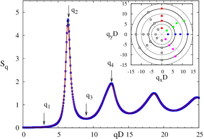
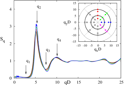
The equilibrium structure factor is the only input quantity to the MCT-ITT equations. It varies smoothly with density or temperature, but leads to the transition from a shear-thinning fluid to a yielding glassy state at a glass transition density . Figure 1 shows modified hyper-netted chain structure factors of monodisperse hard discs in from (Bayer et al. 2007) used in the MCT-ITT calculations. For comparison, the averaged structure factors obtained from the binary mixture simulation are shown also. In both cases, the value of the glass transition density is included in the curves in Fig. 1, and only smooth changes in are noticeable. The short range order at the average particle distance, as measured in the primary peak of , increases with densification. Differences in the structure between the mono- and the bidisperse system become appreciable beyond the primary peak, and especially beyond the second peak in . Also the height of the primary peak in at differs, indicating that the averaged structure factor in the bidisperse system does not well characterize the local structure and caging in the simpler system, and that a comparison with a bidisperse MCT-ITT calculation should be performed. As this is outside the present numerical reach, we proceed by comparing results for the characteristic wavevectors denoted to in Fig. 1. The angular dependence of the anisotropic structure will be explored along the special directions indicated in the insets.
5.2 Transient coherent density correlation functions
The central quantities in MCT-ITT, which encode the competition between shear driven motion and random fluctuations, are the transient density correlators. Structural rearrangements manifest themselves as a (second) slow relaxation process in the , whose relaxation time depends sensitively on the distance to the glass transition, measured by the (relative) separation parameter , and on the magnitude of the shear rate. Figure 2 shows representative curves in a fluid state (left column) and in a shear-melted glassy state (right column) for the wavevectors and directions defined in Fig. 1, and for nine different shear rates. The denoted bare Peclet numbers measure the shear rate compared to the Brownian diffusion time estimated with the single particle diffusion coefficient at infinite dilution. Characteristically, for the present strongly viscoelastic system, shear affects the structural relaxation already at extremely small bare Peclet numbers Pe. The short time motion, which corresponds to the local diffusion of the particles within their neighbour cages, however, is not much affected as long as Pe holds.
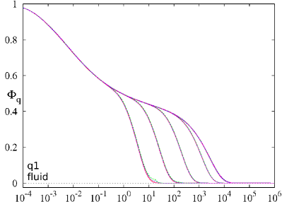
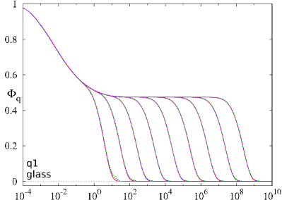
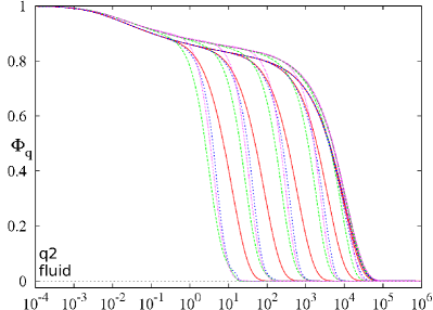
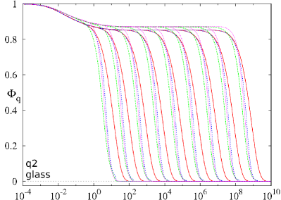
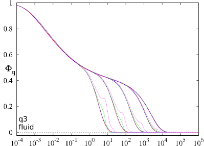
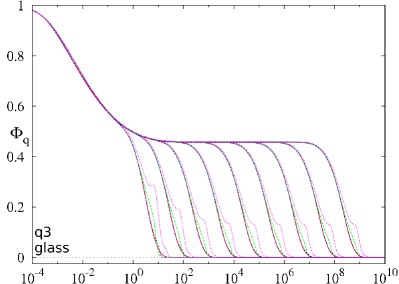
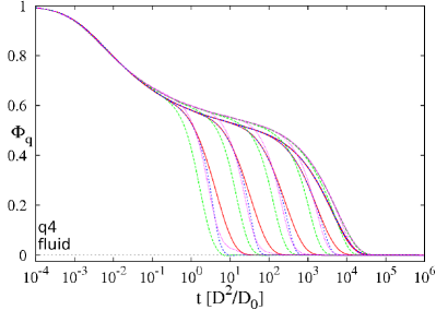
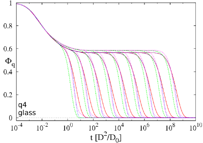
In the fluid (), a linear response regime, where shear does not affect the decay of thermal fluctuations, is observed for small (dressed) Peclet or Weissenberg numbers Pe, where Pe measures the shear rate relative to the intrinsic relaxation time. The latter can be estimated from the relaxation of , viz. at the primary peak of , where the structure relaxes most slowly in the quiescent case. The final (or -) relaxation time increases strongly when approaching the glass transition; with predicted by MCT (Bayer et al. 2007). For the fluid state in Fig. 2, only Pe is small enough that Pe holds and the final relaxation curves agree for different shear rates. In the glass (), shear is the origin of the decay of the otherwise frozen-in density fluctuations, and all nine shear rates lead to different final decays. While for small and larger wavevectors the final decay is rather isotropic, around the main peak in some anisotropy is noticeable in the transient correlators. In the direction perpendicular to the flow, (red), shear is not as efficient in decorrelating the density as in the other directions, which fall closer together.
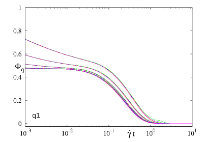
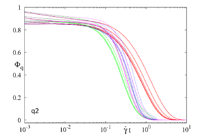
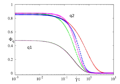
One of the central predictions of MCT-ITT concerns the existence of a scaling law describing the yielding of glassy states, which manifests itself by an approach to a master function for decreasing shear rate, and , where the rescaled time agrees with the accumulated strain. This scaling law, which is quite obvious in Fig. 2, is tested quantitatively for some wavevectors in Fig. 3, and holds extremely well (for ), or with pre-asymptotic corrections (for ). The shapes of the yielding master functions can be very well fitted with compressed exponentials, , but the parameters, including the exponent , depend on wavevector and orientation; see Table 1 for representative values.
| red | 3.0 | 0 | 3.0 | 0.479 | 1.121 | 0.255 |
| green | 3.0 | 2.4 | 1.8 | 0.481 | 1.117 | 0.263 |
| blue | 3.0 | 3.0 | 0 | 0.479 | 1.112 | 0.258 |
| magenta | 3.0 | 1.8 | -2.4 | 0.480 | 1.117 | 0.249 |
| red | 6.6 | 0 | 6.6 | 0.856 | 1.084 | 0.811 |
| green | 6.5 | 5.4 | 3.6 | 0.878 | 1.384 | 0.291 |
| blue | 6.6 | 6.6 | 0 | 0.875 | 1.670 | 0.363 |
| magenta | 6.5 | 3.6 | -5.4 | 0.849 | 1.617 | 0.431 |
The quite good fit to compressed exponentials is at present only a numerical observation. Yet, close to the glass transition asymptotic expansions are possible which analytically predict the initial part of the yield master functions (Fuchs Cates 2002,2003,2009):
As the critical glass form factor and the critical amplitude are isotropic, this result suggests a rather isotropic yielding process right at the glass transition density. Approximating by an exponential, it also provides an estimate for the final relaxation time under shear. Except for all quantities in the above formula have been determined in quiescent MCT (Bayer et al. 2007), and our values (e.g. ) differ only because of the coarser discretization in space that is necessary under shear. Close to the glass transition, we estimate . As the bottom left panel in Fig. 3 and Fig. 2 both show, this estimate for the final relaxation time is quite good close to the transition, but deeper in the glass the correlators become somewhat more anisotropic. Specifically for (red) with wavevector magnitudes around , the correlator slows down relative to other orientations.
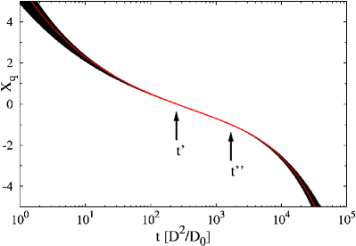
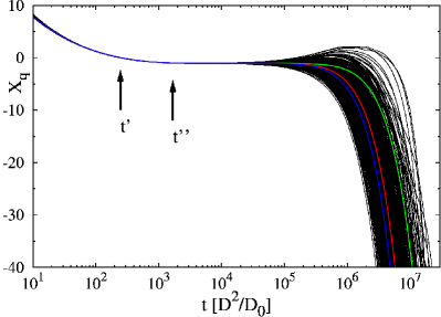
More detailed analytical predictions, are possible around , where spatial and temporal dependences in the transient fluctuations decouple (Fuchs Cates 2003):
is a universal function, which only depends on , and is another MCT time scale that diverges at the glass transition (Bayer et al. 2007). This factorization property known from quiescent MCT generalizes to steady shear, and is an essential feature of the localization transition that underlies glass formation in MCT. In Fig. 4, the quantity is plotted which should become wavevector and orientation independent if factorisation holds. This holds in the liquid, and in the glass, where however shear leads to strong (anisotropic) pre-asymptotic corrections already for .
6 Results and comparisons
Based on the approximated generalized Green-Kubo relations of Eqs. (12) and (13), and the properties of the transient correlators discussed in the previous section, MCT-ITT makes a number of predictions for stationary stresses and structural correlations (Fuchs Cates 2002, 2009). In the following, we will test these qualitatively, but also quantitatively, by comparing them to the two-dimensional simulation data.
6.1 Stationary stresses
The quantity of most interest in nonlinear rheology is the shear stress . Flow curves giving the shear stress as function of the shear rate can be obtained in the simulations and are shown in Fig. 5. The viscosity decreases below its Newtonian value upon increasing the shear rate already for small Pe0 values. Shear thinning in which the stress increases less than linearly with , sets in at Pe of the order of unity, and this crossover shifts to lower and lower Pe0 for increasing density. At the density around , the crossover leaves the accessible shear rate window. We use this as estimate of an ideal glass transition density, where the final relaxation time and the quiescent Newtonian viscosity () diverge. Moreover, at this density the flow curves change from a characteristic S shape in the fluid, to exhibiting a rather -independent plateau at small shear rates. This change is the hallmark of the transition in MCT-ITT between a shear thinning fluid and a yielding glass (Siebenbürger et al. 2009).
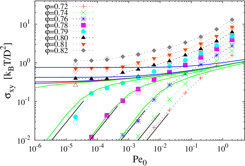
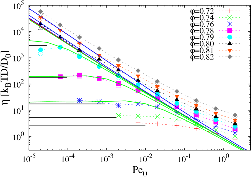
The numerical MCT-ITT solutions show the same transition scenario, but because of the approximations involved, exhibit a different critical density than the simulations. Even if theory and simulation considered the same (binary) system, a difference in critical packing fraction would be expected as is well known also in three dimensions (Voigtmann et al. 2004). Thus the following MCT-ITT calculations match the relative separation from in order to compare with the simulations. As MCT-ITT is aimed at describing the long time structural motion, errors need to be anticipated in its description of short time properties. This is obvious in real dispersions, where hydrodynamic interactions (neglected in MCT-ITT) affect the short time diffusion coefficient , but may arise in the following comparisons, also. A rescaling of the effective Peclet number Pe would correct for this change in . In order not to introduce additional fit parameters we refrain from doing so, but anticipate that future comparisons may require .
The approach to a yield scaling law, where the final decay of the
transient correlators depends on the accumulated strain only (see
Figs. 2 and 3), predicts the existence of a
(dynamical) yield stress
, which
characterizes the shear melted glass. In the bidisperse hard disc mixture, at the glass transition it takes the (critical) value ; below the glass transition, the yield stress jumps to zero, . Its quantitative prediction is
quite a challenge for theory, because Eq. 12 shows that
it requires an accurate calculation of the shear driven relaxation
process. MCT-ITT overestimates the critical yield stress
by roughly a factor 10 because,
presumably, the decay of the transient correlators is too slow. Yet,
of course the difference between the monodisperse system in the
MCT-ITT calculation and the bidisperse simulated system contributes
in unknown way to the error. It appears reasonable to
assume that mixing two species reduces the stresses under flow,
which would explain part of the deviation.
At larger shear rates, the flow curves from simulation appear to approach a second Newtonian
plateau which, presumably, strongly depends on
the hard-core character of excluded volume interactions and is outside the reach of the
present MCT-ITT. The latter, by using its sole input rather than pair potential, is not directly aware of hard-core constraints.
We checked, however, that the states remain
homogeneous and random up to the Pe0 values shown.
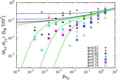
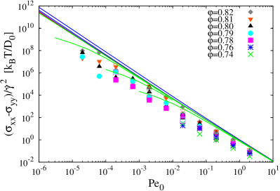
Reassuringly, the same rescaling factor of 0.1 as for the shear stress brings theoretical and simulational normal stress differences, , into register also; see Fig. 7. The normal stress differences are positive (indicating that the dispersion would swell after flowing through a nozzle), and show similar behavior to the stress, increasing like in the fluid for small shear rates, and leveling out onto a plateau in the yielding glass.
6.2 Distorted micro-structure
The macroscopic stresses in the flowing dispersion are experimentally most important, but provide only an averaged description of the local effects of shear. Spatially resolved information can be learned from the distorted structure factor , which in MCT-ITT is connected to the stress via
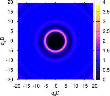
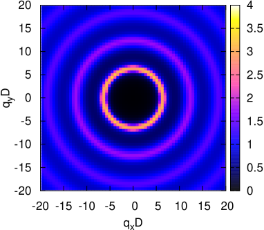
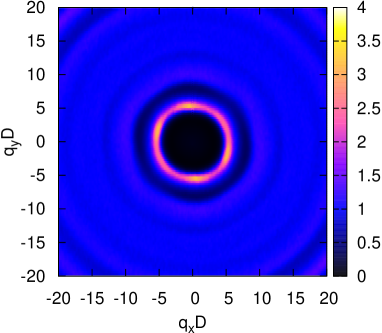
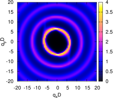
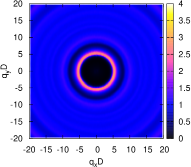
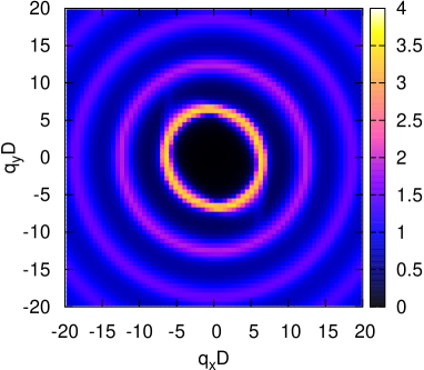
Figure 8 shows colour-coded structure factors as function of the two-dimensional wavevector , with in the direction of flow and along the gradient direction. In the left column, panels with simulation data are compared to panels in the right column obtained in MCT-ITT. Scattering intensities are presented (top row) in the linear response regime in the fluid, effectively measuring the equilibrium structure factors already shown in Fig. 1, (middle row) at high shear in the glass, where all densities are in the shear thinning region, and (bottom row) in the glass at low shear rate, where the yielding glassy state is tested. While the fluid is isotropic for small Pe0 (case ), as required by linear response theory, increasing Pe0 to values around unity, leads to an ellipsoidal scattering ring, which is elongated along the so-called ’compressional axis’ , and more narrow along the ’extensional axis’ ; this indicates that shear pushes particles together along the compressional and pulls particles apart along the extensional diagonals (Vermant Solomon 2005). Theory and simulation data in this representation qualitatively agree except for that MCT-ITT somewhat overestimates the anisotropic distortion of the glass structure at low Pe0.
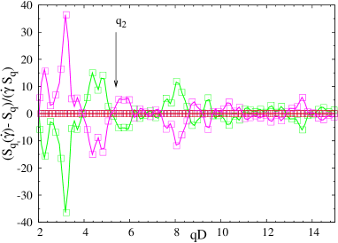
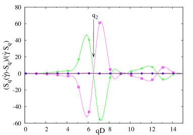
A more careful look onto the distorted microstructure is provided by -dependent cuts through along the directions colour-coded in Fig. 1. Important for the direction (red) is the need, present in both simulation and theory, to average over a small but finite angle, because exactly at the structure oscillates noisily around zero.
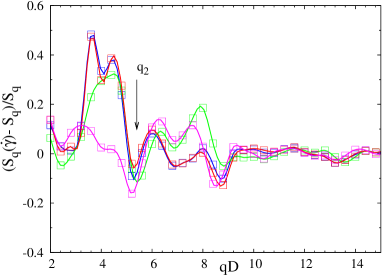
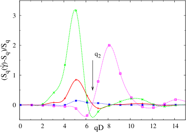
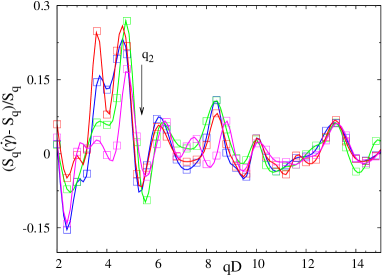
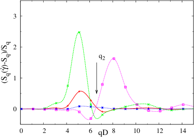
Especially of interest are the intensities of case , where the stationary structure of the shear melted solid is studied. The density is not yet high enough to lie in the glass, but close enough to the glass transition so that the correlations at quite low rate, namely Pe, closely resemble the ones of glassy states at very low shear rates. (While we can get good statistics for stresses at Pe for all densities, structure factors can not be sampled sufficiently there.) At this density of also the equilibrium structure factor can be obtained in long simulation runs, and the (relative) difference can thus be determined. It is shown in Fig. 9 for two states in order to investigate the distorted structure of the shear melted glass in detail. We base the following discussion on the hypothesis that Pe at captures a glass-like state in the limit of low bare Peclet number.
Figure 9 provides a sensitive test of the accuracy of the theoretical predictions. The lower left panel shows that the structure factor at vanishing shear rate jumps discontinuously at the glass transition; while holds in the fluid, holds in the glass. Relative deviations of 20% remain. Simulation finds quite isotropic deviations which show a maximum on the low- side of the primary peak in . MCT-ITT predicts the absence of a linear response regime in as function of the shear rate in the glass, and derives it from the existence of the yield scaling law in the transient correlators. Because sets the time scale for the final relaxation into the stationary state, the limit does not agree with the quiescent result .
Quantitatively, MCT-ITT overestimates the distortion again by a factor up to 10, and finds a noticeable anisotropy, as discussed in context with Fig. 8. While the difference between the bidisperse and the monodisperse system may influence the comparison, we believe that the major origin of the error is that MCT-ITT underestimates the speeding up of structural rearrangements caused by shear. The too slow transient correlators thus become anisotropic because the accumulated strain becomes too big before structural correlations have decayed.
Qualitatively, aspects of the anisotropy predicted by MCT-ITT can be seen in the simulations at only slightly larger shear rates, like at Pe shown in the middle left panel of Fig. 9. While along the two axis- and the extensional diagonal direction, the low- wing of the primary peak in becomes enhanced under shear, along the compressional axis (magenta) it gets suppressed, and the high- wing is pushed up. Simulation also finds a suppression of the peak height along all directions, which MCT-ITT reproduces along the diagonal directions. Overall the anisotropy and the magnitude of the distortions predicted by MCT-ITT remain too large, but the deviation decreases. The differences between the equilibrium structure factors in the simulated and in the calculated system should be taken into account in future work, and presently preclude comparisons at larger wavevectors.
7 Conclusions and Outlook
The first fully quantitative solutions of the MCT-ITT equations for the distorted microstructure and the stresses in steadily sheared two-dimensional shear-thinning fluids and yielding glasses of Brownian hard discs exhibit all the universal features discussed within schematic MCT-ITT models (Fuchs Cates 2003). They compare qualitatively well, but quantitatively with appreciable errors, with Brownian dynamics simulations of a bidisperse mixture without hydrodynamic interactions in a linear shear profile, which for all states considered remains in an homogeneous and disordered state. The non-analytic behavior of the stationary properties, and the lack of a linear response regime throughout the (shear-melted) glass state, predicted by theory, can be found in the simulation.
Acknowledgements
Work funded in part by DFG-IRTG 667, and EPSRC grants EP/045316 and EP/030173. MEC holds a Royal Society Research Professorship
References
- [1]
- [2] Alder B. J., Gass D. M. Wainwright T. E. 1970 J. Chem. Phys. 53 3813.
- [3]
- [4] Bayer, M., Brader, F. Ebert, E. Lange, M. Fuchs, G. Maret, R. Schilling, M. Sperl, Wittmer, J. P. 2007 Phys. Rev. E 76 011508.
- [5]
- [6] Brader, J., Cates, M. E Fuchs, M. 2008 Phys. Rev. Lett. 101 138301.
- [7]
- [8] Foss, D. R. Brady, J. F. 2000 J. Rheol 44 629-651.
- [9]
- [10] Fuchs, M. Cates, M. E. 2002 Phys. Rev. Lett. 89 248304.
- [11]
- [12] Fuchs, M. Cates, M. E. 2002 Faraday Discuss. 123 267-286.
- [13]
- [14] Fuchs, M. Cates, M. E. 2009 , J. Rheol. 53(4) 957-1000.
- [15]
- [16] Furukawa, A., Kim, K., Saito, S. Tanaka, H. 2009 Phys. Rev. Lett. 102 016001.
- [17]
- [18] Lange, E., Caballero, J. B., Puertas, A. M. Fuchs, M. 2008 J. Chem. Phys. 130 174903
- [19]
- [20] Miyazaki K., Reichmann D. R. Yamamoto, R. 2004 Phys. Rev. E 70 011501.
- [21]
- [22] Ng, K.-C. 1974 J. Chem. Phys. 61 2680-2689.
- [23]
- [24] Petekidis, G., Moussaïd, A. Pusey, P. N. 2002 Phys. Rev. E 66 051402.
- [25]
- [26] Scala, A., Voigtmann, T. De Michele, C. 2007 J. Chem. Phys. 126 134109.
- [27]
- [28] Strating, P. 1999 Phys. Rev. E 59 2175.
- [29]
- [30] Siebenbürger, M., Fuchs, M., Winter, H. H. Ballauff, M. 2009 J. Rheol 53 707-726.
- [31]
- [32] Vermant, J. Solomon, M. J. 2005 J. Phys.: Condens. Matter 17 R187-R216
- [33]
- [34] Voigtmann, Th., Puertas, A. M. M. Fuchs 2004 Phys. Rev. E 70 061506.
- [35]
- [36] Yamamoto, R. Onuki, A. 1998 Phys. Rev. E 58 3515-3529.