Polymer heat transport enhancement in thermal convection: the case of Rayleigh-Taylor turbulence

Abstract

We study the effects of polymer additives on turbulence generated by the ubiquitous Rayleigh-Taylor instability. Numerical simulations of complete viscoelastic models provide clear evidence that the heat transport is enhanced up to $50\%$ with respect to the Newtonian case. This phenomenon is accompanied by a speed up of the mixing layer growth. We give a phenomenological interpretation of these results based on small-scale turbulent reduction induced by polymers.

Controlling transport properties in a turbulent flow is an issue of paramount importance in a variety of situations ranging from pure sciences to technological applications Gad-el-Hak (2000); Siggia (1994); Warnatz et al. (2001). After Toms Toms (1949), one of the most spectacular way to achieve this goal consists in adding inside the fluid solvent a small amount of long-chain polymers (parts per million by weight). The resulting fluid solution acquires a non-Newtonian character and the most interesting dynamical effect played by polymers is encoded in the drag coefficient, a dimensionless measure of the power needed to maintain a given throughput in a pipe. With respect the Newtonian case (i.e., in the absence of polymers), it can be reduced up to $80\%$ Lumley (1969); Sreenivasan and White (2000).

In many relevant situations (e.g. atmospheric convection) the velocity field is two-way coupled to the temperature field with the result that, together with mass, also heat is transported by the flow. Because drag reduction is associated to mass transport enhancement, an intriguing question is on whether this is accompanied by a similar variation in the heat transport.

In this Letter we demonstrate the simultaneous occurrence of mass transport enhancement (drag reduction) and heat transport enhancement induced by polymers in a three-dimensional buoyancy driven turbulent flow originated by the ubiquitous Rayleigh–Taylor (RT) instability Rayleigh (1883); Taylor (1950). This instability arises at the interface between a layer of light fluid and a layer of heavy fluid placed above and develops in a turbulent mixing layer (see Fig. 1) which grows accelerated in time. Heuristically, the RT system can be assimilated to a channel inside which vertical motion of thermal plumes is maintained by the available potential energy. Our idea on the possibility of observing drag reduction in this system is suggested by recent analytical results which show a speed-up of the instability due to polymer additives Boffetta et al. (2010). Moreover, examples of turbulent drag reduction without boundaries have been recently provided, e.g., in Benzi et al. (2003); De Angelys et al. (2005); Berti et al. (2006); Boffetta et al. (2005)

Direct numerical simulations of primitive equations show that thermal plumes are faster in the presence of polymers (see Fig. 1), therefore the mixing layer accelerates (up to $30\%$ at final observation time) with respect to the Newtonian case and complete mixing is achieved in a shorter time. A second and more dramatic effect, also clearly detectable in Fig. 1, is that polymers reduce small scale turbulence Benzi et al. (2003); De Angelys et al. (2005); Berti et al. (2006). As a consequence, thermal plumes in the viscoelastic case are more coherent and transport heat more efficiently. Quantitatively, the enhancement of the heat transport corresponds to larger values (more than $50\%$ at final observation time) of the Nusselt number with respect the Newtonian case.

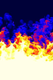
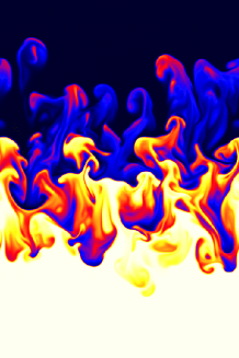
Figure 1: Vertical sections of temperature field for Newtonian (left) and viscoelastic (right) RT simulation at time $t=2\tau$ starting from the same initial conditions. White (black) regions correspond to hot (cold) fluid. Boussinesq-Oldroyd-B equations (1) are integrated by a standard fully dealiased pseudo-spectral code on uniform grid at resolution $512\times 512\times 1024$. Physical parameters are $Pr=\nu/\kappa=1$, $\eta=0.2$ ($\eta=0$ for Newtonian run), $\beta g=0.5$, $\theta_{0}=1$ ($Ag=0.25$). Deborah number $De=\tau_{p}/\tau$ is $De=0.2$. The initial perturbation is seeded in both cases by adding a $10\%$ of white noise (same realization for both runs) to the initial temperature profile in a small layer around the middle plane $z=0$.

We consider the incompressible RT system in the Boussinesq approximation generalized to a viscoelastic fluid using the standard Oldroyd-B model Bird et al. (1987)

$$\begin{array}[]{lll}\partial_{t}{\bf u}+{\bf u}\cdot{\bf\nabla}{\bf u}&=&-{\bf\nabla}p+\nu\nabla^{2}{\bf u}-\beta{\bf g}T+{2\nu\eta\over\tau_{p}}{\bf\nabla}\cdot\sigma\\ \partial T+{\bf u}\cdot{\bf\nabla}T&=&\kappa\nabla^{2}T\\ \partial_{t}\sigma+{\bf u}\cdot{\bf\nabla}\sigma&=&({\bf\nabla}{\bf u})^{T}\cdot\sigma+\sigma\cdot({\bf\nabla}{\bf u})-{2\over\tau_{p}}(\sigma-\mathbb{I})\end{array}$$ (1)

together with the incompressibility condition ${\bf\nabla}\cdot{\bf u}=0$. In (1) $T({\bf x},t)$ is the temperature field, proportional to the density via the thermal expansion coefficient $\beta$ as $\rho=\rho_{0}[1-\beta(T-T_{0})]$ ($\rho_{0}$ and $T_{0}$ are reference values), $\sigma_{ij}({\bf x},t)$ is the positive symmetric conformation tensor of polymer molecules, ${\bf g}=(0,0,-g)$ is gravity acceleration, $\nu$ is the kinematic viscosity, $\kappa$ is the thermal diffusivity, $\eta$ is the zero-shear polymer contribution to viscosity (proportional to polymer concentration) and $\tau_{p}$ is the (longest) polymer relaxation time Bird et al. (1987).

The initial condition for the RT problem is an unstable temperature jump $T({\bf x},0)=-(\theta_{0}/2)sgn(z)$ in a fluid at rest ${\bf u}({\bf x},0)=0$ and coiled polymers $\sigma({\bf x},0)=\mathbb{I}$. The physical assumptions under which the set of equations (1) is valid are of small Atwood number $A=(1/2)\beta\theta_{0}$ (dimensionless density fluctuations) and dilute polymer solution. Experimentally, density fluctuations can also be obtained by some additives (e.g., salts) instead of temperature fluctuations: within the validity of Boussinesq approximation, these situations are described by the same set of equations (1). In the following, all physical quantities are made dimensionless using the vertical side, $L_{z}$, of the computational domain, the temperature jump $\theta_{0}$ and the characteristic time $\tau=(L_{z}/Ag)^{1/2}$ as fundamental units. Elasticity of the polymer solution is measured by the Deborah number $De$, the ratio of polymer relaxation time to a characteristic time of the flow. In our unsteady case $De$ grows in time starting from $De=0$, therefore viscoelastic effects are initially absent. An estimate of the largest Deborah number achievable is based on the large scale convective time as $De=\tau_{p}/\tau$.

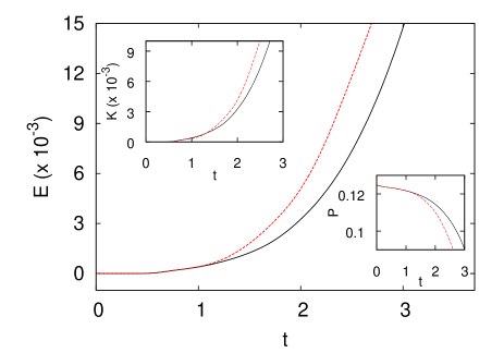
Figure 2: Time evolution of total energy $E=K+\Sigma$, kinetic energy $K$ (upper inset) and potential energy $P$ (lower inset) for the Newtonian run ($De=0$, black continuous line) and the viscoelastic run ($De=0.2$, red dashed line).

Total energy of the solution has an additional elastic contribution to kinetic energy $E=K+\Sigma=(1/2)\langle u^{2}\rangle+(\nu\eta/\tau_{p})\langle tr\sigma\rangle$ and the energy balance for (1) reads

$$-{dP\over dt}=\beta g\langle wT\rangle={dE\over dt}+\varepsilon_{\nu}+{2\nu\eta\over\tau_{p}^{2}}\left[\langle tr\sigma\rangle-3\right]$$ (2)

where $P=-\beta g\langle zT\rangle$ is the potential energy and $\varepsilon_{\nu}=\nu\langle(\partial_{\alpha}u_{\beta})^{2}\rangle$ is the viscous dissipation and the last term represents elastic dissipation. Because this last term in (2) is not negative, one might expect that the presence of polymers accelerates the consumption of potential energy with respect to the Newtonian case ($\eta=0$), as it is indeed observed in Fig. 2.

Of course, the speed-up of potential energy consumption due to polymers does not automatically imply the increase of kinetic energy growth. Part of potential energy is indeed converted to elastic energy $\Sigma$ by polymers elongation. The inset of Fig. 2 shows indeed that kinetic energy for viscoelastic runs is larger than in the Newtonian case (of about $40\%$ at $t=2.5\tau$). This is the fingerprint of a “drag reduction” as defined for homogeneous-isotropic turbulence in the absence of a mean flow Benzi et al. (2003); De Angelys et al. (2005).

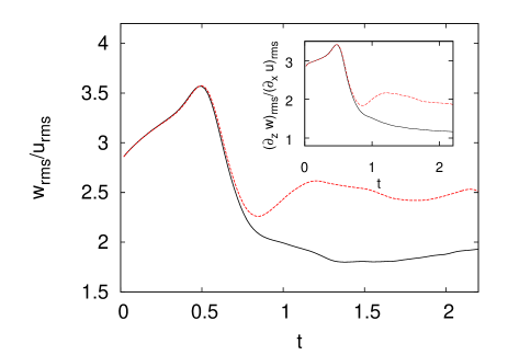
Figure 3: Time evolution of velocity anisotropy $w_{rms}/u_{rms}$ where $w$ and $u$ are the vertical and one horizontal velocity components, respectively. Black line is the Newtonian run at $De=0$, red dashed line is the viscoelastic run at $De=0.2$. Inset: the evolution of the ratio of velocity gradients $(\partial_{z}w)_{rms}/(\partial_{x}u)_{rms}$.

The most important effect of polymers on turbulent velocity is to generate more coherent thermal plume with respect the Newtonian case, as it is evident in Fig. 1. This reflects in larger vertical component of the velocity with respect the horizontal one, i.e., an increased anisotropy of the velocity field. This effect is evident in Fig. 3 where we plot the ratio of vertical rms velocity $w_{rms}$ to horizontal one $u_{rms}$. The anisotropy ratio, which is around $1.8$ for the Newtonian case Boffetta et al. (2009), becomes larger than $2.5$ for the viscoelastic run. More important, in the viscoelastic case the anisotropy persists also at small scales (i.e., in the ratio of velocity gradients), while it is almost absent in the Newtonian case (see inset of Fig. 3).

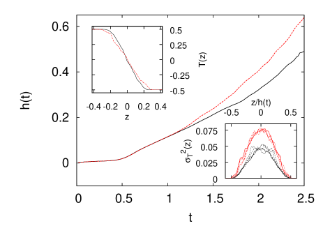
Figure 4: Growth of the mixing layer thickness $h_{0.98}(t)$ defined as the vertical range for which $|\overline{T}(z)|\leq 0.98\theta_{0}/2$ as a function of dimensionless time $t/\tau$ for Newtonian run (black line) and the viscoelastic run (dashed red line) starting from the same initial condition. Upper inset: mean temperature profiles $\overline{T}(z)$ for the two cases at time $t=2\tau$. Lower inset: temperature variance profiles $\sigma_{T}^{2}(z)$ at different times vs $z/h(t)$ (black Newtonian, red: viscoelastic run).

Despite the fact that RT turbulence has vanishing mean flow, a natural mean velocity is provided by the growth of the width $h(t)$ of the turbulent mixing layer where heavy and light fluids are well mixed. For ordinary fluids at small viscosity, as a consequence of constant acceleration, one expects $h(t)=\alpha Agt^{2}$ where $\alpha$ is a dimensionless parameter to be determined empirically Ramaprabhu and Andrews (2004); Dimonte et al. (2004); Kadau et al. (2007). Several definitions of $h(t)$ have been proposed, based on either local or global properties of the mean temperature profile $\overline{T}(z,t)$ (the overbar indicates average over the horizontal directions) Andrews and Spalding (1990); Dalziel et al. (1999); Cabot and Cook (2006); Vladimirova and Chertkov (2008). The simplest measure $h_{r}$ is based on the threshold value of $z$ at which $\overline{T}(z,t)$ reaches a fraction $r$ of the maximum value i.e. $\overline{T}(\pm h_{r}(t)/2,t)=\mp r\theta_{0}/2$.

Figure 4 shows the growth of the mixing layer thickness for both Newtonian and viscoelastic RT turbulence. As already suggested by Fig. 1, in the viscoelastic solution the growth of the mixing layer is faster than in the Newtonian case (i.e. larger $h(t)$, up to $30\%$ at $t=2.5\tau$), therefore we have an effect of polymer drag reduction, i.e. polymer addiction makes the transfer of mass more efficient. The inset of Fig. 4 shows that the increased efficiency is a global property of the mixing layer and the temperature profile of the viscoelastic solution corresponds to the profile of the Newtonian case at a later time.

Also in Fig. 4 we plot the variance profiles of temperature field computed at different times for both Newtonian and viscoelastic turbulence. In both cases, $\sigma_{T}^{2}(z)$ at different times collapse when plotted as a function of rescaled variable $z/h(t)$. Therefore as turbulence develops in the domain, the level of temperature fluctuations within the mixing layer remains constant as a consequence of new fluctuations introduced by plumes entering from unmixed regions. As Fig. 4 indicates, the level of fluctuations is larger in the viscoelastic case, as a consequence of the reduced mixing at small scales (already observed in Fig. 1). We remark that all together these results are consistent with the accepted phenomenology of viscoelastic homogeneous-isotropic turbulence where polymers simultaneously reduce energy at small scales and enhance energy contain at large scales Benzi et al. (2003); De Angelys et al. (2005); Berti et al. (2006).

The turbulent mixing layer is responsible for the huge enhancement of the heat exchange with respect to the steady conductive case. The dimensionless measure of the heat transport efficiency is usually given by the Nusselt number $Nu=\langle wT\rangle h/(\kappa\theta_{0})$, the ratio between convective and conductive heat transport. For a convective flow in the fully developed turbulent regime, the Nusselt number is expected to behave as a simple scaling law with respect to the dimensionless temperature jump which defines the Rayleigh number $Ra=Agh^{3}/(\nu\kappa)$ Grossmann and Lohse (2000). For a flow in which boundary layers are irrelevant, as in our case, Kraichnan predicted many years ago the so-called ultimate state of thermal convection for which (a part logarithmic corrections) Kraichnan (1962); Grossmann and Lohse (2000)

$$\begin{array}[]{c}Nu=CPr^{1/2}Ra^{1/2}\\ Re=DPr^{-1/2}Ra^{1/2}\end{array}$$ (3)

where $C$ and $D$ are numerical coefficients. The ultimate state regime has indeed recently been observed in numerical simulations of RT turbulence both in two and three dimensions Celani et al. (2006); Boffetta et al. (2009, in press, 2010).

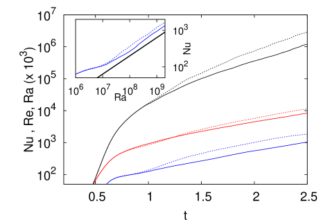
Figure 5: Time evolution of Nusselt number $Nu=\langle wT\rangle/(\kappa\theta_{0})$ (blue, lower lines), Reynolds number $Re=u_{rms}h/\nu$ (red, intermediate lines) and Rayleigh number $Ra=Agh^{3}/(\nu\kappa)$ (black, upper lines) for the Newtonian run (continuous lines) and the viscoelastic run (dotted lines).

In Fig. 5 we show the evolution of the Rayleigh number $Ra$, the Nusselt number $Nu$ and the Reynolds number $Re=u_{rms}h/\nu$ as a function of time. For $t\geq\tau$, when turbulence is developed, all these dimensionless quantities grow following dimensional predictions, i.e. $Ra\sim t^{6}$ and $Nu\sim Re\sim t^{3}$. Moreover, it is evident that the effect of polymers is to increase the values attained by those quantities at late time. Of course, most of this effect is due to the enhanced value, for the viscoelastic solution, of the width $h(t)$ of the mixing layer which enters in the definition of all the quantities. As discussed before, another effect induced by polymers is the reduction of small-scale turbulence in the thermal plumes, which leads to an additional enhancement for the heat flux $\langle wT\rangle$. Therefore, the Nusselt number for viscoelastic turbulence is expected to increase with respect to the Newtonian case when it is observed both as a function of time and as a function of $Ra$. Indeed, as shown in the inset of Fig. 5, both in the Newtonian and in the viscoelastic cases, $Nu\simeq Ra^{1/2}$ in agreement with the ultimate state regime (3) but with different coefficients, $C_{N}=0.022\pm 0.002$ and $C_{VE}=0.028\pm 0.002$ respectively, corresponding to an increases of $27\%$.

In conclusion, we have exploited high resolution direct numerical simulations to investigate the effects of polymer additives on Rayleigh-Taylor turbulence. There are several advantages in using the present buoyancy-driven turbulence system. The presence of a time evolving mixing layer allows us to quantify the acceleration induced by polymers on a natural (nonzero) mean velocity (the mixing layer growth velocity) at fixed buoyancy forcing, exactly in the same spirit of usual drag reduction in bounded flows. The relative simple and well understood phenomenology of the heat transport (which follows the Kraichnan’s ultimate state regime) allows us to quantify the effects of polymers on the heat transport. While the former feature is specific of the present configuration, the latter occurs in the bulk of the mixing region and therefore we conjecture that our findings hold in situations more general than the specific setup we studied, as indeed a recent investigation seems to indicate Benzi et al. (2010). Moreover, RT turbulence can be realized in laboratory experiments and therefore our results based on numerical simulations of primitive equations are a starting point of the experimental investigation of polymer additive effects on buoyancy-driven turbulent systems.

We thank the Cineca Supercomputing Center (Bologna, Italy) for the allocation of computational resources.

References

- Gad-el-Hak (2000) M. Gad-el-Hak, Flow control: passive, active, and reactive flow management (Cambridge University Press, 2000).
- Siggia (1994) E. Siggia, Ann. Rev. Fluid Mech. 26, 137 (1994).
- Warnatz et al. (2001) J. Warnatz, U. Maas, and R. W. Dibble, Combustion: Physical and Chemical Fundamentals, Modeling and Simulation, Experiments, Pollutant Formation. (Springer, New York, 2001).
- Toms (1949) B. A. Toms, Proc. 1st International Congress on Rheology 2, 135 (1949).
- Lumley (1969) J. L. Lumley, Ann. Rev. Fluid Mech. 1, 367 (1969).
- Sreenivasan and White (2000) K. R. Sreenivasan and M. C. White, J. Fluid Mech. 409, 149 (2000).
- Rayleigh (1883) L. Rayleigh, Proc. London. Math. Soc 14, 170 (1883).
- Taylor (1950) G. Taylor, Proc. Royal Soc. London 201, 192 (1950).
- Boffetta et al. (2010) G. Boffetta, A. Mazzino, S. Musacchio, and L. Vozella, J. Fluid Mech. 643, 127 (2010).
- Benzi et al. (2003) R. Benzi, E. De Angelis, R. Govindarajan, and I. Procaccia, Phys. Rev. E 68, 016308 (2003).
- De Angelys et al. (2005) E. De Angelys, C. M. Casciola, R. Benzi, and R. Piva, J. Fluid Mech. 531, 1 (2005).
- Berti et al. (2006) S. Berti, A. Bistagnino, G. Boffetta, A. Celani, and S. Musacchio, EPL (Europhysics Letters) 76, 63 (2006).
- Boffetta et al. (2005) G. Boffetta, A. Celani, and A. Mazzino, Phys Rev E 71, 036307 (2005).
- Bird et al. (1987) R. B. Bird, O. Hassager, R. C. Armstrong, and C. F. Curtiss, Dynamics of Polymeric Liquids (Wiley-Interscience, 1987).
- Boffetta et al. (2009) G. Boffetta, A. Mazzino, S. Musacchio, and L. Vozella, Phys. Rev. E 79, 065301 (2009).
- Ramaprabhu and Andrews (2004) P. Ramaprabhu and M. Andrews, Physics of Fluids 16, L59 (2004).
- Dimonte et al. (2004) G. Dimonte, D. L. Youngs, A. Dimits, S. Weber, M. Marinak, S. Wunsch, C. Garasi, A. Robinson, M. J. Andrews, P. Ramaprabhu, et al., Physics of Fluids 16, 1668 (2004).
- Kadau et al. (2007) K. Kadau, C. Rosenblatt, J. L. Barber, T. C. Germann, Z. Huang, P. Carlès, and B. J. Alder, Proc. Nat. Acad. Sci. 104, 7741 (2007).
- Andrews and Spalding (1990) M. J. Andrews and D. B. Spalding, Physics of Fluids A: Fluid Dynamics 2, 922 (1990).
- Dalziel et al. (1999) S. Dalziel, P. Linden, and D. Youngs, J. Fluid Mech. 399, 1 (1999).
- Cabot and Cook (2006) W. H. Cabot and A. W. Cook, Nature Physics 2, 562 (2006).
- Vladimirova and Chertkov (2008) N. Vladimirova and M. Chertkov, Phys. Fluids 21, 015102 (2008).
- Grossmann and Lohse (2000) S. Grossmann and D. Lohse, J. Fluid Mech. 407, 27 (2000).
- Kraichnan (1962) R. H. Kraichnan, Phys. Fluids 5, 1374 (1962).
- Celani et al. (2006) A. Celani, A. Mazzino, and L. Vozella, Phys. Rev. Lett. 96, 134504 (2006).
- Boffetta et al. (in press, 2010) G. Boffetta, F. De Lillo, and S. Musacchio, Phys. Rev. Lett. (in press, 2010).
- Benzi et al. (2010) R. Benzi, E. S. C. Ching, and E. De Angelis, Phys. Rev. Lett. 104, 024502 (2010).