Eigenphase preserving two-channel SUSY transformations

Abstract

We propose a new kind of supersymmetric (SUSY) transformation in the case of the two-channel scattering problem with equal thresholds, for partial waves of the same parity. This two-fold transformation is based on two imaginary factorization energies with opposite signs and with mutually conjugated factorization solutions. We call it an eigenphase preserving SUSY transformation as it relates two Hamiltonians, the scattering matrices of which have identical eigenphase shifts. In contrast to known phase-equivalent transformations, the mixing parameter is modified by the eigenphase preserving transformation.

, , ,

March 15, 2024

1 Introduction

The present work is a continuation of our previous investigations on supersymmetric (SUSY) transformations applied to coupled-channel problems with equal thresholds [1]. Our main aim here is to present a method based on SUSY transformations, which allows to construct potentials with given scattering properties, i.e., to solve an inverse scattering coupled-channel problem.

There are several approaches to this problem based on the Gelfand-Levitan-Marchenko methods [2, 3]. In particular, Newton, Jost and Fulton [4]-[6] generalized the Gelfand-Levitan method and solved the corresponding integral equations in the case of two channels and rational scattering ($S$) matrices. Exactly solvable coupled-channel potentials obtained by this technique may be used for describing the neutron-proton scattering. In particular, in this way, Newton and Fulton [6] constructed a three-parameter phenomenological neutron-proton potential fitting low-energy scattering data. It would be interesting to extend this result by enlarging the number of parameters to fit scattering data on a wider energy range; however, the method based on integral transformations is rather involved and therefore quite difficult to generalize. Using the Marchenko equation, the results of Newton and Fulton were nevertheless reproduced and improved by von Geramb et al[7]. A review of the present state of the art in the inverse scattering methods may be found in [8]-[11].

Our hope that the SUSY technique may be efficient for the multichannel Schrödinger equation is based on the well known equivalence between SUSY transformations and the integral transformations of the inverse scattering method for single-channel problems [12]-[15]. Due to this equivalence, one can use chains of first-order SUSY operators (also referred to as first-order Darboux differential operators [16]) for constructing a Hamiltonian with given scattering properties [17, 18]. This approach to the scattering inversion is more efficient [15] just because of the differential character of the transformation. There are several papers devoted to supersymmetric transformations for multichannel problems [19]-[26] (see also [27]-[30] for additional motivations and physical applications). Arbitrary chains of first-order SUSY transformations in the case of a matrix Schrödinger equation are studied in [31]. There, a matrix generalization of the well-known Crum-Krein formula is obtained. Another important ingredient of the supersymmetric inversion technique are the phase-equivalent SUSY transformations, which are based on two-fold, or second-order, differential operators. These are described in [32]-[34] for the single-channel case and in [24, 25] for the coupled-channel case. Such transformations keep the scattering matrix unchanged and simultaneously allow to reproduce given bound state properties.

It should be noted that methods based on a direct generalization of the SUSY technique to the multichannel case are not able to provide an easy control of the scattering properties for all channels simultaneously. For instance, in the two-channel case, the $S$-matrix is parametrized by the eigenphase shifts $\delta_{1}(k)$, $\delta_{2}(k)$ and mixing parameter $\epsilon(k)$, where $k$ is the wave number. Usual SUSY transformations modify these three quantities in a complicated way, which makes their individual control difficult. We believe that this is the reason why SUSY transformations did not find a wide application to multichannel scattering inversion.

In the present paper, we propose a two-fold SUSY transformation which allows us to modify $\epsilon(k)$ only, while keeping $\delta_{1}(k)$ and $\delta_{2}(k)$ unchanged. We call such a transformation eigenphase preserving. It is necessary to stress the difference between this new kind of transformation and the well-known phase-equivalent transformations mentioned above. A phase-equivalent transformation does not modify the scattering matrix at all, whereas the eigenphase preserving transformation modifies the mixing between channels. An important consequence of that is the possibility to use single channel SUSY transformations to fit experimental values of the eigenphase shifts. Afterwards, the mixing parameter can be fitted without further modification of the eigenphase shifts. Thus, the main advantage of our approach consists in splitting the inversion problem into two independent parts: (i) fitting eigenphase shifts to experimental values independently for each channel and (ii) fitting the mixing parameter between these channels. To solve the first problem, one can use the single-channel tools mentioned above. In the present work, we propose an elegant solution to the second problem.

In what follows, we will use definitions and notations introduced in our previous paper [1], where a first order coupling SUSY transformation is analyzed in details. Nevertheless, in section 2, we recall some basic formulae necessary in the next sections. In section 3, we describe the new two-fold SUSY transformation and prove our main result that this transformation preserves the eigenphase shifts. A simple illustrative example of an exactly-solvable coupled-channel potential with a given scattering matrix is presented in section 4. In the conclusion, we discuss possible applications of the presented method and formulate some possible lines of future investigations.

2 Two channel scattering with equal thresholds

Consider the two component radial Schrödinger equation [35, 36]

$$H_{0}\psi_{0}(k,r)=k^{2}\psi_{0}(k,r),\quad r\in[0,\infty)$$ (1)

with the Hamiltonian

$$H_{0}=-\mathbf{1}\frac{d^{2}}{dr^{2}}+V^{\mathrm{int}}_{0}(r)+l(l+\mathbf{1})r^{-2},\qquad l=\mbox{\rm diag}(l_{1},l_{2})\,.$$ (2)

Here $\mathbf{1}$ is the $2\times 2$ identity matrix and the interaction potential $V^{\mathrm{int}}_{0}(r)$ is a real and symmetric matrix, exponentially decreasing at large distances. We will consider the case of two partial waves $l_{1}$ and $l_{2}$ with identical parity,

$$l_{2}=l_{1}+2m,\qquad m\in\mathbb{Z}.$$ (3)

For the sake of convenience, we combine interaction $V^{\mathrm{int}}_{0}(r)$ and the centrifugal term into a single potential matrix $V_{0}(r)=V^{\mathrm{int}}_{0}(r)+l(l+\mathbf{1})r^{-2}$. To characterize this potential near the origin, we use a matrix singularity index $\nu$. Matrix $\nu$ is determined by the asymptotic behaviour of the potential near the origin,

$$V_{0}(r\rightarrow 0)=\nu(\nu+\mathbf{1})r^{-2}+{\rm O}(1)\,.$$ (4)

Below, only potentials with singularity index being a diagonal matrix with integer entries $\nu=\mbox{\rm diag}(\nu_{1},\nu_{2})$ and $\nu_{j}\geq l_{j}$ are considered. We will call such potentials physical and restrict ourselves to SUSY transformations that produce physical potentials.

As usual, the Jost solutions $f_{0}(k,r)$ are defined as matrix solutions of (1) with exponential asymptotic behaviour at large distances [35, 36]. In what follows, we will need a more detailed asymptotic behaviour of these solutions; it is given by the asymptotic behaviour of the Bessel functions of the third kind, $H_{l+\frac{1}{2}}^{(1)}(z)$, also called the first Hankel functions (see [37] for a definition). At large distances, the Jost solution thus behaves like the corresponding solution for the free particle

$$f_{0}(k,r\rightarrow\infty)\to{\rm diag}\left[h_{l_{1}}(kr),h_{l_{2}}(kr)\right]\,,\qquad h_{l}(z)=i^{l+1}\left(\frac{\pi z}{2}\right)^{\frac{1}{2}}H_{l+\frac{1}{2}}^{(1)}(z)$$ (5)

with

$$h_{l}(z\rightarrow\infty)=e^{iz}\left(1+\frac{i\Lambda}{2z}+{\rm o}(z^{-1})\right),\qquad\Lambda=l(l+1).$$ (6)

A special linear combination of the Jost solutions gives the regular solution

$$\varphi_{0}(k,r)=\frac{i}{2k}\left[f_{0}(-k,r)F_{0}(k)-f_{0}(k,r)F_{0}(-k)\right],$$ (7)

$$\varphi_{0}(k,r\rightarrow 0)\to{\mbox{\rm diag}}\left(\frac{r^{\nu_{1}+1}}{(2\nu_{1}+1)!!},\frac{r^{\nu_{2}+1}}{(2\nu_{2}+1)!!}\right)\,,$$ (8)

where matrix $F_{0}(k)$ is the so-called Jost matrix.

To construct eigenphase preserving transformations, we need solutions of the Schrödinger equation (1) with a special behaviour both at large distances and near the origin. Thus, we first prove that the necessary solutions exist.

Lemma 1.

For any momentum $k$ such that Im $k>0$, det $F_{0}(k)\neq 0$, and for any constants $c_{1,2},d_{1,2}\in\mathbb{C}$, there exist two vector solutions $\vec{u}(k,r)$ and $\vec{v}(k,r)$ of the Schrödinger equation (1) which behave at large distances as

$$\vec{u}(k,r\rightarrow\infty)={\rm e}^{-ikr}(c_{1},c_{2})^{T}(1+{\rm o}(1))\,,$$ (9)

$$\vec{v}(k,r\rightarrow\infty)={\rm e}^{ikr}(d_{1},d_{2})^{T}(1+{\rm o}(1))\,,$$ (10)

and near the origin as

$$\vec{u}(k,r\rightarrow 0)=(a_{1}r^{\nu_{1}+1},a_{2}r^{\nu_{2}+1})^{T}(1+{\rm o}(r))\,,$$ (11)

$$\vec{v}(k,r\rightarrow 0)=(b_{1}r^{-\nu_{1}},b_{2}r^{-\nu_{2}})^{T}(1+{\rm o}(r))\,,$$ (12)

where $a_{1,2},b_{1,2}\in\mathbb{C}$.

Proof.

To obtain the behaviour (10), $\vec{v}(k,r)$ can be expressed in terms of the Jost solution

$$\vec{v}(k,r)=f_{0}(k,r)(d_{1},d_{2})^{T}.$$ (13)

Formula (12) follows from the behaviour of the Jost solution near the origin (see, e.g., [35]).

Taking into account that Im $k>0$, one gets from (7)

$$\varphi_{0}(k,r\rightarrow\infty)\rightarrow\frac{i}{2k}f_{0}(-k,r)F_{0}(k)\,.$$ (14)

Here, we omit the second term in (7) since it becomes negligible at large distances with respect to the first term. Thus, solution $\vec{u}(k,r)$ may be obtained as

$$\vec{u}(k,r)=\frac{2k}{i}\varphi_{0}(k,r)F_{0}^{-1}(k)(c_{1},c_{2})^{T}.$$ (15)

Formula (11) follows from (8). ∎

The $2\times 2$ scattering matrix $S_{0}(k)$ is expressed in terms of the Jost matrix as

$$S_{0}(k)=e^{il\frac{\pi}{2}}F_{0}(-k)F_{0}^{-1}(k)e^{il\frac{\pi}{2}}\,.$$ (16)

Being unitary and symmetric, $S_{0}(k)$ can be diagonalized by an energy dependent orthogonal matrix $R_{0}(k)$

$$R_{0}^{T}(k)S_{0}(k)R_{0}(k)=\mbox{\rm diag}\left(e^{2i\delta_{0;1}(k)},e^{2i\delta_{0;2}(k)}\right),$$ (17)

where $\delta_{0;j}$ are the eigenphase shifts and the angle $\epsilon_{0}$ entering matrix $R_{0}$ is called the mixing angle

$$\qquad R_{0}(k)=\left(\begin{array}[]{cc}\cos\epsilon_{0}(k)&-\sin\epsilon_{0}(k)\\ \sin\epsilon_{0}(k)&\cos\epsilon_{0}(k)\end{array}\right).$$ (18)

Note that an opposite sign definition for the mixing angle could have been chosen; moreover, the order of the eigenphase shifts is arbitrary: exchanging them while adding $\pm\pi/2$ to the mixing angle keeps the scattering matrix unchanged. In the next section, the eigenphase preserving SUSY transformations are defined.

3 Eigenphase preserving two-fold SUSY transformations

3.1 Two-fold SUSY transformations

Two-fold SUSY transformations lead to a number of interesting quantum models with unusual properties [38]. In particular, the corresponding superalgebra is nonlinear. It is natural to consider the two-fold SUSY transformation of the Schrödinger equation (1) as a chain of usual (i.e. one-fold) SUSY transformations. One-fold transformations for coupled-channel Schrödinger equations were introduced in [19]. Their generalization, which allows to introduce a coupling between channels, was given in [1]. The additional requirement that the transformed potential be physical was shown to result in a strong constraint on the transformation parameters. The case of two transformations is less restrictive since the intermediate Hamiltonian may be chosen unphysical. In particular, one may use as transformation functions complex-valued solutions of the Schrödinger equation corresponding to complex factorization constants. As we show below, a chain of two such transformations may preserve the eigenphase shifts.

The chain of two SUSY transformations, $H_{0}\rightarrow H_{1}\rightarrow H_{2}$, emerges from the following intertwining relations:

$$L_{1}H_{0}=H_{1}L_{1}\,,\qquad L_{2}H_{1}=H_{2}L_{2}\,,$$ (19)

where the operators $L_{j}$ map solutions of the Schrödinger equations to each other as $\psi_{1}=L_{1}\psi_{0}$ and $\psi_{2}=L_{2}\psi_{1}$. These operators can be combined into an operator $L$ defining the two-fold SUSY transformation

$$LH_{0}=H_{2}L\,,\qquad L=L_{2}L_{1}\,,$$ (20)

directly mapping solutions of the initial Schrödinger equation to solutions of the transformed Schrödinger equation as $\psi_{2}=L\psi_{0}$.

The operators $L_{j}$ are first-order differential operators,

$$L_{1}=w_{1}(r)-\partial_{r}\,,\qquad L_{2}=\tilde{w}_{2}(r)-\partial_{r}\,.$$ (21)

We use the standard notation for the superpotentials

$$w_{j}(r) = u_{j}^{\prime}(r)u_{j}^{-1}(r)\,,\qquad j=1,2\,,$$ (22)

$$\tilde{w}_{2}(r) = \tilde{u}^{\prime}_{2}(r)\tilde{u}_{2}^{-1}(r)\,,$$ (23)

which are expressed in terms of the matrix factorization solutions $u_{j}$ and $\tilde{u}_{2}=L_{1}u_{2}$. These solutions satisfy the following Schrödinger equations:

$$H_{0}u_{j}=E_{j}u_{j}\,,\qquad H_{1}\tilde{u}_{2}=E_{2}\tilde{u}_{2}\,,$$ (24)

with $E_{1}$, $E_{2}$ being factorization constants. Operator $L$ then has a nontrivial kernel space, Ker $L$, spanned by the set of transformation functions $u_{1}$ and $u_{2}$:

$$\mathrm{Ker}\,L=\mathrm{span}\{u_{1},u_{2}\}\,.$$ (25)

In the following, we will only consider self-conjugate factorization solutions, i.e. solutions with a vanishing self-Wronskian W$[u,u]=0$. The Wronskian of two matrix functions $u$, $v$ is defined as

$$\mathrm{W}[u,v](r)\equiv u^{T}(r)v^{\prime}(r)-{u^{T}}^{\prime}(r)v(r),$$ (26)

leading for factorization solutions to

$$\mathrm{W}[u_{1},u_{2}](r)=u_{1}^{T}(r)\left[w_{2}(r)-w_{1}^{T}(r)\right]u_{2}(r).$$ (27)

Hence, self-conjugate solutions correspond to symmetric superpotentials. Solution $\tilde{u}_{2}$ then reads

$$\tilde{u}_{2}(r)=L_{1}u_{2}(r)=[w_{1}(r)-w_{2}(r)]u_{2}(r)=-\left[u_{1}^{T}(r)\right]^{-1}\mathrm{W}[u_{1},u_{2}](r)\,,$$ (28)

where the last expression has been obtained using (27) and the symmetry of $w_{1}$. Using the Schrödinger equation twice, one also sees that the derivative of Wronskian (27) reads

$${\rm W}[u_{1},u_{2}]^{\prime}(r)=(E_{1}-E_{2})u_{1}^{T}(r)u_{2}(r)\,,$$ (29)

a relation which will be used below.

The Hamiltonians in (19) correspond to potentials related to each other through superpotentials

$$V_{1}(r)=V_{0}(r)-2w_{1}^{\prime}(r)\,,\qquad V_{2}(r)=V_{1}(r)-2\tilde{w}_{2}^{\prime}(r)\,.$$ (30)

The sum of the two superpotentials $w_{1}$ and $\tilde{w}_{2}$ defines the two-fold superpotential $W_{2}$, which directly connects $V_{0}$ to $V_{2}$:

$$W_{2}(r)\equiv w_{1}(r)+\tilde{w}_{2}(r)\,,\qquad V_{2}(r)=V_{0}(r)-2W^{\prime}_{2}(r)\,.$$ (31)

Using (23), (27) and (28), one can rewrite $W_{2}$ in the compact forms

$$W_{2}(r) = (E_{1}-E_{2})\left[w_{2}(r)-w_{1}(r)\right]^{-1}$$ (32)

$$= (E_{1}-E_{2})u_{2}(r){\mathrm{W}}[u_{1},u_{2}]^{-1}(r)u_{1}^{T}(r).$$ (33)

As will be seen below, the second expression is more general than the first one, as it may be used in cases where the individual superpotentials $w_{1}$ or $w_{2}$ are singular.

Similarly, expressing the second derivative of the matrix solution $\psi_{0}(k,r)$ from (1) and defining the logarithmic derivative

$$w_{k}(r)=\psi^{\prime}_{0}(k,r)\psi_{0}^{-1}(k,r)\,,$$ (34)

one can rewrite the action of the second order transformation operator $L$ on $\psi_{0}(k,r)$,

$$\psi_{2}(k,r)=\left(\tilde{w}_{2}-\partial_{r}\right)\left(w_{1}-\partial_{r}\right)\psi_{0}(k,r)\,,$$ (35)

in the following form

$$\psi_{2}(k,r)=\left[(-k^{2}+E_{1})\mathbf{1}+W_{2}(r)(w_{1}-w_{k})\right]\psi_{0}(k,r)\,.$$ (36)

A more symmetric form of this formula

$$\psi_{2}(k,r)=\left[\left(-k^{2}+\frac{E_{2}+E_{1}}{2}\right)\mathbf{1}+W_{2}(r)\left(\frac{w_{1}+w_{2}}{2}-w_{k}\right)\right]\psi_{0}(k,r)$$ (37)

may also be useful.

3.2 Main theorem

Let us now particularize the above results to two consecutive SUSY transformations with mutually conjugated complex matrix factorization solutions corresponding to imaginary factorization energies. We will prove that such a second order transformation modifies the mixing parameters without affecting the eigenphase shifts.

Theorem 1.

Consider a complex matrix solution $u$ of the coupled-channel Schrödinger equation (1)-(4), with imaginary energy $E_{1}=k_{1}^{2}\equiv 2i\chi^{2}$ and complex wave number $k_{1}=\chi(i+1)$, $\chi>0$, behaving at large distances as

$$u(r\rightarrow\infty)\rightarrow\left(\begin{array}[]{cc}h_{l_{1}}\left(-k_{1}r\right)&\pm ih_{l_{1}}\left(k_{1}r\right)\\ \mp ih_{l_{2}}\left(-k_{1}r\right)&h_{l_{2}}\left(k_{1}r\right)\end{array}\right),$$ (38)

and near the origin as

$$u(r\rightarrow 0)=\left(\begin{array}[]{cc}a_{1}r^{\nu_{1}+1}&b_{1}r^{-\nu_{1}}\\ a_{2}r^{\nu_{2}+1}&b_{2}r^{-\nu_{2}}\end{array}\right)[1+{\rm o}(r)].$$ (39)

The two-fold SUSY transformation defined by (20)-(24) with matrix factorization solutions $u_{1}=u$, $u_{2}=u^{*}$ corresponding to the imaginary factorization constants $E_{1}$, $E_{2}=E_{1}^{*}=-2i\chi^{2}$ and complex wave numbers $k_{1}$, $k_{2}=\chi(i-1)$, possesses the following properties:
A. The resulting potential $V_{2}$ defined in (31) is real, symmetric and regular $\forall r$. The two-fold superpotential $W_{2}$ reads

$$W_{2}(r) = 4i\chi^{2}\left[w^{*}(r)-w(r)\right]^{-1}\,,\qquad w(r)=u^{\prime}(r)u^{-1}(r),$$ (40)

$$= 4i\chi^{2}u^{*}(r){\rm W}[u,u^{*}]^{-1}(r)u^{T}(r),$$ (41)

where only the second expression can be used when the superpotential $w$ is singular.
B. The long range behaviour of $V_{2}$,

$$V_{2}(r\rightarrow\infty)=\bar{l}(\bar{l}+\mathbf{1})r^{-2}+{\rm o}(r^{-2})\,,\qquad\bar{l}=\mbox{\rm diag}(l_{2},l_{1})\,,$$ (42)

corresponds to a re-ordering of partial waves with respect to channels.
C. The scattering matrix $S_{2}$ of the transformed Schrödinger equation is expressed from the initial scattering matrix $S_{0}$ as follows:

$$S_{2}(k)=O(k)S_{0}(k)O^{T}(k)\,,$$ (43)

where the real orthogonal matrix $O$ reads

$$O(k)=e^{i\bar{l}\frac{\pi}{2}}\frac{1}{\sqrt{k^{4}+4\chi^{4}}}\left(\begin{array}[]{cc}-k^{2}&\mp 2\chi^{2}\\ \pm 2\chi^{2}&-k^{2}\end{array}\right)e^{-il\frac{\pi}{2}}.$$ (44)

D. The eigenphase shifts of the transformed scattering matrix $S_{2}$ coincide with the initial ones. With the permutation

$$\delta_{2;1}(k)=\delta_{0;2}(k),$$ (45)

$$\delta_{2;2}(k)=\delta_{0;1}(k),$$ (46)

the mixing parameter transforms as

$$\epsilon_{2}(k)=\epsilon_{0}(k)\pm(-1)^{m}\arctan\frac{k^{2}}{2\chi^{2}}\,.$$ (47)

Proof.

First, we note that Lemma 1 implies that solution $u$ exists. It reads

$$u(r)=\frac{2k_{1}}{i}\varphi_{0}(k_{1},r)F_{0}^{-1}(k_{1})\left(\begin{array}[]{cc}1&0\\ \mp i&0\end{array}\right)+f_{0}(k_{1},r)\left(\begin{array}[]{cc}0&\pm i\\ 0&1\end{array}\right).$$ (48)

Using (6) and (38), one may write the leading terms of the asymptotic behaviour of this factorization solution as

$$u(r\rightarrow\infty)\rightarrow\left(\begin{array}[]{cc}e^{-ik_{1}r}\left(1-\frac{i\Lambda_{1}}{2k_{1}r}\right)&\pm ie^{ik_{1}r}\left(1+\frac{i\Lambda_{1}}{2k_{1}r}\right)\\ \mp ie^{-ik_{1}r}\left(1-\frac{i\Lambda_{2}}{2k_{1}r}\right)&e^{ik_{1}r}\left(1+\frac{i\Lambda_{2}}{2k_{1}r}\right)\end{array}\right).$$ (49)

A. According to the choice of transformation functions and factorization constants, the one-fold superpotentials $w_{1}$ and $w_{2}$ are mutually complex conjugated, $w_{1}=w$, $w_{2}=w^{*}$. Therefore, one can use $w=u^{\prime}u^{-1}$ and its complex conjugated form $w^{*}$ in (22), (23) and (28), thus obtaining

$$\tilde{w}_{2}(r)=\tilde{w}^{*}(r)=(\tilde{u}^{*})^{\prime}(\tilde{u}^{*})^{-1}\,,\qquad\tilde{u}^{*}(r)=L_{1}u^{*}(r)=(w-w^{*})u^{*}\,.$$ (50)

In this case, (40) and (41) directly follow from (32) and (33).

From (40), it is seen that $W_{2}$, and thus the transformed potential (31), are real. The symmetry of matrix $V_{2}$ (i.e. $V_{2}^{T}=V_{2}$) follows from the symmetry of superpotential $w$, which can be established by considering the self-Wronskian W$[u,u]$. Since (29) implies that this self-Wronskian is constant with respect to $r$ and (49) implies that it vanishes at large distances, ${\rm W}[u,u](\infty)=0$, one has ${\rm W}[u,u](r)=0,\forall r$. According to (27), this is equivalent to the symmetry $w^{T}(r)=w(r),\forall r$.

Let us now prove that $V_{2}$ is regular. According to (31) and (41), this is the case if and only if the Wronskian W$[u,u^{*}]$ is invertible $\forall r$. From (26) follows that W$[u,u^{*}]$ is an anti-Hermitian matrix, i.e. ${\rm W}[u,u^{*}]=-{\rm W}^{\dagger}[u,u^{*}]$. Moreover, using (29), the derivative of this Wronskian reads

$${\rm W}[u,u^{*}]^{\prime}(r)=4i\chi^{2}u^{T}(r)u^{*}(r)\,.$$ (51)

Its diagonal entries can thus be integrated using (39) and (49) respectively. One gets finally

$${\rm W}[u,u^{*}](r)=\left(\begin{array}[]{cc}4i\chi^{2}\int\limits_{0}^{r}(|u_{11}(t)|^{2}+|u_{21}(t)|^{2})dt&{\rm W}_{12}[u,u^{*}](r)\\ -{\rm W}_{12}^{*}[u,u^{*}](r)&-4i\chi^{2}\int\limits_{r}^{\infty}(|u_{12}(t)|^{2}+|u_{22}(t)|^{2})dt\end{array}\right),$$ (52)

where $u_{ij}$ and W${}_{ij}[u,u^{*}]$ label the entries of the factorization solution and of the Wronskian, respectively. This result implies that ${\rm det}{\rm W}[u,u^{*}]>0,\forall r$, which proves the regularity of $V_{2}$ stated in the theorem. Let us stress that this proof holds even in cases where superpotential $w$ and the intermediate potential $V_{1}$ are singular, which shows that expression (41), though more complictaed, is more general than (40).

B. Let us first consider the case $l_{1}\neq l_{2}$. From the asymptotic behaviour (49), it follows that the determinant of the transformation solution $u$ tends to zero as $r\rightarrow\infty$ like the Laurent series

$$\det u(r\rightarrow\infty)=\frac{(\Lambda_{2}-\Lambda_{1})}{\chi(1-i)r}+{\rm o}(r^{-2})\,.$$ (53)

Hence, the superpotential $w$ behaves asymptotically as

$$w(r\rightarrow\infty)=\frac{4\chi^{2}r}{\Lambda_{1}-\Lambda_{2}}\left(\begin{array}[]{cc}i&\pm 1\\ \pm 1&-i\end{array}\right)+{\rm O}(1)\,,$$ (54)

from which, using (40), we find the asymptotic behaviour of $W_{2}$,

$$W_{2}(r\to\infty)=\frac{\Lambda_{2}-\Lambda_{1}}{2r}\left(\begin{array}[]{cc}1&0\\ 0&-1\end{array}\right)+{\rm o}(r^{-1})\,.$$ (55)

It should be emphasized that from (55) follows the exchange of the centrifugal terms in $V_{2}$ with respect to $V_{0}$ [see (31)]. This effect of coupling SUSY transformations was previously described in [1]. Note that the scattering properties of the transformed system crucially depend on the exchange of centrifugal terms because of the presence of $l$-dependent factors in the $S$-matrix definition (16).

In the case of coinciding partial waves, $l_{1}=l_{2}$, (55) is still valid but cannot be established through (54): instead, $W_{2}(r)$ can be calculated from the Wronskian representation (41) (see A). The fact that the two-fold superpotential vanishes at large distances faster than $r^{-1}$ implies that the centrifugal tails are not affected by the SUSY transformations.

C. To establish the modification of the scattering matrix, we have to look at the way the Jost solutions and the regular solutions transform in the two-fold transformation.

Once again, let us start with the simpler case $l_{1}\neq l_{2}$. Without loss of generality we may apply the general transformation of solutions (37) to the Jost solution, which now takes the form

$$Lf_{0}(k,r)=\left[-k^{2}\mathbf{1}+W_{2}(r)\left(\frac{w+w^{*}}{2}-w_{k}\right)\right]f_{0}(k,r)\equiv U(k,r)f_{0}(k,r).$$ (56)

As we will see below, the matrix $U_{\infty}(k)=\lim_{r\to\infty}U(k,r)$ determines the transformed Jost and scattering matrices. Using (54), (55) and the fact that $W_{2}w_{k}$ vanishes at large distances, one obtains a simple expression for this matrix,

$$U_{\infty}(k)=\left(\begin{array}[]{cc}-k^{2}&\mp 2\chi^{2}\\ \pm 2\chi^{2}&-k^{2}\end{array}\right).$$ (57)

From the dominant term of (5) and (6), it follows that the function

$$f_{2}(k,r)=Lf_{0}(k,r)U_{\infty}^{-1}(k)$$ (58)

is the transformed Jost solution.

As in the previous part, the case $l_{1}=l_{2}$ requires additional attention since the product $W_{2}(w+w^{*})$ gives at large distances the uncertainty $0\cdot\infty$. Again we use the Wronskian representation (41) of the two-fold superpotential $W_{2}$ and the asymmetrical form of transformation (36) thus obtaining

$$Lf_{0}(k,r)\mathop{\rightarrow}_{r\rightarrow\infty}\left[(-k^{2}+2i\chi^{2})\mathbf{1}+4i\chi^{2}u^{*}{\rm W}[u,u^{*}]^{-1}{u^{T}}^{\prime}\right]f_{0}(k,r)\,.$$ (59)

Using (85) and (90) in this expression leads to the same matrix $U_{\infty}(k)$ as in (57).

Let us now find how the SUSY transformation modifies the behaviour of the potential at the origin. From (39), one gets

$$\det u(r\rightarrow 0)\rightarrow a_{1}b_{2}r^{\nu_{1}-\nu_{2}+1}-a_{2}b_{1}r^{\nu_{2}-\nu_{1}+1},$$ (60)

which suggests that the discussion will depend on the relative values of $\nu_{1}$ and $\nu_{2}$.

For $\nu_{2}=\nu_{1}$, excluding the case $a_{1}b_{2}=a_{2}b_{1}$ (which requires higher order expansions), one can expand the superpotential $w(r)$ in a Laurent series near $r=0$,

$$w(r\rightarrow 0)=\frac{1}{(a_{1}b_{2}-a_{2}b_{1})r}\left(\begin{array}[]{cc}a_{1}b_{2}(\nu_{1}+1)+a_{2}b_{1}\nu_{1}&-a_{1}b_{1}(2\nu_{1}+1)\\ a_{2}b_{2}(2\nu_{2}+1)&-a_{2}b_{1}(\nu_{2}+1)-a_{1}b_{2}\nu_{2}\end{array}\right)+\mathrm{o}(1),$$ (61)

which implies with (40) that the lowest-order term in $W_{2}$ is linear in $r$. Consequently, (31) implies that the singularity indices are not modified by the two-fold SUSY transformation. Note however that (30) implies that the intermediate potential $V_{1}$ displays in general off-diagonal singular terms at the origin.

For $\nu_{2}>\nu_{1}$, one gets instead of (61)

$$w(r\rightarrow 0)=\frac{1}{r}\left(\begin{array}[]{cc}\nu_{1}+1&0\\ 0&-\nu_{2}\end{array}\right)+{\rm o}(1).$$ (62)

To find the behaviour of $W_{2}$ at the origin, a higher-order expansion would thus be necessary. It is simpler in this case to study the two first-order transformations separately. From (30) and (62), we conclude that the intermediate potential $V_{1}$ has the following singularity indices $\nu\rightarrow\tilde{\nu}=\mbox{\rm diag}(\nu_{1}+1,\nu_{2}-1)$. For $\nu_{2}<\nu_{1}$, one gets $\nu\rightarrow\tilde{\nu}=\mbox{\rm diag}(\nu_{1}-1,\nu_{2}+1)$ by symmetry.

Let us now analyze the behaviour of the transformation function $\tilde{u}^{*}=L_{1}u^{*}$ which determines operator $L_{2}$. Using (21) and (62) [or (61) when $\nu_{1}=\nu_{2}$] one can find that a regular/singular vector solution transforms into a regular/singular vector solution of the new equation. Such transformations are called conservative SUSY transformations [26]. As a result the behaviour of $\tilde{u}^{*}$ near the origin is given by the conjugate of (39) with different values of constants $a_{1,2}^{*}$ and $b_{1,2}^{*}$, i.e., $a_{1,2}^{*}\rightarrow\tilde{a}_{1,2}^{*}$ and $b_{1,2}^{*}\rightarrow\tilde{b}_{1,2}^{*}$, and shifted singularity indices $\tilde{\nu}=\mbox{\rm diag}(\nu_{1}+1,\nu_{2}-1)$ (to fix ideas, we consider the case $\nu_{2}>\nu_{1}$)

$$\tilde{u}^{*}(r\rightarrow 0)=\left(\begin{array}[]{cc}\tilde{a}_{1}^{*}r^{\nu_{1}+2}&\tilde{b}_{1}^{*}r^{-\nu_{1}-1}\\ \tilde{a}_{2}^{*}r^{\nu_{2}}&\tilde{b}_{2}^{*}r^{-\nu_{2}+1}\end{array}\right)[1+\mathrm{o}(r)].$$ (63)

We have to split the discussion into two subcases, once again. For $\tilde{\nu}_{2}=\tilde{\nu}_{1}$, i.e. $\nu_{2}=\nu_{1}+2$, an equation similar to (61) implies that $\tilde{w}^{*}$ behaves like $r^{-1}$ multiplied by a non-diagonal matrix close to the origin. Consequently, the final potential $V_{2}$ will be unphysical in general, with non-diagonal singular terms at the origin; therefore, we will not consider this case any further. For $\tilde{\nu}_{2}>\tilde{\nu}_{1}$, i.e. $\nu_{2}>\nu_{1}+2$, the same reasoning as above implies that the transformed potential $V_{2}$ has the following singularity indices: $\tilde{\nu}\rightarrow\bar{\nu}=\mbox{\rm diag}(\tilde{\nu}_{1}+1,\tilde{\nu}_{2}-1)=\mbox{\rm diag}(\nu_{1}+2,\nu_{2}-2)$. Finally, for $\tilde{\nu}_{2}<\tilde{\nu}_{1}$, which is the case for $\nu_{2}=\nu_{1}+1$, the second transformation restores the initial singularity indices $\tilde{\nu}\rightarrow\bar{\nu}=\mbox{\rm diag}(\tilde{\nu}_{1}-1,\tilde{\nu}_{2}+1)=\mbox{\rm diag}(\nu_{1},\nu_{2})$.

The modification rules for the singularity indices of the potential may thus be summarized as follows in the physical cases:

$$(\nu_{1},\nu_{1})\stackrel{{\scriptstyle L}}{{\longrightarrow}}(\nu_{1},\nu_{1})\,,$$ (64)

$$(\nu_{1},\nu_{1}+1)\stackrel{{\scriptstyle L}}{{\longrightarrow}}(\nu_{1},\nu_{1}+1)\,,$$ (65)

$$(\nu_{1},\nu_{1}+m)\stackrel{{\scriptstyle L}}{{\longrightarrow}}(\nu_{1}+2,\nu_{1}+m-2)\,,\qquad m>2.$$ (66)

From here it is seen that in all cases $\Tr\nu=\Tr\bar{\nu}$.

We are now ready to construct the regular solution of the transformed Schrödinger equation. For $\nu_{2}\neq\nu_{1}$ superpotentials $w$ and $\tilde{w}^{*}$ have the structure given by (61) or (62) depending on the singularity indices. Therefore the first-order transformations $L_{1}$ and $L_{2}$ are conservative. Thus, the result of the two-fold SUSY transformation applied to $\varphi_{0}(k,r)$ in the most general form can be written as follows

$$L\varphi_{0}(k,r)=\varphi_{2}(k,r)U_{0}(k)\,,$$ (67)

where $U_{0}$ is a constant matrix with respect to $r$. Matrix $U_{0}(k)$ is invertible $\forall k\neq k_{1,2}$, which can be seen from (25). In the case $\nu_{2}=\nu_{1}$, the conservativeness of the two-fold SUSY transformation can be established by considering (56) where $\psi_{0}$ is replaced by a regular solution. Note that $\varphi_{0,2}(k,r)=\varphi_{0,2}(-k,r)$; therefore, matrix $U_{0}$ is an even matrix function of wave number $k$, $U_{0}(k)=U_{0}(-k)$. The precise value of $U_{0}$ is not important for the following.

Applying operator $L$ to the relation (7) between the Jost solutions and the regular solution, one obtains with (58) and (67)

$$\varphi_{2}(k,r)U_{0}(k)=\frac{i}{2k}\left[f_{2}(-k,r)U_{\infty}(-k)F_{0}(k)-f_{2}(k,r)U_{\infty}(k)F_{0}(-k)\right].$$ (68)

The transformed Jost matrix thus reads

$$F_{2}(k)=U_{\infty}(-k)F_{0}(k)U_{0}^{-1}(k)\,.$$ (69)

The transformation of the scattering matrix then follows from its definition (16),

$$S_{2}(k)=e^{i\bar{l}\frac{\pi}{2}}U_{\infty}(k)e^{-il\frac{\pi}{2}}S_{0}(k)e^{-il\frac{\pi}{2}}U_{\infty}^{-1}(k)e^{i\bar{l}\frac{\pi}{2}}\,,$$ (70)

and is equivalent to (43) and (44). Note that the transformed $S$-matrix does not depend on $U_{0}$. To prove that matrix $O$ is real and orthogonal, one has to remember that $l_{1}$, $l_{2}$, $\bar{l}_{1}$, $\bar{l}_{2}$ all have the same parity, as implied by (3) and (42). If written like in definition (18), matrix $O$ corresponds to a rotation angle

$$\mp(-1)^{m}\arctan\frac{2\chi^{2}}{k^{2}}=\frac{\pi}{2}\pm(-1)^{m}\arctan\frac{k^{2}}{2\chi^{2}}.$$ (71)

D. Diagonalizing $S_{2}$ in the same way as $S_{0}$ in (17),

$$R_{2}^{T}(k)S_{2}(k)R_{2}(k)=\mbox{\rm diag}\left(e^{2i\delta_{2;1}(k)},e^{2i\delta_{2;2}(k)}\right),$$ (72)

and taking into account that matrices $R_{0}$, $O$ and $R_{2}=OR_{0}$ all belong to $SO(2)$, one sees that $S_{0}$ and $S_{2}$ have the same eigenvalues. The mixing angle of $S_{2}$ is given by the sum of $\epsilon_{0}$ and (71). Inverting the order of these eigenvalues (see discussion following (18)), one gets (45) and (47), i.e. a modification of mixing parameter vanishing at zero energy, $\epsilon_{2}(0)-\epsilon_{0}(0)=0$. ∎

3.3 Iteration

Let us finally note that the transformed potential $V_{2}$ can be used as a starting point for a next eigenphase preserving transformation. This means that the two-fold SUSY transformation considered above can be iterated as long as desirable. A chain of $n$ such transformations over the initial potential $V_{0}$ will lead to the following mixing parameter:

$$\epsilon_{2n}(k)=\epsilon_{0}(k)\pm(-1)^{m}\sum\limits_{j=0}^{n}\arctan\frac{k^{2}}{2\chi_{j}^{2}}$$ (73)

leaving the eigenphase shifts unchanged.

4 Example

Let us consider a simple example where the eigenphase preserving SUSY transformation is applied to an $s-d$ diagonal potential with the following scattering matrix:

$$S_{0}(k)=\mbox{\rm diag}\left(1,\frac{(k+i\kappa_{1})(k+i\kappa_{2})}{(k-i\kappa_{1})(k-i\kappa_{2})}\right).$$ (74)

The first channel corresponds to the $d$ wave and the second channel corresponds to the $s$ wave. The corresponding potential reads

$$V_{0}(r)=\mbox{\rm diag}\left(\frac{6}{r^{2}},-2\bigg{(}\ln{\mathrm{W}}\left[v_{1},v_{2}\right](r)\bigg{)}^{\prime\prime}\right).$$ (75)

The $d$-wave potential is purely centrifugal, while the $s$-wave potential is obtained from the zero potential by a second order one-channel SUSY transformation with the factorization solutions $v_{1}(r)=\sinh(\kappa_{1}r)$ and $v_{2}(r)=\sinh(\kappa_{2}r)$. This $s$-wave potential has no bound state but a singular repulsive core at the origin [17]. Potential $V_{0}$ is thus characterized by the singularity and centrifugal indices

$$\nu=\mbox{\rm diag}(2,2)\,,\quad l=\mbox{\rm diag}(2,0)\,.$$ (76)

The Jost solution corresponding to potential $V_{0}$ reads

$$f_{0}(k,r)=\mbox{\rm diag}\bigg{(}f_{0d}(k,r),f_{0s}(k,r)\bigg{)},$$ (77)

where

$$f_{0d}(k,r) = {\rm e}^{ikr}\left(1+\frac{3i}{kr}-\frac{3}{(kr)^{2}}\right)\,,$$ (78)

$$f_{0s}(k,r) = \left(\frac{\tilde{v}^{\prime}_{2}(r)}{\tilde{v}_{2}(r)}-\partial_{r}\right)\left(\frac{v_{1}^{\prime}(r)}{v_{1}(r)}-\partial_{r}\right){\rm e}^{ikr}N_{1}N_{2}\,,$$ (79)

with $\tilde{v}_{2}=[(\ln v_{1})^{\prime}-\partial_{r}]v_{2}$ and the normalization constants $N_{j}=(ik-\kappa_{j})^{-1}$. The regular solution $\varphi_{0}$ is expressed from (7) with the Jost matrix

$$F_{0}(k)=\mbox{\rm diag}\left(1,-N_{1}N_{2}\right).$$ (80)

Using these expressions for the Jost and regular solutions, one may construct with (48) a transformation solution $u$ with asymptotics (38) and (39), according to Lemma 1. The eigenphase preserving transformation described in Theorem 1 leads to a singular potential $V_{2}$ without bound state and with

$$\bar{\nu}=\mbox{\rm diag}(2,2)\,,\quad\bar{l}=\mbox{\rm diag}(0,2)\,.$$ (81)

The eigenphase shifts of the transformed $S$-matrix coincide with the initial eigenphase shifts,

$$\delta_{s}(k) = -\arctan\frac{k}{\kappa_{1}}-\arctan\frac{k}{\kappa_{2}}\,,$$ (82)

$$\delta_{d}(k) = 0\,.$$ (83)

The mixing angle is given by (47) with $\epsilon_{0}=0$. In this case, different signs in (47) correspond to different signs in the coupling interaction $V_{2sd}\leftrightharpoons-V_{2sd}$.

The transformed potential $V_{2}$ with the following parameters:

$$\kappa_{1}=0.232\,,\qquad\kappa_{2}=0.944\,,\qquad\chi=1.22\,,$$ (84)

is shown in Figure 1 [for definiteness we have chosen the positive sign in (47)]. The main reason to consider this example is that it illustrates the same scattering matrix as the one obtained by Newton and Fulton in [6]. The Newton-Fulton potential differs from the potential constructed above because it has one bound state. This difference can in principle be eliminated by the well known technique of the coupled-channel phase-equivalent bound state addition [25].

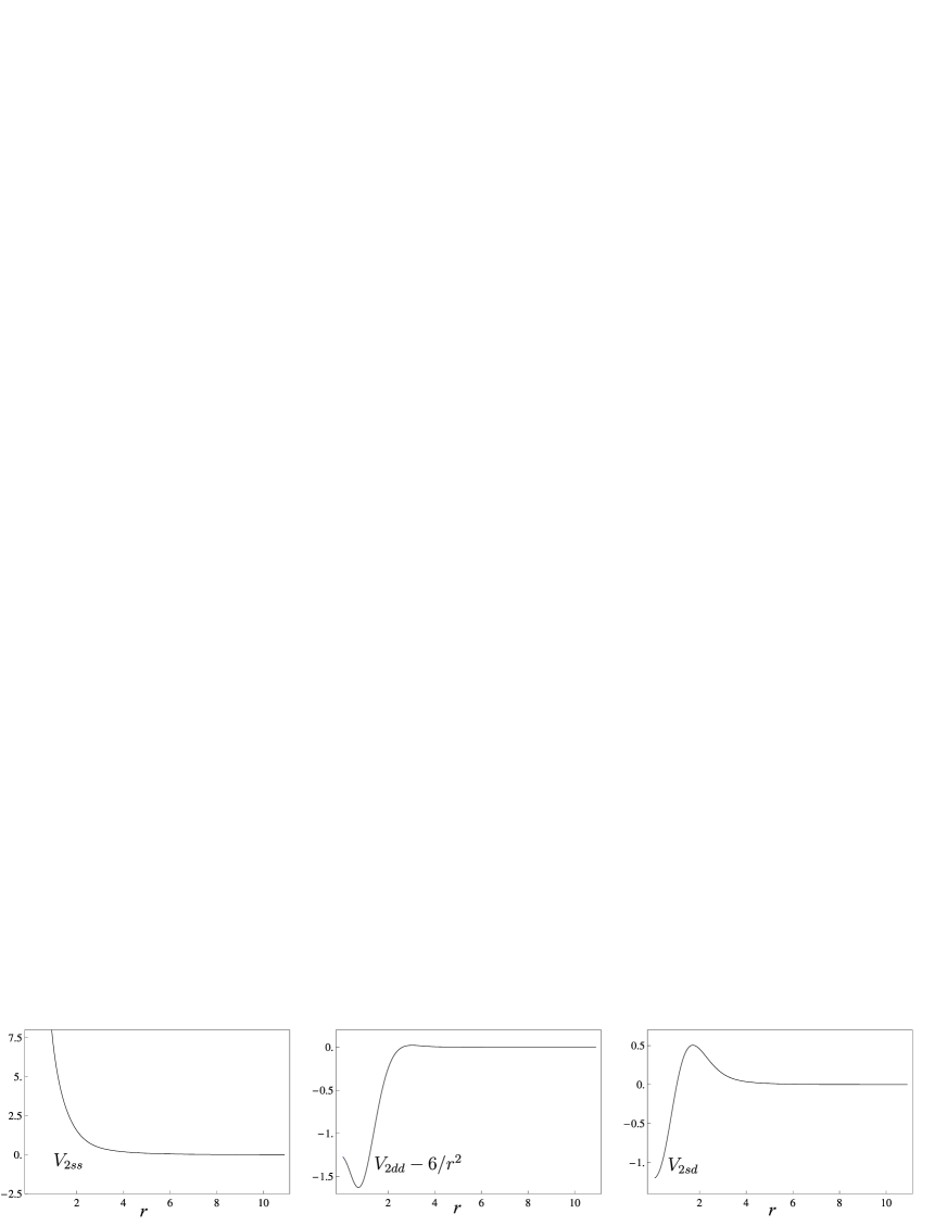
Figure 1: Entries of the exactly solvable potential matrix $V_{2}$ obtained from the uncoupled potential (75) with parameters $\kappa_{1}=0.232\,,\kappa_{2}=0.944$ by application of the eigenphase preserving transformation with $\chi=1.22$.

5 Conclusion

In this paper, we have introduced an “eigenphase preserving” two-fold SUSY transformation for the two-channel Schrödinger equation, i.e. a transformation that alters the mixing parameter between channels without modifying the eigenphase shifts. Chains of such transformations lead to coupling between channels in the scattering matrix which correspond to nontrivial $k$-dependences of the mixing angle (73). With a reasonably small number of parameters, such mixing angles are probably able to fit experimental data, in a similar way to the usual phase shift fitting used in one-channel SUSY inversion [24, 18]. Combining both techniques, we obtain a complete method of coupled-channel scattering data inversion based on SUSY transformations. As a first application of this method, we plan to invert the two-channel neutron-proton scattering data, hence improving the result of [6].

We also plan to study the following questions, raised by the present work. How do bound states transform under this eigenphase preserving transformation? How to construct a similar transformation for an arbitrary number of coupled channels? Do other forms of eigenphase preserving transformations exist? How will the presence of the Coulomb interaction modify the properties of the eigenphase preserving SUSY transformation?

Appendix A

Let us calculate asymptotics (55) using the Wronskian representation (41). This allows us to avoid manipulations with singular quantities which appear in (54) when $l_{1}=l_{2}$. It is convenient to rewrite the asymptotic behaviour of the transformation solution in the form

$$u(r\rightarrow\infty)\to\left(2Q_{\mp}-\frac{i}{\xi_{1}}\Lambda Q_{\mp}\sigma_{z}\right){\rm e}^{-i\xi_{1}\sigma_{z}}\,,\qquad Q_{\mp}=(\mathbf{1}\mp\sigma_{y})/2\,,\qquad\xi_{1}=k_{1}r,$$ (85)

where $\Lambda=\mbox{\rm diag}(\Lambda_{1},\Lambda_{2})$, $\sigma_{x}$, $\sigma_{y}$ and $\sigma_{z}$ are the Pauli matrices, and the projection matrices $Q_{\mp}$ satisfy

$$Q_{\pm}^{T}=Q_{\mp}\,,\qquad Q_{\pm}Q_{\mp}=0\,,\qquad Q_{\pm}^{2}=Q_{\pm}\,,$$ (86)

$$Q_{\pm}\sigma_{z}=\sigma_{z}Q_{\mp}\,,\qquad Q_{\pm}\sigma_{x}=\sigma_{x}Q_{\mp}.$$ (87)

Here and in what follows we will only retain terms of order $r^{-1}$ or lower. Let us first calculate the Wronskian asymptotics at large distances. Definition (26) leads to

$${\rm W}(r\to\infty)\rightarrow 4i\chi{\rm e}^{-i\xi_{1}\sigma_{z}}(\sigma_{z}\pm\sigma_{x})\left[1-\frac{(1-i)}{4\chi r}(\Lambda_{1}+\Lambda_{2})\sigma_{z}Q_{\mp}\right]{\rm e}^{i\xi_{1}^{*}\sigma_{z}}\,,$$ (88)

which can be inverted (up to $r^{-1}$) to give

$${\rm W}^{-1}(r\to\infty) \rightarrow \frac{1}{8i\chi}{\rm e}^{-i\xi^{*}_{1}\sigma_{z}}\left[1+\frac{(1-i)}{4\chi r}(\Lambda_{1}+\Lambda_{2})\sigma_{z}Q_{\mp}\right](\sigma_{z}\pm\sigma_{x}){\rm e}^{i\xi_{1}\sigma_{z}}$$ (89)

$$= \frac{1}{8i\chi}{\rm e}^{-i\xi_{1}^{*}\sigma_{z}}\left[\sigma_{z}\pm\sigma_{x}+\frac{1}{2\chi r}(\Lambda_{1}+\Lambda_{2})Q_{\pm}\right]{\rm e}^{i\xi_{1}\sigma_{z}}\,.$$ (90)

We can now calculate the two-fold superpotential up to $r^{-1}$

$$W_{2} = 4i\chi^{2}u^{*}{\rm W}^{-1}u^{T}$$ (91)

$$\to \chi\left(\frac{i}{\xi_{1}^{*}}\Lambda Q_{\pm}\sigma_{z}(\sigma_{z}\pm\sigma_{x})Q_{\pm}+\frac{1}{\chi r}(\Lambda_{1}+\Lambda_{2})Q_{\pm}-\frac{i}{\xi_{1}}Q_{\pm}(\sigma_{z}\pm\sigma_{x})\sigma_{z}Q_{\pm}\Lambda\right),$$ (92)

where (86) and (87) have been used. To further simplify this expression, we also use the decomposition ${\Lambda={\bf 1}(\Lambda_{1}+\Lambda_{2})/2+\sigma_{z}(\Lambda_{1}-\Lambda_{2})}$, which leads finally to

$$W_{2}(r\to\infty)\to\frac{1}{2r}(\Lambda_{2}-\Lambda_{1})\sigma_{z}\,.$$ (93)

This expression is valid for any $l_{1}$ and $l_{2}$; it is thus also valid for the case of coinciding partial waves.

References

References

- [1] Pupasov A M, Samsonov B F, Sparenberg J-M and Baye D 2009 Coupling between scattering channels with SUSY transformations for equal thresholds J. Phys. A: Math. Theor. 42 195303
-
[2]
Gelfand I M and Levitan B M 1951 On the determination of a
differential equation from its spectral function
Dokl. Akad. Nauk SSSR 77 557-60
Gelfand I M and Levitan B M 1951 On the determination of a differential equation from its spectral function Izvest. Akad. Nauk. SSSR Math. Series 15 309-60 - [3] Marchenko V A 1955 On reconstruction of the potential energy from phases of the scattered waves Dokl. Akad. Nauk SSSR 104 695-8
- [4] Newton R G and Jost R 1955 The construction of potentials from the S-matrix for systems of differential equations Nuovo Cimento 1 590-622
- [5] Fulton T and Newton R G 1956 Explicit non-central potentials and wave functions for given -matrices Nuovo Cimento 3 677-717
- [6] Newton R G and Fulton T 1957 Phenomenological neutron-proton potentials Phys. Rev. 107 1103-11
- [7] Kohlhoff H, Küker M, Freitag H and von Geramb H V 1993 Nucleon-nucleon potentials from inversion Phys. Scr. 48 238-44
- [8] Novikov S P, Manakov S V, Pitaevskii L P and Zakharov V E 1984 Theory of Solitons: The Inverse Scattering Method (Monographs in Contemporary Mathematics) (New York: Springer)
- [9] Ablowitz M A and Clarkson P A 1992 Solitons, Nonlinear Evolution Equations and Inverse Scattering (Cambridge: Cambridge University Press)
- [10] Levitan B M 1984 Inverse Sturm-Liouville Problems (Moscow: Nauka)
- [11] Chadan K and Sabatier P C 1989 Inverse Problems in Quantum Scattering Theory, 2nd edn. (New York: Springer)
- [12] Sukumar C V 1985 Supersymmetric quantum mechanics and the inverse scattering method J. Phys. A: Math. Gen. 18 2937-55
- [13] Baye D 1993 Phase-Equivalent Potentials for Arbitrary Modifications of the Bound Spectrum Phys. Rev. A 48 2040-7
- [14] Samsonov B F 1995 On the equivalence of the integral and the differential exact solution generation methods for the one-dimensional Schrödinger equation J. Phys. A: Math. Gen. 28 6989-98
- [15] Baye D and Sparenberg J-M 2004 Inverse scattering with supersymmetric quantum mechanics J. Phys. A: Math. Gen. 37 10223-49
- [16] Bagrov V G and Samsonov B F 1995 Darboux transformation, factorization and supersymmetry in one-dimensional quantum mechanics Theor. Math. Phys. 104 1051-60
- [17] Sparenberg J-M and Baye D 1997 Inverse Scattering with Singular Potentials: A Supersymmetric Approach Phys. Rev. C 55 2175-84
- [18] Samsonov B F and Stancu F 2003 Phase shifts effective range expansion from supersymmetric quantum mechanics Phys. Rev. C 67 054005
- [19] Amado R D, Cannata F and Dedonder J-P 1988 Coupled-channel supersymmetric quantum mechanics Phys. Rev. A 38 3797-800
- [20] Amado R D, Cannata F and Dedonder J-P 1988 Formal scattering theory approach to S-matrix relations in supersymmetric quantum mechanics Phys. Rev. Lett. 61 2901-4
- [21] Amado R D, Cannata F and Dedonder J-P 1990 Supersymmetric quantum mechanics coupled channels scattering relations Int. J. Mod. Phys. A 5 3401-15
- [22] Cannata F and Ioffe M V 1992 Solvable coupled channel problems from supersymmetric quantum mechanics Phys. Lett. B 278 399-402
- [23] Cannata F and Ioffe M V 1993 Coupled channel scattering and separation of coupled differential equations by generalized Darboux transformations J. Phys. A: Math. Gen 26 L89-92
- [24] Sparenberg J-M and Baye D 1997 Supersymmetry between phase-equivalent coupled-channel potentials Phys. Rev. Lett. 79 3802-5
- [25] Leeb H, Sofianos S A, Sparenberg J-M and Baye D 2000 Supersymmetric transformations in coupled-channel systems Phys. Rev. C 62 064003
- [26] Sparenberg J-M, Samsonov B F, Foucart F and Baye D 2006 Multichannel coupling with supersymmetric quantum mechanics and exactly-solvable model for Feshbach resonance J. Phys. A: Math. Gen. 39 L639-45
- [27] Samsonov B F, Sparenberg J-M and Baye D 2007 Supersymmetric transformations for coupled channels with threshold differences J. Phys. A: Math. Theor. 40 4225-40
- [28] Pupasov A M, Samsonov B F and Sparenberg J-M 2008 Spectral properties of non-conservative multichannel SUSY partners of the zero potential J. Phys. A: Math. Theor. 41 175209
- [29] Pupasov A M, Samsonov B F and Sparenberg J-M 2008 Exactly-solvable coupled-channel potential models of atom-atom magnetic Feshbach resonances from supersymmetric quantum mechanics Phys. Rev. A 77 012724
- [30] Sparenberg J-M, Pupasov A M, Samsonov B F and Baye D 2008 Exactly-solvable coupled-channel models from supersymmetric quantum mechanics Mod. Phys. Lett. B 22 2277-86
- [31] Samsonov B F and Pecheritsin A A 2004 Chains of Darboux transformations for the matrix Schrödinger equation J. Phys. A: Math. Gen. 37 239-50
- [32] Baye D 1987 Supersymmetry between deep and shallow nucleus-nucleus potentials Phys. Rev. Lett. 58 2738-41
- [33] Sparenberg J-M and Baye D 1996 Supersymmetry between deep and shallow optical potentials for 16O + 16O scattering Phys. Rev. C 54 1309-21
- [34] Samsonov B F and Stancu F 2002 Phase equivalent chains of Darboux transformations in scattering theory Phys. Rev. D 66 034001
- [35] Taylor J R 1972 Scattering Theory: The Quantum Theory of Nonrelativistic Collisions (New York: Wiley)
- [36] Newton R G 1982 Scattering Theory of Waves and Particles (New York: Springer)
- [37] Erdélyi A, Magnus W, Oberhettinger F and Tricomi F G 1953 Higher Transcendental Functions, Vol. 2 (New York: McGraw-Hill)
- [38] Andrianov A A, Ioffe M V and Nishnianidze D N 1995 Polynomial SUSY in Quantum Mechanics and Second Derivative Darboux Transformation Phys. Lett. A 201 103-10