Resolving photon-shortage mystery in femtosecond magnetism

Abstract

For nearly a decade, it has been a mystery why the small average number of photons absorbed per atom from an ultrashort laser pulse is able to induce a strong magnetization within a few hundred femtoseconds. Here we resolve this mystery by directly computing the number of photons per atom layer by layer as the light wave propagates inside the sample. We find that for all the 24 experiments considered here, each atom has more than one photon. The so-called photon shortage does not exist. By plotting the relative demagnetization change versus the number of photons absorbed per atom, we show that depending on the experimental condition, 0.1 photon can induce about 4% to 72% spin moment change. Our perturbation theory reveals that the demagnetization depends linearly on the amplitude of laser field. In addition, we find that the transition frequency of a sample may also play a role in magnetization processes. As far as the intensity is not zero, the intensity of the laser field only affects the matching range of the transition frequencies, but not whether the demagnetization can happen or not.

I I. introduction

The pioneering discovery by Beaurepaire et al. beaure , that a femtosecond laser pulse can demagnetize Ni on a subpicosecond time scale or femtomagnetism, has inspired enormous scientific activities both experimentally and theoretically ji ; ogasa ; zhang ; anjan ; muneaki ; bigot . The significance of this discovery is that it demonstrates a possibility for nonthermal writing in a ferromagnetic medium. One prominent example is the inverse Faraday effect, where the laser can nonthermally switch spins stanciu . This process works even better when the temperature is lowered hohlfeld01 . Its potential applications require a good understanding of the underlying excitation mechanism. In spite of extensive investigations in this field scholl ; hohlfeld00 , how the light transfers the photon energy to the system and subsequently demagnetizes the sample is still puzzling though new theoretical and experimental investigations emerge bigot . At the center of the debate is whether there are enough photons absorbed per atom (estimated at 0.01 stanciu1 ) for magnetic moment change stanciu ; stanciu1 ; koopmans00 ; koopmans01 ; koopmans02 ; dalla ; zhang02 ; woodford ; wilks01 ; atxitia ; steiauf . On the one hand, Koopmans et al. argue that the excitation density is too low to induce any substantial change in magnetization koopmans00 ; koopmans01 ; koopmans02 . If the number of photons is not enough in the first place, the excitation density must be very low. On the other hand, nearly all the experiments report the magnetization change either directly or indirectly. A strong demagnetization is incompatible with a shortage of photons. This puzzle affects our confidence in femtomagnetism hertel ; vahaplar . Therefore, resolving this apparent contradiction is of paramount importance to femtomagnetism and its future applications.

To this end, there are very few detailed investigations. Koopmans et al. koopmans04 ; koopmans02 stated that an effective photon number for demagnetization can only quench the magnetic moment of 10^-4 $\rm\mu_{B}$/atom, which is much lower than the observed demagnetization of 0.003 $\rm\mu_{B}$/atom. In 2007, Dalla et al. dalla investigated the influence of photon angular momentum on the ultrafast demagnetization in Ni. Their results excluded direct transfer of angular momentum to be relevant for the demagnetization process and showed that the photon contribution to demagnetization is less than 0.01%. This motivated them and others to search for alternative mechanisms for strong demagnetization besides the spin-orbit coupling based mechanism zhang01 . Such argument is reiterated by Stanciu et al. in Refs. stanciu ; stanciu1 . Very recently, Hertel hertel , in a viewpoint on Ref. vahaplar , claimed that the apparently simple assumption of a direct transfer of the photon spin to the magnetic system is not the solution. Majority of research merely avoid this contradiction by referring to the theoretical argument made in the early work koopmans02 and the circularly polarized experiment in nickel dalla . As we pointed out in a previous paper zhang02 , the insensitivity of magnetization change to the light polarization is not a sufficient condition to rule out the direct involvement of photons in the first place. Laser affects the spin moment change in two ways. One is that the light changes the magnetic angular momentum $m_{s}$. This is the case for the circularly polarized light. The other way is that the light changes the angular momentum $l$. This is the case for both the circularly and linearly polarized lights. If the magnetization change is not sensitive to circularly polarized lights, it only means that the $m_{s}$ channel is not effective, but it can not exclude the $l$-channel. As a result, one can not exclude the photon mechanism. A very recent theoretical investigation by Woodford woodford reinforces this concept. Nevertheless it is important to note that irrespective of underlying mechanisms, such a low photon number is unlikely to induce a substantial magnetization in a sample.

In this paper, we develop a generic scheme to compute the average photons absorbed per atom and show that for all 24 sets of experimental data considered here, each atom has more than 1 photon. For a weak laser field, we examine the relation between the relative demagnetization change and the mean photons absorbed per atom. Our results show that the small number of photons absorbed per atom can induce a strong magnetization. Moreover, the linear dependence of demagnetization change on the amplitude of laser field is consistent with our perturbation result. For the strong laser intensity, we resort to the two-level model system. We find that an effective demagnetization change occurs even with a weak laser field as far as the system is at resonance.

This paper is structured as follows. Section II presents a formal algorithm to compute the photon number in femtosecond magnetism. In Sec. III we show the relation between the relative demagnetization change and the mean photons absorbed per atom. Then we present a theoretical investigation on the demagnetization change from the perturbation theory in Sec. IV. For a strong field, results are presented in a two-level model in Sec. V. Finally, the main conclusions of our study are summarized in Sec. VI

II II. photon number in femtosecond magnetism

We start with a laser pulse propagating along the positive z axis with the field along the x axis,

$${\cal E}{{}_{x}}(\omega,\tau,z;t)=A_{0}\exp{(-t^{2}/{\tau}^{2})}\exp{\left[i\omega\left(\frac{z}{v}-t\right)\right]}$$ (1)

where $A_{0}$ is the amplitude of laser field, $\tau$ is the pulse duration, $v$ is the phase velocity, $\omega$ is the laser frequency and $t$ is the time. Since $v=c/(n+ik)$, we can rewrite the above equation as

$${\cal E}_{x}(\omega,\tau,z;t)=A_{0}\exp{(-t^{2}/{\tau}^{2})}\exp{\left[i\omega\left(\frac{nz}{c}-t\right)\right]}\exp{(-\frac{\omega k}{c}z)}$$ (2)

where $n$ and $k$ are real and imaginary parts of the index of refraction, respectively, and both are wavelength-dependent. $c$ is the speed of light.

The laser intensity $I$ for the linearly polarized light is computed from boyd

$$I(\omega,\tau,z;t)=2n\epsilon_{0}c|{\cal E}{{}_{x}}(\omega,\tau;t)|^{2}=2n\epsilon_{0}cA_{0}^{2}\exp{(-2t^{2}/{\tau}^{2})}\exp{(-\frac{2\omega k}{c}z)}$$

$$\equiv I_{0}(\omega,\tau;t)\exp{(-\frac{z}{d})}$$ (3)

where $\epsilon_{0}$ is the permittivity of free space and $I_{0}(\omega,\tau;t)$ is the laser intensity before penetrating the sample. This is the well-known Beer-Lambert law. Here $d$ is the penetration depth, defined as $d=c/2\omega k=\lambda/4\pi k$, which describes how the light intensity falls off starting from the surface of a sample. It is clear that $d$ itself is intensity-independent. Since we are interested in the pulse energy fluence ${F}(\omega,\tau,z)$, we integrate the above equation over time and find,

$${F}(\omega,\tau,z)=2nc\epsilon_{0}\int^{\infty}_{-\infty}|{\cal E}{{}_{x}}(\omega,\tau,z;t)|^{2}dt,$$ (4)

which can be simplified as

$$F(\omega,\tau,z)=2nc\epsilon_{0}A_{0}^{2}\sqrt{\frac{\pi}{2}}\tau\exp{(-\frac{z}{d})}\equiv F_{max}\exp{(-\frac{z}{d})}.$$ (5)

where $F_{max}$ is the initial laser fluence given in experiments. This is the exact expression for the laser energy fluence at depth $z$, if the pulse is a Gaussian function.

If a laser pulse of fluence $F(\omega,\tau,z)$ shines on a spot with area $A$, the total number of photons within $A$ at depth $z$ is

$$N_{photon}(\omega,z)=\frac{F_{max}A}{\hbar\omega}\exp{(-\frac{z}{d})}$$ (6)

where $\hbar\omega$ is the photon energy, and $\hbar$ is the Planck’s constant over $2\pi$. This equation reveals some crucial information: (i) $N_{photon}$ is a surface quantity; (ii) the number of atoms illuminated by these photons must be a surface quantity as well. In other words, we must compute the photon numbers provided per atom layer by layer, since the light wave propagates uniaxially. Consider an fcc structure with lattice constant $a$ and surface area $A$, the number of atoms in each layer is

$$N_{atom}=\frac{2A}{a^{2}}$$ (7)

where 2 comes from the fact that each unit cell has two atoms per layer. The mean number of photons available to each atom at different depth $z$ is

$$\Xi(z)=\frac{N_{photon}(\omega,z)}{N_{atom}}=\frac{F_{max}}{h\nu}\frac{a^{2}}{2}\exp{(-\frac{z}{d})}\equiv\Xi_{max}\exp{(-\frac{z}{d})}.\\$$ (8)

where $\Xi_{max}$ is the maximum mean number of photons provided to each atom in the top layer. This equation gives the true mean number of photons provided to each atom for demagnetization at depth $z$.

Under the low pulse energy fluence, ignoring small reflected photons, which is justified in highly absorbed metals, we estimate the photons absorbed per atom at the $j$th layer as

$$\eta_{j}=\Xi_{max}\left[\exp\left(-\frac{(j-1)a}{2d}\right)-\exp\left(-\frac{ja}{2d}\right)\right],\qquad j=1,2,3,\cdots$$ (9)

To appreciate how large $\Xi$ and $\eta_{j}$ are, in Table I we list the results from 24 different sets of experimental data increasing from top to bottom. This table is very telling. The maximum photon number $\Xi_{max}$ ranges from 1.368 to 90.430. The photon number at the penetration depth $\Xi(d)$ varies from 0.503 to 33.267. Note that since majority of samples are thinner than the penetration depth, the number of photons available to each atom exceeds 1. Here we emphasize that there are enough photons for each atom. Absorbed photon in the first layer $\eta_{1}$ ranges from 0.017 to 1.075. The mean photons absorbed per atom within the sample is less than $\eta_{1}$. Koopmans’ group koopmans01 has the smallest value of 0.017. Beaurepaire et al. beaure ’s $\eta_{1}$ value is 0.176, ten times higher than that of Koopmans’ $\eta_{1}$. Cheskis et al. cheskis00 have the largest $\eta_{1}$ value of 1.075 or roughly one photon per atom, and importantly they already found that the demagnetization is saturated. This provides a first indication that one does not need a large amount of photons to demagnetize the sample. The small number of photons absorbed does not necessarily mean that they can not induce a strong magnetization change.

III III. demagnetization change vs photons absorbed

We need to map out the connection between the magnetization change and number of the photons absorbed. We investigate the relative demagnetization changes $\Delta M/M$ which are extracted from their corresponding literatures versus the photons absorbed per atom for a weak laser intensity bigot ; beaure ; cheskis00 ; atxitia ; koopmans00 ; koopmans01 ; wilks01 . We purposely choose a weaker intensity in order to search for a one-to-one correspondence between the number of photons absorbed and the amount of magnetization change. For a strong laser, due to the saturation, such a relation will become complicated. To find some valuable information on the demagnetization mechanism associated with the number of photons, it’s necessary to estimate the mean photons absorbed per atom $\bar{\eta}$ more accurately. Based on Eq. (9), $\bar{\eta}$ is computed from

$$\bar{\eta}=\frac{1}{k}\sum_{j=1}^{k}\eta_{j}$$ (10)

where $k$ is the number of layers within the sample’s thickness. If the samples’ thickness is thinner than the penetration depth, we calculate $\bar{\eta}$ averaged within the sample’s thickness, or else within the penetration depth. The $\bar{\eta}$ itself includes the reflected and absorbed photons.

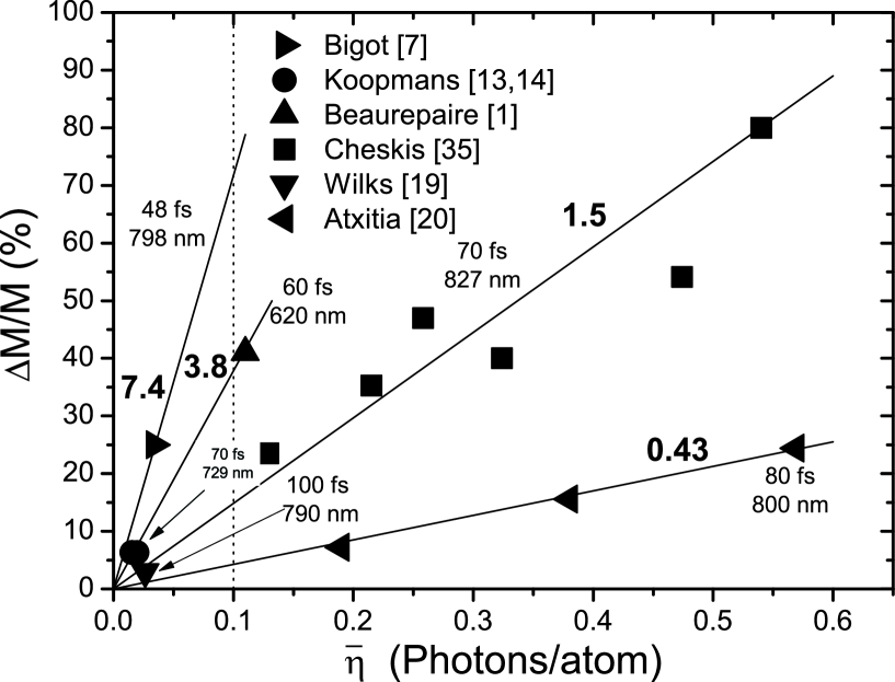
Figure 1: Dependence of the relative demagnetization changes on the average photons absorbed per atom for six different sets of experimental data. The solid lines are guides for the eye, whose slopes are shown on the lines. The laser pulse durations and the photon wavelengths are also given near their data.

Figure 1 shows $\Delta M/M$ as a function of $\bar{\eta}$. Four solid lines (guide for the eye) from top to bottom represent the results by Bigot et al. bigot , Beaurepaire et al. beaure , Cheskis et al. cheskis00 and Atxitia et al. atxitia , respectively. The corresponding results from Koopmans et al. koopmans00 ; koopmans01 and Wilks et al. wilks01 are also shown in the bottom left corner of the figure. The vertical dotted line shows that 0.1 photon can induce about 4% to 72% spin momentum change for different laser durations. This figure is very insightful. (i) The slope of these lines approximately characterizes the demagnetization ability of a laser pulse. Each solid line denotes the results obtained by an identical laser pulse which has the same pulse duration; (ii) The amplitude of laser $A_{0}$ plays a key role in the demagnetization change. For the same fluence, as predicted by Eq. (5), the smaller the pulse duration is, the bigger the laser amplitude becomes. Within the dipole approximation, the interaction between the laser and the system is dominated by the amplitude of laser. Therefore, for same $\bar{\eta}$, the amplitudes increase from bottom to top; (iii) With the same pulse duration parameter, the demagnetization change increases along with the photons absorbed per atom or the laser fluence. The solid lines with slopes of 1.5, 3.8 and 7.4 indicate that one does not need a large amount of photons to induce a substantial moment change. For Koopmans et al. koopmans00 ; koopmans01 and Wilks et al. wilks01 data, because their laser energy fluences are very small and the pulse durations are long, the demagnetization changes are much smaller, but are still consistent with the above picture.

From Fig. 1, it is obvious that the laser amplitude plays a crucial role in the demagnetization changes. However, is the laser amplitude the only deciding factor for demagnetization change? The answer is negative. In fact, using the concept of photons absorbed per atom to explain the strong demagnetization change obviously neglects two very important factors. First, it doesn’t take into account the interaction between the light and the material. Light has the energy (how strongly the field oscillates) and the frequency (how fast the field oscillates with time). $\bar{\eta}$ only takes into account the energy but not the frequency, nor the transition matrix elements between different states. Second, once the number of photons per atom becomes small, it is well known that the quasi-classical description of photons absorbed per atom for demagnetization becomes invalid. In particular, when the average number of photons provided to each atom is less than 40, the electric field behaves quantum mechanically 3 , i.e., the field oscillates strongly around its average value. The less the photons are per atom, the stronger the oscillation is. Therefore, it is necessary to reconsider this hurdle from a different perspective, and we examine this issue from the perturbation theory and two-level model, respectively.

IV IV. perturbation theory and weak intensity

In Sec. III, it reveals that the relative demagnetization change $\Delta M/M$ is proportional to the mean photons absorbed per atom $\bar{\eta}$ under a weak laser field. This allows us to treat the laser field perturbatively. The Hamiltonian of a system can be described by $H=H^{0}+H^{I}$, where $H^{0}$ is the time-independent Hamiltonian of the unperturbed system, $H^{I}=-e\vec{\mu}\cdot\vec{\cal E}(t)$ is the time-dependent perturbation. We start with the Liouville equation $i\hbar\dot{\rho}=[H,\rho]$ for the density matrix. We keep only the first order term and have

$$i\hbar\dot{\rho}^{(1)}=[H^{0},\rho^{(1)}]+[H^{I},\rho^{(0)}].$$ (11)

where $\rho^{(0)}$ and $\rho^{(1)}$ are the zeroth and first order of the density matrices, respectively. If we make an unitary transformation as $\rho^{(1)}=e^{-iH^{0}t/\hbar}Qe^{iH^{0}t/\hbar}$, and Eq. (11) can be written as

$$i\hbar\dot{Q}=e^{iH^{0}t/\hbar}[H^{I},\rho^{(0)}]e^{-iH^{0}t/\hbar}$$ (12)

We integrate this equation over time and take $\rho^{(1)}(-\infty)=0$. Then apply the eigenstate $\langle n|$ on the left and $|m\rangle$ on the right of this equation, and we can obtain

$$\rho^{(1)}_{nm}(t)=\frac{1}{i\hbar}(\rho^{(0)}_{nn}-\rho^{(0)}_{mm})e\mu_{nm}e^{-i\omega_{nm}t-\Gamma t}\int^{t}_{-\infty}dt^{\prime}{\cal E}(t^{\prime})e^{i\omega_{nm}t^{\prime}-\Gamma t^{\prime}}$$ (13)

where $\omega_{nm}=(E_{n}-E_{m})/{\hbar}$, $\mu_{nm}$ the transition matrix elements, and $\Gamma$ the damping factor. Theoretically, the demagnetization change is involved in the time-dependent density matrix $\rho^{(1)}_{nm}(t)$ through $M_{z}^{(1)}(t)=Tr[S_{z}\rho^{(1)}(t)]$, where $S_{z}$ is the spin matrix. By investigating the density matrix, we can reveal some crucial details of the demagnetization. Next we discuss two typical cases.

Case 1, Continuum wave laser. Consider a periodical field perturbation $H^{I}=-e\mu A_{0}e^{-i\omega t}$, the density matrix becomes

$$\rho^{1}_{nm}(t)=\frac{e\mu_{nm}}{i\hbar}(\rho^{(0)}_{nn}-\rho^{(0)}_{mm})A_{0}e^{-2\Gamma t}\frac{(\Delta\omega\sin{\omega t}-\Gamma\cos{\omega t})+(\Delta\omega\cos{\omega t}+\Gamma\sin{\omega}t)i}{\Delta\omega^{2}+\Gamma^{2}}$$ (14)

where $\Delta\omega=\omega-\omega_{nm}$. Note that its frequency dependence is exactly same even if we treat photons quantum mechanically. It shows that the density matrix $\rho^{(1)}_{nm}(t)$ not only depends on the amplitude of laser field $A_{0}$ which is consistent with the conclusion obtained from Fig. 1, but also depends on the resonance term $(\frac{1}{\Delta\omega^{2}+\Gamma^{2}})$. Since the spin moment change is directly proportional to $\rho^{(1)}_{nm}(t)$, this predicts that the magnetic moment change will depend linearly on the amplitude of laser field in the weak field limit. On the other hand, the resonance term demonstrates that even for the exactly same laser amplitude, the transition or the magnetic change can be very different for different frequencies. This has been largely ignored in the literature.

Case 2, Pulse laser. We assume that laser field has a form $H^{I}=-e\mu A_{0}e^{-t^{2}/\tau^{2}}e^{-i\omega t}$. Eq. (13) becomes

$$\rho^{(1)}_{nm}(t) =\frac{e\mu_{nm}}{i\hbar}(\rho^{(0)}_{nn}-\rho^{(0)}_{mm})e^{-i\omega_{nm}t-\Gamma t}A_{0}\int^{t}_{-\infty}dt^{\prime}e^{-t^{\prime 2}/\tau^{2}}e^{-i\Delta\omega t^{\prime}-\Gamma t^{\prime}}$$ (15)

$$\equiv\frac{e\mu_{nm}}{i\hbar}(\rho^{(0)}_{nn}-\rho^{(0)}_{mm})e^{-i\omega_{nm}t-\Gamma t}R(t)$$

where $R(t)$ is defined as the module of response function. To get some insightful information about the perturbation of laser field, we choose $\rm\tau=12$ $\rm fs$, and $A_{0}=0.05$ V/Å, and integrate the response function numerically.

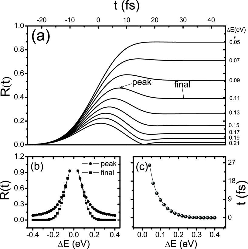
Figure 2: (a) The module of response function $R(t)$ as a function of time at different $\Delta E$. (b) The dependence of the peak and final values on $\Delta E$. (c) The time needed to reach the peak as a function of $\Delta E$.

Figure 2(a) shows the module of response function $R(t)$ as a function of time for twelve different energy detuning $\Delta E$ ($\hbar\Delta\omega$) from 0.05 to 0.21 eV. We can see that as time goes by, $R(t)$ first increases to a peak value, and then settles down to its final value. Importantly the peak values of $R(t)$ vary a lot for different $\Delta E$ even with the same laser field amplitude. The biggest one is about 0.9 ($\Delta E$ = 0.05 eV) and the smallest one is about 0.07 ($\Delta E$ = 0.15 eV). Their difference is over an order of magnitude. It demonstrates that the transition probability or spin momentum change can be very large when $\Delta E$ becomes very small or the system is excited resonantly, even if the field intensity is weak.

Figure 2(b) compares the peak and final values of $R(t)$ as a function of $\Delta E$. The final $R(t)$ values decrease more quickly with $\Delta E$ than that of peak ones. The maximum difference is 0.16 at $\Delta E=0.22$ eV, and the minimum difference is 0.09 at $\Delta E=0.4$ eV. When $\Delta E$ reaches 0.07 eV, the peak and final values are almost same. It implies that regardless of the amplitude of laser field the transition from one state to another state is finished when $\Delta E$ goes to zero. Figure 2(c) shows the time needed reaching the peak value as a function of $\Delta E$. This indicates that the peak time is reduced as $\Delta E$ becomes larger. All the above results are obtained within a weak field limit. Once the laser field becomes strong, the first order perturbation becomes invalid. Under this situation, we resort to a two-level model system.

V V. two-level model and strong intensity

The two-level model has been extensively used in atoms allen ; lesovik , semiconductors du ; kunikeev ; badescu and ferromagnetic materials 5 . For a system excited by a laser, the two-level model can give us a quantitative understanding of the spin transition. Here we directly quote the Eq. (7) of Ref. 5 in our previous work about the spin change $\Delta S_{z}$ for a transition from state $|a\rangle$ to state $|b\rangle$

$$\Delta S_{z}=\aleph_{ab}(t;\omega)(\langle b|s_{z}|b\rangle-\langle a|s_{z}|a\rangle)$$ (16)

where $t$ is time, and $\omega$ is laser frequency. $\aleph_{ab}(t;\omega)$, the probability amplitude of finding the system at time $t$ in state $|b\rangle$, is equal to

$$\aleph_{ab}(t;\omega)=\frac{|W_{ab}|^{2}}{|W_{ab}|^{2}+\hbar^{2}(\omega-\omega_{ba})^{2}}\sin^{2}\left[\sqrt{\frac{|W_{ab}|^{2}}{\hbar^{2}}+(\omega-\omega_{ba})^{2}}\frac{t}{2}\right]$$ (17)

where $W_{ab}=\mu_{ab}A_{0}$. The transition matrix elements $\mu_{ab}$ can be obtained by calculating the corresponding momentum operator $\vec{p}_{ab}$ from the $ab$ $initio$ calculation 6 ; 7 ; 8 .

The probability $\aleph_{ab}(t;\omega)$ is an oscillatory function of time; for certain values of $t$, $\aleph_{ab}(t;\omega)=0$, meaning that the system returns to the initial state $|a\rangle$. At the same time it also reveals fast oscillation expressed by the latter term of Eq. (17). If $|W_{ab}|$ is large enough, the value of $\aleph_{ab}(t;\omega)$ or $\Delta S_{z}$ can be very large. For the off-resonance excitation, the laser field amplitude $A_{0}$ controls the demagnetization change entirely. This happens in semiconductors. For the resonance excitation, or $\omega=\omega_{ba}$, regardless of how weak the perturbation is, the field can cause the system to transit from state $|a\rangle$ to state $|b\rangle$ 10 . Importantly, the field intensity only affects the time needed for the system to transit from $|a\rangle$ to $|b\rangle$, not whether a transition can occur or not. The smaller the field intensity is, the longer the time it takes.

For a ferromagnetic metal like nickel, the chance that the transition frequency $\omega_{ba}$ matches that of the laser field is very high zhang001 . This explains the observed demagnetization in those experiments, in spite of a relatively weak laser electric field. Figure 3 shows the detailed dependence of the spin change on the laser electric field. For a weak laser field intensity with 0.001 V/Å, the spin change is possible as far as $\omega_{ba}$ matches $\omega$. This demonstrates that the strong demagnetization change is achievable in experiments even if the laser field intensity is very weak. If the laser field becomes larger, the range of matching frequency becomes broad (see Fig. 3). In semiconductors, Pavlov et al. 11 showed that increasing temperature reduces the GaAs band gap. This may be a test case for our theory.

VI VI. conclusion

We have clarified a long-standing conceptual puzzle of the photon shortage in femtosecond magnetism by comparing the relative demagnetization change versus the mean photons absorbed per atom. In the weak laser field, it increases along with the mean photons absorbed per atom $\bar{\eta}$, which is consistent with the perturbation theory. Importantly, the results show that few photons absorbed per atom can induce considerable spin moment changes. The spin moment can be reduced at resonance even if the field is weak. Our findings overcome a big hurdle in ferromagnetism and should inspire new experimental and theoretical investigations into the role of photons and their interactions with electrons in the magnetization change.

VII acknowledgments

We would like to thank B. Koopmans (TUE, Netherlands) for valuable communication. We appreciate Markus Münzenberg (Göttingen University) for numerous discussions and for their experimental results before publication of their preprint Ref. atxitia . This work was supported by the U. S. Department of Energy under Contract No. DE-FG02-06ER46304, U.S. Army Research Office under Contract No. W911NF-04-1-0383, the NSFC under No. 10804038, and was also supported by a Promising Scholars grant from Indiana State University. We acknowledge part of the work as done on Indiana State University’s high-performance computers. This research used resources of the National Energy Research Scientific Computing Center at Lawrence Berkeley National Laboratory, which is supported by the Office of Science of the U.S. Department of Energy under Contract No. DE-AC02-05CH11231. Initial studies used resources of the Argonne Leadership Computing Facility at Argonne National Laboratory, which is supported by the Office of Science of the U.S. Department of Energy under Contract No. DE-AC02-06CH11357.

^∗gpzhang@indstate.edu

Table 1: The calculated number of photons per atom in Ni. $\Xi_{max}$ is the maximum photon number per atom. $d$ is the optical penetration depth. $\Xi(d)$ is the photon number at $d$. $\eta_{1}$ is the photons absorbed per atom in the first top layer. The other parameters are taken from the literature. $n$ and $k$ are real and imaginary parts of the index of refraction palik , respectively.

No.	$F$	$\lambda$	$n+ik$	$d$	$\Xi_{max}$	$\Xi(d)$	$\eta_{1}$	Ref.
	($\rm mJ/cm^{2}$)	(nm)		(nm)
1	0.6	729	2.28+4.18$i$	13.93	1.368	0.503	0.017	koopmans01
2	0.76	729	2.28+4.18$i$	13.93	1.741	0.641	0.022	koopmans00
3	1.4	790	2.46+4.35$i$	14.45	3.457	1.272	0.042	wilks01
4	1.45	798	2.476+4.375$i$	14.52	3.617	1.331	0.044	bigot
5	1.8	800	2.48+4.38$i$	14.45	4.501	1.656	0.055	regens00
6	2.04	729	2.28+4.18$i$	13.93	4.644	1.708	0.058	koopmans00
7	2.0	785	2.45+4.34$i$	14.50	4.908	1.805	0.059	dalla
8	2.0	800	2.48+4.38$i$	14.45	5.001	1.840	0.061	wilks00
9	2.5	800	2.48+4.38$i$	14.45	6.252	2.300	0.076	hohlfeld00
10	2.83	800	2.48+4.38$i$	14.45	7.075	2.603	0.086	melnikov00
11	3.5	800	2.48+4.38$i$	14.45	8.752	3.220	0.106	hohlfeld00
12	4.4	800	2.48+4.38$i$	14.45	11.003	4.048	0.133	hohlfeld00
13	5.3	800	2.48+4.38$i$	14.45	13.254	4.876	0.161	hohlfeld00
14	7.0	620	1.93+3.65$i$	13.53	13.566	4.991	0.176	beaure ; bigot01
15	6.0	800	2.48+4.38$i$	14.45	15.004	5.520	0.182	hohlfeld
16	8.0	620	1.93+3.65$i$	13.52	15.504	5.704	0.201	bigot01
17	7.1	800	2.48+4.38$i$	14.45	17.755	6.532	0.215	regens00
18	12.0	800	2.48+4.38$i$	14.45	30.008	11.039	0.364	gudde
19	12.73	827	2.53+4.47$i$	14.73	32.897	12.102	0.391	scholl
20	13	827	2.53+4.47$i$	14.73	33.588	12.356	0.399	rhie
21	13.3	827	2.48+4.38$i$	14.73	34.363	12.642	0.409	cheskis00
22	15.72	800	2.48+4.38$i$	14.45	39.308	14.461	0.476	conrad00
23	20	800	2.48+4.38$i$	14.45	50.014	18.400	0.606	georg00
24	35	827	2.13+4.17$i$	14.73	90.430	33.267	1.075	cheskis00

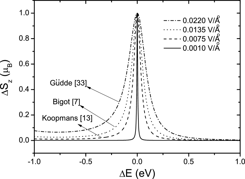
Figure 3: Amplitude of spin momentum change as a function of the detuning $\Delta E=\hbar(\omega-\omega_{ba})$ for three groups at different laser electric fields. The amplitude of laser field is deduced from the experimental laser fluence based on the Eq. (5). All the curves are shifted to zero at resonance.

References

- (1) E. Beaurepaire, J.-C. Merle, A. Daunois, and J.-Y. Bigot, Phys. Rev. Lett. 76, 4250 (1996).
- (2) J.-W. Kim, K.-D. Lee, J.-W. Jeong, and S.-C. Shin, Appl. Phys. Lett. 94, 192506 (2009).
- (3) T. Ogasawara, N. Iwata, Y. Murakami, H. Okamoto, and Y. Tokura, Appl. Phys. Lett. 94, 162507 (2009).
- (4) G. P. Zhang, W. Hübner, G. Lefkidis, Y. Bai, and T. F. George, Nature Phys. 5, 499 (2009).
- (5) A. Barman and S. Barman, Phys. Rev. B 79, 144415 (2009).
- (6) M. Hase, Y. Miyamoto, and J. J. Tominaga, Phys. Rev. B 79, 174112 (2009).
- (7) J.-Y. Bigot, M. Vomir, and E. Beaurepaire, Nature Phys. 5, 515 (2009).
- (8) C. D. Stanciu, F. Hansteen, A. V. Kimel, A. Kirilyuk, A. Tsukamoto, A. Itoh, and Th. Rasing Phys. Rev. Lett. 99, 047601 (2007).
- (9) J. Hohlfeld, C. D. Stanciu, and A. Rebei, Appl. Phys. Lett. 94, 152504 (2009).
- (10) A. Scholl, L. Baumgarten, R. Jacquemin, and W. Eberhardt, Phys. Rev. Lett. 79, 5146 (1997).
- (11) J. Hohlfeld, E. Matthias, R. Knorren, and K. H. Bennemann, Phys. Rev. Lett. 78, 4861 (1997).
- (12) C. D. Stanciu, Laser-Induced Femtosecond Magnetic Recording (Ph.D. Thesis, Nijmegen, The Netherlands, 2008).
- (13) B. Koopmans, M. van Kampen, J. T. Kohlhepp, and W. J. M. de Jonge, Phys. Rev. Lett. 85, 844 (2000).
- (14) B. Koopmans, M. van Kampen, J. T. Kohlhepp, and W. J. M. de Jonge, J. Appl. Phys. 87, 5070 (2000).
- (15) B. Koopmans, M. van Kampen, and W. J. M. de Jonge, J. Phys.: Condens. Matter 15, S723 (2003).
- (16) F. Dalla Longa, J. T. Kohlhepp, W. J. M. de Jonge, and B. Koopmans, Phys. Rev. B 75, 224431 (2007).
- (17) G. P. Zhang and T. F. George, Phys. Rev. B 78, 052407 (2008).
- (18) S. R. Woodford, Phys. Rev. B 79, 212412 (2009).
- (19) R. Wilks, R. J. Hicken, M. Ali, B. J. Hickey, J. D. R Buchanan, A. T. G. Pym, and B. K. Tanner, J. Appl. Phys. 95, 7441 (2004).
- (20) U. Atxitia, O. Chubykalo-Fesenko, J. Walowski, A. Mann, and M. Münzenberg, arXiv:0904.4399v1 [cond-mat.mtrl-sci].
- (21) D. Steiauf and M. Fähnle, Phys. Rev. B 79, 140401(R) (2009).
- (22) R. Hertel, Physics 2, 73 (2009).
- (23) K. Vahaplar, A. M. Kalashnikova, A. V. Kimel, D. Hinzke, U. Nowak, R. Chantrell, A. Tsukamoto, A. Itoh, A. Kirilyuk, and Th. Rasing, Phys. Rev. Lett. 103, 117201 (2009).
- (24) B. Hillebrands and K. Ounadjela (eds.), Spin Dynamics in Confined Magnetic Structures (Spinger-Verlag, Berlin Heidelberg, 2003).
- (25) G. P. Zhang and W. Hübner, Phys. Rev. Lett. 85, 3025 (2000).
- (26) R. W. Boyd, Nonlinear Optics (Academic Press, Boston, 1992).
- (27) E. D. Palik, Handbook of Optical Constants of Solids (Academic Press, San Diego, 1998).
- (28) H. Regensburger, R. Vollmer, and J. Kirschner, Phys. Rev. B 61, 14716 (2000).
- (29) R. Wilks, N. D. Hughes, and R. J. Hicken, J. Phys.: Condens. Matter 15, 5129 (2003).
- (30) A. V. Melnikov, J. Güdde, and E. Matthias, Appl. Phys. B 74, 735 (2002).
- (31) J.-Y. Bigot, C. R. Acad. Sci. Paris 2, 1483 (2001).
- (32) J. Hohlfeld, J. Güdde, U. Conrad, O. Dühr, G. Korn, and E. Matthias, Appl. Phys. B 68, 505 (1999).
- (33) J. Güdde, U. Conrad, V. Jähnke, J. Hohlfeld, and E. Matthias, Phys. Rev. B 59, R6608 (1999).
- (34) H.-S. Rhie, H. A. Dürr, and W. Eberhardt, Phys. Rev. Lett. 90, 247201 (2003).
- (35) D. Cheskis, A. Porat, L. Szapiro, O. Potashnik, and S. Bar-Ad, Phys. Rev. B 72, 014437 (2005).
- (36) U. Conrad, J. Güdde, V. Jähnke, and E. Mattias, Appl. Phys. B 68, 511 (2005).
- (37) G. M. Müller, G. Eilers, Z. Wang, M. Scherff, R. Ji, K. Nielsch, C. A. Ross and M. Münzenberg, N. J. Phys. 10, 123004 (2008).
- (38) R. Loudon, The Quantum Theory of Light, page 153 (Oxford University Press, London, 1973).
- (39) L. Allen and J. H. Eberly, Optical Resonance and Two-Level Atoms (Dover Publications, New York, 1987).
- (40) G. B. Lesovik, A. V. Lebedev, and A. O. Imambekov, JETP Lett. 75, 474 (2002).
- (41) S. Du, J. Wen, M. H. Rubin, and G. Y. Yin, Phys. Rev. Lett. 98, 053601 (2007).
- (42) S. D. Kunikeev and D. A. Lidar, Phys. Rev. B 77, 045320 (2008).
- (43) S. C. Badescu and T. L. Reinecke, Phys. Rev. B 75, 041309(R) (2007).
- (44) G. P. Zhang, Phys. Rev. Lett. 101, 187203 (2008).
- (45) S. Sharma, J. K. Dewhurst, and C. Ambrosch-Draxl, Phys. Rev. B 67, 165332 (2003).
- (46) C. Ambrosch-Draxl and J. O. Sofo, Comp. Phys. Comm. 175, 1 (2006).
- (47) G. P. Zhang, Y. Bai, and T. F. George, Phys. Rev. B 80, 214415 (2009).
- (48) C. Cohen-Tannoudji, B. Diu, and F. Laloë, Quantum Mechanics, page 1340 (Hermann Press, Paris, 1973).
- (49) T. Hartenstein, G. Lefkidis, W. Hübner, G. P. Zhang, and Y. Bai, J. Appl. Phys. 105, 07D305 (2009).
- (50) V. V. Pavlov, A. M. Kalashnikova, R. V. Pisarev, I. Sänger, D. R. Yakovlev, and M. Bayer, Phys. Rev. Lett. 94, 157404 (2005).