Modeling Stop-and-Go Waves in Pedestrian Dynamics

Abstract

Several spatially continuous pedestrian dynamics models have been validated against empirical data. We try to reproduce the experimental fundamental diagram (velocity versus density) with simulations. In addition to this quantitative criterion, we tried to reproduce stop-and-go waves as a qualitative criterion. Stop-and-go waves are a characteristic phenomenon for the single file movement. Only one of three investigated models satisfies both criteria.

1 Introduction

The applications of pedestrians’ dynamics range from the safety of large events to the planning of towns with a view to pedestrian comfort. Because of the computational effort involved with an experimental analysis of the complex collective system of pedestrians’ behavior, computer simulations are run. Models continuous in space are one possibility to describe this complex collective system.

In developing a model, we prefer to start with the simplest case: single lane movement. If the model is able to reproduce reality quantitatively and qualitatively for that simple case, it is a good candidate for adaption to complex two-dimensional conditions.

Also in single file movement pedestrians interact in many ways and not all factors, which have an effect on their behavior, are known. Therefore, we follow three different modeling approaches in this work. All of them underlie diverse concepts in the simulation of human behavior.

This study is a continuation and enlargement of the validation introduced in [7]. For validation, we introduce two criteria: On the one hand, the relation between velocity and density has to be described correctly. This requirement is fulfilled, if the modeled data reproduce the fundamental diagram. On the other hand, we are aiming to reproduce the appearance of collective effects. A characteristic effect for the single file movement are stop-and-go waves as they are observed in experiments [5]. We obtained all empirical data from several experiments of the single file movement. There a corridor with circular guiding was built, so that it possessed periodic boundary conditions. The density was varied by increasing the number of the involved pedestrians. For more information about the experimental set-up, see [5],[6].

2 Spatially Continuous Models

The first two models investigated are force based and the dynamics are given by the following system of coupled differential equations

$$m_{i}\frac{d\,v_{i}}{d\,t}=F_{i}\quad\mbox{with}\quad F_{i}=F_{i}^{drv}+F_{i}^{rep}\quad\mbox{and}\quad\frac{d\,x_{i}}{d\,t}=v_{i}$$ (1)

where $F_{i}$ is the force acting on pedestrian $i$. The mass is denoted by $m_{i}$, the velocity by $v_{i}$ and the current position by $x_{i}$. This approach derives from sociology [4]. Here psychological forces define the movement of humans through their living space. This approach is transferred to pedestrians dynamics and so $F_{i}$ is split to a repulsive force $F_{i}^{rep}$ and a driven force $F_{i}^{drv}$. In our case the driving force is defined as

$$F_{i}^{drv}=\frac{v_{i}^{0}-v_{i}}{\tau},$$ (2)

where $v_{i}^{0}$ is the desired velocity of a pedestrian and $\tau$ their reaction time.

The other model is event driven. A pedestrian can be in different states. A change between these states is called event. The calculation of the velocity of each pedestrian is straightforward and depends on these states.

2.1 Social Force Model

The first spatially continuous model was developed by Helbing and Molnár [3] and has often been modified. According to [2] the repulsive force for pedestrian $i$ is defined by

$$F_{i}^{rep}(t)=\sum_{j\neq i}f_{ij}(x_{i},x_{j})+\xi_{i}(t)\quad\mbox{with}\quad f_{ij}(x_{i},x_{j})=-\partial_{x}A(\Delta\,x_{i,j}-D)^{-B},$$ (3)

with $A=0.2,B=2,D=1\,[m],\tau=0.2\,[s]$ and $\Delta\,x_{i,j}$ is the distance between pedestrians $i$ and $j$. The fluctuation parameter $\xi_{i}(t)$ represents the noise of the system. In two-dimensional scenes, this parameter is used to create jammed states and lane formations [2]. In this study, we are predominantly interested in the modeled relation between velocity and density for single file movement. Therefore the fluctuation parameter has no influence and is ignored.

First tests of this model indicated that the forces are too strong, leading to unrealistically high velocities. Due to this it is necessary to limit the velocity to $v_{max}$, as it is done in [3]

$$v_{i}(t)=\left\{\begin{array}[]{cl}v_{i}(t),&\mbox{\quad if }|v_{i}(t)|\leq v_{max}\\ v_{max},&\mbox{\quad otherwise}\end{array}\right.\enspace.$$ (4)

In our simulation we set $v_{max}=1.34\,[\frac{m}{s}]$.

2.2 Model with Foresight

In this model pedestrians possess a degree of foresight, in addition to the current state of a pedestrian at time step $t$. This approach considers an extrapolation of the velocity to time step $t+s$. For it [8] employs the linear relation between the velocity and the distance of a pedestrian $i$ to the one in front $\Delta x_{i,i+1}(t)$.

$$v_{i}(t)=a\,\Delta x_{i,i+1}(t)-b$$ (5)

For $a=0.94\,[\frac{m}{s}]$ and $b=0.34\,[\frac{1}{s}]$ this reproduces the empirical data. So with (5) $v_{i}(t+s)$ can be calculated from $\Delta x_{i,i+1}(t+s)$ which itself is a result of the extrapolation of the current state

$$\Delta x_{i,i+1}(t)+\Delta v(t)\,s=\Delta x_{i,i+1}(t+s)$$ (6)

with $\Delta v(t)=v_{i+1}(t)\,s-v_{i}(t)\,s$. Finally, the repulsive force is defined as

$$F_{i}^{rep}(t)=-\frac{v_{i}^{0}-v_{i}(t+s)}{\tau}\enspace.$$ (7)

Obviously the impact of the desired velocity $v_{i}^{0}$ in the driven force is negated by the one in the repulsive term. After some simulation time, the system reaches an equilibrium in which all pedestrians walk with the same velocity. In order to spread the values and keep the right relation between velocity and density, we added a fluctuation parameter $\zeta_{i}(t)$. $\zeta_{i}(t)$ uniformly distributed in the interval $[-20,20]$ reproduced the scatter observed in the empirical data.

2.3 Adaptive Velocity Model

In this model pedestrians are treated as hard bodies with a diameter $d_{i}$ [1]. The diameter depends linearly on the current velocity and is equal to the step length $st$ in addition to the safety distance $\beta$

$$d_{i}(t)=e+f\,v_{i}(t)=st_{i}(t)+\beta_{i}(t)\enspace.$$ (8)

Based on [9] the step length is a linear function of the current velocity with following parameters:

$$st_{i}(t)=0.235\,[m]+0.302\,[s]\,v_{i}(t)\enspace.$$ (9)

$e$ and $f$ can be specified through empirical data and the inverse relation of (5). Here $e$ is the required space for a stationary pedestrian and $f$ affects the velocity term. For $e=0.36\,[m]$ and $f=1.06\,[s]$ the last equations (8) and (9) can be summarized to

$$\beta_{i}(t)=d_{i}(t)-st_{i}(t)=0.125\,[m]+0.758\,[s]\,v_{i}(t)\enspace.$$ (10)

By solving the differential equation

$$\frac{dv}{dt}=F^{drv}=\frac{v^{0}-v(t)}{\tau}\quad\Rightarrow\quad v(t)=v^{0}+c\,\exp\left(-\frac{t}{\tau}\right),\mbox{for }c\in\bbbr,$$ (11)

the velocity function is obtained. This is shown in Fig. 1 together with the parameters of the pedestrians’ movement.

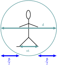
(a) Demonstration of the parameters $d,st$ and $\beta$

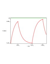
(b) Conception of the adaptive velocity

Figure 1: Left: connection between the required space $d$, the step length $st$ and the safety distance $\beta$. Right: The adaptive velocity with acceleration until $t_{dec1}$, than deceleration until $t_{acc1}$, again acceleration until $t_{dec2}$ and so on.

A pedestrian is accelerating to their desired velocity $v_{i}^{0}$ until the distance to the pedestrian in front is smaller than the safety distance. From this time on, he/she is decelerating until the distance is larger than the safety distance and so on. Via $\Delta x_{i,i+1},d_{i}$ and $\beta_{i}$ those events could be defined: deceleration (12) and acceleration (13).

To ensure good performance for high densities, no events are explicitly calculated. But in each time step, it is checked whether an event has taken place and $t_{dec},t_{acc}$ or $t_{coll}$ are set to $t$ accordingly. The time step, $\Delta t$, of $0.05$ seconds is chosen, so that a reaction time is automatically included. The discrete time step could lead to configurations where overlapping occurs. To guarantee volume exclusion, case (14) is included, in which the pedestrians are too close to each other and have to stop.

$$t = t_{dec},\quad\mbox{if: }\quad\Delta x_{i,i+1}-0.5*\left(d_{i}(t)+d_{i+1}(t)\right)\leq 0$$ (12)

$$t = t_{acc},\quad\mbox{if: }\quad\Delta x_{i,i+1}-0.5*\left(d_{i}(t)+d_{i+1}(t)\right)>0$$ (13)

$$t = t_{coll},\quad\mbox{if: }\quad\Delta x_{i,i+1}-0.5*\left(d_{i}(t)+d_{i+1}(t)\right)\leq-\beta_{i}(t)$$ (14)

3 Validation with Empirical Data

For the comparison of the modeled and experimental data, it is important to use the same method of measurement. [5] shows that the results from different measurement methods vary considerably. The velocity $v_{i}$ is calculated by the entrance and exit times $t_{i}^{in}$ and $t_{i}^{out}$ to two meter section.

$$v_{i} = \frac{2\,[m]}{(t_{i}^{out}-t_{i}^{in})[s]}.$$ (15)

To avoid discrete values of the density leading to a large scatter, we define the density by

$$\rho(t) = \frac{\sum_{i=1}^{N}\Theta_{i}(t)}{2\,m},$$ (16)

where $\Theta_{i}(t)$ gives the fraction to which the space between pedestrian $i$ and $i+1$ is inside the measured section, see [6]. $\rho_{i}$ is the mean value of all $\rho(t)$, where $t$ is in the interval $[t_{i}^{in},t_{i}^{out}]$. We use the same method of measurement for the modeled and empirical data. The fundamental diagrams are displayed in Fig. 2, where $N$ is the number of the pedestrians.

(a) Social force model

(b) Model with foresight

(c) Adaptive velocity model

(d) Empirical data

Figure 2: Validation of the modeled fundamental diagram with the empirical data (down right) for the single file movement.

The velocities of the social force model are independent of the systems density and nearly equal to the desired velocity $v_{i}=v_{i}^{0}\sim 1.24\,[\frac{m}{s}]$. Additionally we observe a backward movement of the pedestrians and pair formation. Because of these unrealistic phenomena are not observed in the other models, we suggest that this is caused by the combination of long-range forces and periodic boundary conditions.

In contrast, the model with foresight results in a fundamental diagram in good agreement with the empirical one. Through the fluctuation parameter, the values of the velocities and densities vary as in the experimental data.

We are satisfied with the results of the adaptive velocity model. For reducing computing time, we also tested a linear adaptive velocity function, leading to a $70\%$ decrease in computing time for $10000$ pedestrians. The fundamental diagram for this linear adaptive velocity function is not shown, but also reproduces the empirical one.

4 Reproduction of Stop-and-Go Waves

During the experiments of the single file movement, we observed stop-and-go waves at densities higher than two pedestrians per meter, see Fig. 5 in [5]. Therefore, we compare the experimental trajectories with the modeled ones for global densities of one, two and three persons per meter. The results are shown in Fig.3. Since the social force model is not able to satisfy the criterion for the right relation between velocity and density, we omit this model in this section. Figure 3 shows the trajectories for global average densities of one, two and three persons per meter. From left to right the data of the model with foresight, the adaptive velocity model and the experiment are shown.

In the experimental data, it is clearly visible that the trajectories get unsteadier with increasing density. At a density of one person per meter pedestrians stop for the first time. So a jam is generated. At a density of two persons per meter stop-and-go waves pass through the whole measurement range. At densities greater than three persons per meter pedestrians can hardly move forward.

For the extraction of the empirical trajectories, the pedestrians’ heads were marked and tracked. Sometimes, there is a backward movement in the empirical trajectories caused by self-dynamic of the pedestrians’ heads. This dynamic is not modeled and so the other trajectories have no backward movement. This has to be accounted for in the comparison.

By adding the fluctuation parameter $\zeta_{i}(t)\in[-20,20]$ to the model with foresight a good agreement with experiment is obtained for densities of one and two persons per meter. The irregularities caused by this parameter are equal to the irregularities of the pedestrians dynamic. Nevertheless, this does not suffice for stopping so that stop-and-go waves appear, Fig.3(d) and Fig.3(g).

(a) Model with foresight

(b) Adaptive velocity model

(c) Experimental data

(d) Model with foresight

(e) Adaptive velocity model

(f) Experimental data

(g) Model with foresight

(h) Adaptive velocity model

(i) Experimental data

Figure 3: Comparison of modeled and empirical trajectories for the single lane movement. The global density of the system is one, two or three persons per meter (from top to bottom).

With the adaptive velocity model stop-and-go waves already arise at a density of one pedestrian per meter, something that is not seen in experimental data. However, this model characterizes higher densities well. So in comparison with Fig. 3(h) and Fig. 3(i) the stopping-phase of the modeled data seems to last for the same time as in the empirical data. But there are clearly differences in the acceleration phase, the adaptive velocity models acceleration is much lower than seen in experiment.

Finally other studies of stop-and-go waves have to be carried out. The occurrence of this phenomena has to be clearly understood for further model modifications. Therefore it is necessarry to measure e. g. the size of the stop-and-go wave at a fixed position. Unfortunately it is not possible to measure over a time interval, because the empirical trajectories are only available in a specific range of 4 meters.

5 Conclusion

The well-known and often used social force model is unable to reproduce the fundamental diagram. The model with foresight provides a good quantitative reproduction of the fundamental diagram. However, it has to be modified further, so that stop-and-go waves could be generated as well. The model with adaptive velocities follows a simple and effective event driven approach. With the included reaction time, it is possible to create stop-and-go waves without unrealistic phenomena, like overlapping or interpenetrating pedestrians.

All models are implemented in C and run on a simple PC. They were also tested for their computing time in case of large system with upto 10000 pedestrians. The social force model offers a complexity level of $\mathcal{O}(N^{2})$, whereas the other models only have a level of $\mathcal{O}(N)$. For this reason the social force model is not qualified for modeling such large systems. Both other models are able to do this, where the maximal computing time is one sixth of the simulated time.

In the future, we plan to include steering of pedestrians. For these models more criteria, like the reproduction of flow characteristics at bottlenecks, are necessarry. Further we are trying to get a deeper insight into to occurrence of stop-and-go waves.

References

- [1] M. Chraibi and A. Seyfried. Pedestrian Dynamics With Event-driven Simulation. In Pedestrian and Evacuation Dynamics 2008, 2009. arXiv:0806.4288, in print.
- [2] D. Helbing, I. J. Farkas, and T. Vicsek. Freezing by Heating in a Driven Mesoscopic System. Phys. Rev. Let., 84:1240–1243, 2000.
- [3] D. Helbing and P. Molnár. Social force model for pedestrian dynamics. Phys. Rev. E, 51:4282–4286, 1995.
- [4] K. Lewin, editor. Field Theory in Social Science. Greenwood Press, Publishers, 1951.
- [5] A. Seyfried, M. Boltes, J. Kähler, W. Klingsch, A. Portz, A. Schadschneider, B. Steffen, and A. Winkens. Enhanced empirical data for the fundamental diagram and the flow through bottlenecks. In Pedestrian and Evacuation Dynamics 2008. Springer, 2009. arXiv:0810.1945, in print.
- [6] A. Seyfried, B. Steffen, W. Klingsch, and M. Boltes. The fundamental diagram of pedestrian movement revisited. J. Stat. Mech., P10002, 2005.
- [7] A. Seyfried, B. Steffen, and T. Lippert. Basics of modelling the pedestrian flow. Physica A, 368:232–238, 2006.
- [8] B. Steffen and A. Seyfried. The repulsive force in continous space models of pedestrian movement. 2008. arXiv:0803.1319v1.
- [9] U. Weidmann. Transporttechnik der Fussgänger. Technical Report Schriftenreihe des IVT Nr. 90, Institut für Verkehrsplanung,Transporttechnik, Strassen- und Eisenbahnbau, ETH Zürich, ETH Zürich, 1993. Zweite, ergänzte Auflage.