Beyond convergence rates: Exact recovery with Tikhonov regularization with sparsity constraints

Abstract

The Tikhonov regularization of linear ill-posed problems with an $\ell^{1}$ penalty is considered. We recall results for linear convergence rates and results on exact recovery of the support. Moreover, we derive conditions for exact support recovery which are especially applicable in the case of ill-posed problems, where other conditions, e.g. based on the so-called coherence or the restricted isometry property are usually not applicable. The obtained results also show that the regularized solutions do not only converge in the $\ell^{1}$-norm but also in the vector space $\ell^{0}$ (when considered as the strict inductive limit of the spaces $\mathbb{R}^{n}$ as $n$ tends to infinity). Additionally, the relations between different conditions for exact support recovery and linear convergence rates are investigated.

With an imaging example from digital holography the applicability of the obtained results is illustrated, i.e. that one may check a priori if the experimental setup guarantees exact recovery with Tikhonov regularization with sparsity constraints.

, and

1 Introduction

In this paper we consider linear inverse problems with a bounded linear operator $A:\mathscr{H}_{1}\to\mathscr{H}_{2}$ between two separable Hilbert spaces $\mathscr{H}_{1}$ and $\mathscr{H}_{2}$,

$$Af=g.$$ (1)

We are given a noisy observation $g^{\varepsilon}=g+\eta\in\mathscr{H}_{2}$ with noise level $\|g-g^{\varepsilon}\|\leq\varepsilon$ and try to reconstruct the solution $f$ of $Af=g$ from the knowledge of $g^{\varepsilon}$. We are especially interested in the case in which (1) is ill-posed in the sense of Nashed, i.e. when the range of $A$ is not closed. In particular this implies that the (generalized) solution of (1) is unstable, or in other words, that the generalized inverse $A^{\dagger}$ is unbounded. In this context, regularization has to be employed to stably solve the problem [13].

We assume that the operator equation $Af=g$ has a solution $f^{\scriptscriptstyle\lozenge}$ that can be expressed sparsely in an orthonormal basis $\Psi:=\{\psi_{i}\}_{i\in\mathbb{Z}}$ of $\mathscr{H}_{1}$, i.e. $f^{\scriptscriptstyle\lozenge}$ decomposes into a finite number of basis elements,

$$f^{\scriptscriptstyle\lozenge}=\sum\limits_{i\in\mathbb{Z}}u_{i}^{\scriptscriptstyle\lozenge}\psi_{i}\quad\mbox{with}\quad u^{\scriptscriptstyle\lozenge}\in\ell^{2}(\mathbb{Z},\mathbb{R}),\quad\mbox{and}\quad\big{|}\{i\in\mathbb{Z}\,|\,u_{i}^{\scriptscriptstyle\lozenge}\neq 0\}\big{|}<\infty.$$

The knowledge that $f^{\scriptscriptstyle\lozenge}$ can be expressed sparsely can be utilized for the reconstruction by using an $\ell^{1}$-penalized Tikhonov regularization [7], i.e. an approximate solution is given as a minimizer of the functional

$$\tfrac{1}{2}\|Af-g^{\varepsilon}\|^{2}_{\mathscr{H}_{2}}+\alpha\sum\limits_{i\in\mathbb{Z}}|\langle f,\psi_{i}\rangle|,$$ (2)

with regularization parameter $\alpha>0$. In contrast to the classical Tikhonov functional with a quadratic penalty [13], the $\ell^{1}$-penalized functional promotes sparsity since small coefficients are penalized more.

For the sake of notational simplification, we use $\ell^{2}=\ell^{2}(\mathbb{Z},\mathbb{R})$ and introduce the synthesis operator $D:\ell^{2}\to\mathscr{H}_{1}$, which for $u\in\ell^{2}$ is defined by $Du=\sum u_{i}\psi_{i}$. With that and the definition $K:=A\circ D:\ell^{2}\to\mathscr{H}_{2}$ we can rewrite the inverse problem (1) as $Ku=g$. Adopting the usual convention in convex analysis we use the following somewhat sloppy notation

$$\|\,\cdot\,\|_{\ell^{1}}:\ell^{2}\to[0,\infty],\quad\|u\|_{\ell^{1}}=\begin{cases}\|u\|_{\ell^{1}},&\text{if }u\in\ell^{1},\\ \infty,&\text{if }u\in\ell^{2}\setminus\ell^{1},\end{cases}$$

and we rewrite the $\ell^{1}$-penalized Tikhonov regularization (2) as

$$T_{\alpha}(u):=\tfrac{1}{2}\|Ku-g^{\varepsilon}\|^{2}_{\mathscr{H}_{2}}+\alpha\|u\|_{\ell^{1}}.$$ (3)

In the following we frequently use the standard basis of $\ell^{2}$, which is denoted by $\{e_{j}\}_{j\in\mathbb{Z}}$. The Tikhonov functional (3) has also been used in the context of sparse recovery under the name Basis Pursuit Denoising [5].

Daubechies et al. [7] showed that the minimization of (3) is indeed a regularization and derived error estimates in a particular wavelet setting. Error estimates and convergence rates under different source conditions have been derived by Lorenz [22] and Grasmair et al. [16]. In this paper we aim at conditions that ensure that the minimizers $u^{\alpha,\varepsilon}\in\operatorname*{arg\,min}T_{\alpha}(u)$ have the same support as $u^{\scriptscriptstyle\lozenge}$. In the context of sparse recovery, this phenomenon is called exact recovery. One of the main applications in the field of sparse recovery is compressive sampling, a new sampling technique which allows to sample sparse signals at low rates [3]. Our approach builds heavily on techniques and results from the field of sparse recovery from [14, 15, 28, 12, 19] some of which we transfer to the field of inverse and ill-posed problems. Very roughly spoken, the conditions for exact recovery can be divided into two classes: Sharp conditions which are not practical since they rely on unknown quantities (in this category are for example Tropp’s ERC [28, theorem 8] and the null space property [18]). More loose conditions which are far from being necessary but seem more practical (in this category are for example conditions using incoherence [11], [28, corollary 9] and the restricted isometry property [4]). Moreover, the latter conditions are usually not applicable for inverse and ill-posed problems (somehow due to arbitrarily small singular values of the operator). Hence, we focus on “intermediate” conditions [12, 9] and show how they can be applied to general inverse and ill-posed problems. Especially we contribute the following point: While it is good to know that exact recovery is possible for some regularization parameter, what one really needs is a computable recipe to choose a parameter which uses only available information and hence, we especially treat this question on the choice of a regularization parameter which guarantees exact recovery.

The paper is organized as follows. In section 2 we summarize some properties of $\ell^{1}$-penalized Tikhonov minimizers and recall a stability result from [16]. In section 3 we review previous results on exact recovery in the context of sparse recovery and we illustrate our contribution. Section 4 contains the main theoretical results of the paper. Especially known results on exact recovery conditions are transfered to ill-posed problems and we give a parameter choice rule which ensure exact recovery in the presence of noise (under appropriate assumptions). One novelty here is, that we focus on conditions and a choice rule which can be verified a priori and hence are of practical relevance (and not only of theoretical relevance). In section 5 we investigate the relation between the ERC from [28], the source condition and the null space property [18]. In section 6, we demonstrate the practicability of the deduced recovery condition with an example from imaging, namely, an example from digital holography. In section 7 we give a conclusion on exact recovery conditions for Tikhonov regularization with sparsity constraints.

2 The $\ell^{1}$-penalized Tikhonov functional

Before we start with error estimates, we recall some basic properties of the $\ell^{1}$-penalized Tikhonov functional $T_{\alpha}$. First we repeat a trivial characterization of the minimizer.

Proposition 2.1 (Optimality condition).

Define the set-valued sign function $\operatorname{Sign}:\ell^{2}\to\big{\{}\{-1\},[-1,+1],\{+1\}\big{\}}^{\mathbb{Z}}$, for $u\in\ell^{2}$, by

$$\big{(}\operatorname{Sign}(u)\big{)}_{k}:=\begin{cases}\{-1\},&u_{k}<0,\\ [-1,+1],&u_{k}=0,\\ \{+1\},&u_{k}>0.\end{cases}$$ (4)

Let $u^{\alpha,\varepsilon}\in\ell^{2}$. Then the following statements are equivalent:

(i) $$u^{\alpha,\varepsilon}\in\operatorname*{arg\,min}\limits_{u\in\ell^{2}}T_{\alpha}(u).\qquad\qquad$$ (5)

(ii) $$-K^{*}(Ku^{\alpha,\varepsilon}-g^{\varepsilon})\in\alpha\operatorname{Sign}(u^{\alpha,\varepsilon}).$$ (6)

Proof.

Since the the set-valued sign function is actually the subgradient of the $\ell^{1}$ norm, the proof consists of noting that (ii) is just the optimality condition $0\in\partial T_{\alpha}(u^{\alpha,\varepsilon})$. Due to convexity of $T_{\alpha}$ (ii) is also sufficient. ∎

Another well known characterization of a minimizer $u^{\alpha,\varepsilon}$ is, that it is a fixed point of $u^{\alpha,\varepsilon}=\mathbb{S}_{\alpha}(u^{\alpha,\varepsilon}+K^{*}(g^{\varepsilon}-Ku^{\alpha,\varepsilon}))$, where $\mathbb{S}_{\alpha}$ denotes the soft-thresholding operator, cf. e.g. [7]. From this characterization or from (6) we can deduce the following: Since the range of $K^{*}$ is contained in $\ell^{2}$, any minimizer $u^{\alpha,\varepsilon}$ of the $\ell^{1}$-penalized Tikhonov functional $T_{\alpha}$ is finitely supported for every $\alpha>0$. (Note that this observation relies on the fact that $K$ is bounded on $\ell^{2}$. If we model $K:\ell^{1}\to\mathscr{H}_{2}$ boundedly, as appropriate for normalized dictionaries, we cannot conclude that $u^{\alpha,\varepsilon}$ is finitely supported, since the adjoint operator maps $K^{*}:\mathscr{H}_{2}\to\ell^{\infty}$.)

Uniqueness of the minimizer of (3) could be guaranteed by ensuring strict convexity. This holds, e.g., if $K$ is injective. A weaker property of the operator $K$, which also guarantees uniqueness (although the functional is not strictly convex) is the FBI [1] property defined below.

Definition 2.2.

Let $K:\ell^{2}\to\mathscr{H}_{2}$ be an operator mapping into a Hilbert space $\mathscr{H}_{2}$. Then $K$ has the finite basis injectivity (FBI) property, if for all finite subsets $J\subset\mathbb{Z}$ the operator restricted to $\operatorname{span}\{e_{i}\,|\,i\in J\}$ is injective, i.e. for all $u,v\in\ell^{2}$ with $Ku=Kv$ and $u_{k}=v_{k}=0$, for all $k\notin J$, it follows that $u=v$.

In inverse problems with sparsity constraints the FBI property is used for a couple of issues concerning $\ell^{p}$-penalized Tikhonov functionals, for example for deduction of stability results [22, 16, 17], for derivation of efficient minimization schemes [21, 20], and for proving convergence of minimization algorithms [6, 24, 1]. A demonstrative example for an operator which possesses the FBI property but is not fully injective is the following: Denote with $\{e_{i}\}_{i=0,\dots}$ the usual real Fourier basis of $L^{2}([0,1])$ and with $\{\psi_{j}\}_{j=1,\dots}$ the Haar wavelet basis of $L^{2}([0,1])$ and define the operator $K:\ell^{2}(\mathbb{Z})\to L^{2}([0,1])$ by $Ku=\sum_{j=0}^{\infty}u_{j}e_{j}+\sum_{j=-1}^{-\infty}u_{j}\psi_{-j}$. Then $K$ is clearly not injective, since any Haar wavelet can be expressed in the Fourier basis and vice versa. However, $K$ obeys the FBI property since neither any Haar wavelet is a finite linear combination of elements of the Fourier bases nor the other way round.

The FBI property is related to the so-called restricted isometry property (RIP) [4] of a matrix, which is a quite common assumption in the theory of compressive sampling [2, 3]. The RIP is defined as follows. Let $A$ be a $m\times n$ matrix and let $s<n$ be an integer. The restricted isometry constant of order $s$ is defined as the smallest number $0<c_{s}<1$, such that the following condition holds for all $v\in\mathbb{R}^{n}$ with at most $s$ non-zero entries:

$$(1-c_{s})\|v\|_{\ell^{2}}^{2}\leq\|Av\|_{\ell^{2}}^{2}\leq(1+c_{s})\|v\|_{\ell^{2}}^{2}.$$

Essentially, this property denotes that the matrix is approximately an isometry when restricted to small subspaces. The FBI property, however, is defined for operators acting on the sequence space and only says, that the restriction to finite dimensional subspaces is still injective and makes no assumption of the involved constants.

With $\ell^{0}$ we denote the vector space of all real-valued sequence with only finitely many non-zero entries. In contrast to the $\ell^{p}$ spaces with $p>0$ there is no obvious (quasi-)norm available which turns $\ell^{0}$ into a (quasi-)Banach space. We will come back to the issue of defining a suitable topology on $\ell^{0}$ later. In general, the minimum-$\|\cdot\|_{\ell^{1}}$ solution $u^{\scriptscriptstyle\lozenge}$ of $Ku=g$ neither needs to be in $\ell^{0}$, nor needs to be unique. If we assume that there is a finitely supported solution $u^{\scriptscriptstyle\lozenge}\in\ell^{0}$ of $Ku=g$, then the set of all solutions of $Ku=g$ is given by $u^{\scriptscriptstyle\lozenge}+\ker K$. If $K$ possesses the FBI property, then the solution $u^{\scriptscriptstyle\lozenge}$ is the unique solution in $\ell^{0}$, hence $\ker K\subset\ell^{2}\setminus\ell^{0}$. However, in general $u^{\scriptscriptstyle\lozenge}\in\ell^{0}$ is not a minimum-$\|\cdot\|_{\ell^{1}}$ solution. In the following we assume that $K$ possesses the FBI property and denote the unique solution of $Ku=g$ in $\ell^{0}$ with $u^{\scriptscriptstyle\lozenge}$.

Stability and convergence rates results for $\ell^{1}$-penalized Tikhonov functionals have been deduced in [7, 22, 16, 17]. The following error estimate from [16] ensures the linear convergence to the minimum-$\|\cdot\|_{\ell^{1}}$ solution, if a certain source condition is satisfied. We state it here in full detail and give explicit constants.

Theorem 2.3 (Error estimate [16, theorem 15]).

Let $K$ possess the FBI property, $u^{\scriptscriptstyle\lozenge}\in\ell^{0}$ with $\operatorname{supp}u^{\scriptscriptstyle\lozenge}=I$ be a minimum-$\|\cdot\|_{\ell^{1}}$ solution of $Ku=g$, and $\|g-g^{\varepsilon}\|_{\mathscr{H}_{2}}\leq\varepsilon$. Let the following source condition (SC) be fulfilled:

$$\text{there exists $w\in\mathscr{H}_{2}$ such that}\ K^{*}w=\xi\in\operatorname{Sign}(u^{\scriptscriptstyle\lozenge}).$$ (7)

Moreover, let

$$\theta=\sup\big{\{}|\xi_{k}|\,\big{|}\,|\xi_{k}|<1\big{\}}$$

and $c>0$ such that for all $u\in\ell^{2}$ with $\operatorname{supp}(u)\subset I$ it holds

$$\|Ku\|\geq c\|u\|.$$

Then for the minimizers $u^{\alpha,\varepsilon}$ of $T_{\alpha}$ it holds

$$\|u^{\alpha,\varepsilon}-u^{\scriptscriptstyle\lozenge}\|_{\ell^{1}}\leq\frac{\|K\|+1}{1-\theta}\frac{\varepsilon^{2}}{\alpha}+\Bigl{(}\frac{1}{c}+\|w\|\frac{\|K\|+1}{1-\theta}\Bigr{)}(\alpha+\varepsilon).$$ (8)

Especially, with $\alpha\asymp\varepsilon$ it holds

$$\|u^{\alpha,\varepsilon}-u^{\scriptscriptstyle\lozenge}\|_{\ell^{1}}=\mathcal{O}(\varepsilon).$$ (9)

Remark 2.4.

1. Since $\xi\in\ell^{2}$ by definition of $K$, it is clear that $\theta<1$.

2. Since $K$ possesses the FBI property, the existence of $c>0$ is ensured.

3. To achieve the linear convergence rate (9), the SC (7) is even necessary, cf. [17].

The above theorem is remarkable since it gives an error estimate for regularization with a sparsity constraints with comparably weak conditions of the operator, especially nothing is assumed about the incoherence of $K$ in either way. However, the constants in the error estimate (8) are both depending on the unknown quantities $I$, $\|w\|$ and $\theta$ and are possibly huge (especially $c$ can be small and $\theta$ can be close to one).

3 Known results from sparse recovery

In [28] Tropp deduces a condition which ensures exact recovery. To formulate the statement, we need the following notations. For a subset $J\subset\mathbb{Z}$, we denote with $P_{J}:\ell^{2}\to\ell^{2}$ the projection onto $\operatorname{span}\{e_{i}\,|\,i\in J\}$,

$$P_{J}u:=\textstyle\sum_{j\in J}u_{j}e_{j},$$

i.e. the coefficients $j\notin J$ are set to 0 and hence $\operatorname{supp}(P_{J}u)\subset J$. With that definition $KP_{J}:\ell^{2}\to\mathscr{H}_{2}$ modifies the operator $K$ such that $KP_{J}u$ only depends on the entries $u_{i}$ for $i\in J$ and hence is something similar to the restriction of K to $\operatorname{span}\{e_{i}\,|\,i\in J\}$.

Moreover, for a linear operator $B$ we denote the pseudoinverse operator by $B^{\dagger}$. With these definitions we are able to formulate Tropp’s condition for exact recovery.

Theorem 3.1.

Let $K$ be bounded and assume that $KP_{I}$ is injective; let $g^{\varepsilon}_{I}$ be the orthogonal projection of $g^{\varepsilon}$ to the range of $KP_{I}$ and denote with $u^{\varepsilon}_{I}\in\ell^{2}$ the unique element with $\operatorname{supp}(u^{\varepsilon}_{I})\subset I$ such that $g^{\varepsilon}_{I}=Ku^{\varepsilon}_{I}$.

If the exact recovery condition (ERC)

$$\sup_{i\in I^{\complement}}\|(KP_{I})^{\dagger}Ke_{i}\|_{\ell^{1}}<1,$$ (10)

holds, then the parameter choice rule

$$\frac{\sup_{i\in I^{\complement}}|\langle g^{\varepsilon}-g^{\varepsilon}_{I},Ke_{i}\rangle|}{1-\sup_{i\in I^{\complement}}\|(KP_{I})^{\dagger}Ke_{i}\|_{\ell^{1}}}<\alpha<\frac{\min\limits_{i\in I}|u^{\varepsilon}_{I}(i)|}{\|(P_{I}K^{*}KP_{I})^{-1}\|_{\ell^{1},\ell^{1}}}$$ (11)

ensures that $\operatorname{supp}(u^{\alpha,\varepsilon})=\operatorname{supp}(u^{\scriptscriptstyle\lozenge})$.

This theorem can be extracted from [28] under slightly different assumptions (basically it is theorem 8 there, however, this relies on several other results in [28]).

The applicability of this result is limited due to several terms: The expressions $\|(P_{I}K^{*}KP_{I})^{-1}\|_{\ell^{1},\ell^{1}}$ and $\|(KP_{I})^{\dagger}Ke_{i}\|_{\ell^{1}}$, need the knowledge of $I$ which is unknown. Moreover, the quantities $g^{\varepsilon}_{I}$ (the projection of $g^{\varepsilon}$ onto the range of $KP_{I}$) and $u^{\varepsilon}_{I}$ (the unique element with $\operatorname{supp}(u^{\varepsilon}_{I})\subset I$ such that $g^{\varepsilon}_{I}=Ku^{\varepsilon}_{I}$) are unknown and not computable without the knowledge of $I$.

In the following section we deduce a-priori parameter rules that are easier to use than Tropp’s parameter choice rule (11). The idea is to get rid of the expressions $g^{\varepsilon}_{I}$ and $u^{\varepsilon}_{I}$, which cannot be estimated a priori. Furthermore, we will apply the techniques from [19, 12] to deal with the terms $\|(P_{I}K^{*}KP_{I})^{-1}\|_{\ell^{1},\ell^{1}}$ and $\|(KP_{I})^{\dagger}Ke_{i}\|_{\ell^{1}}$.

Finally we remark that there are conditions for exact recovery (also in the presence of noise) which use the so called coherence of the dictionary in [14, 15] and [28, corollary 9]. The conditions are much easier to check (since they only rely on inner products $\langle Ke_{i},Ke_{j}\rangle$) but are also much harder to fulfill in practice.

4 Beyond convergence rates: exact recovery for ill-posed operator equations

In this paragraph we give an a priori parameter rule which ensures that the unknown support of the sparse solution $u^{\scriptscriptstyle\lozenge}\in\ell^{0}$ is recovered exactly, i.e. $\operatorname{supp}(u^{\alpha,\varepsilon})=\operatorname{supp}(u^{\scriptscriptstyle\lozenge})$. We assume that $K$ possesses the FBI property, and hence $u^{\scriptscriptstyle\lozenge}$ is the unique solution of $Ku=g$ in $\ell^{0}$. With $I$ we denote the support of $u^{\scriptscriptstyle\lozenge}$, i.e.

$$I:=\operatorname{supp}(u^{\scriptscriptstyle\lozenge}):=\{i\in\mathbb{Z}\,|\,u_{i}^{\scriptscriptstyle\lozenge}\neq 0\}.$$

Theorem 4.1 (Lower bound on $\alpha$).

Let $u^{\scriptscriptstyle\lozenge}\in\ell^{0}$, $\operatorname{supp}(u^{\scriptscriptstyle\lozenge})=I$, and $g^{\varepsilon}=Ku^{\scriptscriptstyle\lozenge}+\eta$ the noisy data. Assume that $K$ is bounded and possesses the FBI property. If the following condition holds,

$$\sup\limits_{i\in I^{\complement}}\|(KP_{I})^{\dagger}Ke_{i}\|_{\ell^{1}}<1,$$ (12)

then the parameter rule

$$\alpha>\frac{1+\sup_{i\in I^{\complement}}\|(KP_{I})^{\dagger}Ke_{i}\|_{\ell^{1}}}{1-\sup_{i\in I^{\complement}}\|(KP_{I})^{\dagger}Ke_{i}\|_{\ell^{1}}}\;\sup\limits_{i\in\mathbb{Z}}|\langle\eta,Ke_{i}\rangle|$$ (13)

ensures that the support of $u^{\alpha,\varepsilon}$ is contained in $I$.

Proof.

In [28, theorem 8] it is shown that condition (12) together with the parameter rule

$$\alpha>\frac{\sup_{i\in I^{\complement}}|\langle g^{\varepsilon}-g^{\varepsilon}_{I},Ke_{i}\rangle|}{1-\sup_{i\in I^{\complement}}\|(KP_{I})^{\dagger}Ke_{i}\|_{\ell^{1}}}$$

ensures that the support of $u^{\alpha,\varepsilon}=\operatorname*{arg\,min}T_{\alpha}(u)$ is contained in $I$. Recall that $g^{\varepsilon}_{I}$ is the orthogonal projection of $g^{\varepsilon}$ to the range of $KP_{I}$, i.e. $g^{\varepsilon}_{I}=KP_{I}(KP_{I})^{\dagger}g^{\varepsilon}$. Since $\operatorname{Id}-KP_{I}(KP_{I})^{\dagger}$ equals the orthogonal projection on $\operatorname{rg}(KP_{I})^{\perp}$ and $g=Ku^{\scriptscriptstyle\lozenge}\in\operatorname{rg}(KP_{I})$, we get

$$g^{\varepsilon}-g^{\varepsilon}_{I}=\big{(}\operatorname{Id}-KP_{I}(KP_{I})^{\dagger}\big{)}(g^{\varepsilon}-g)=\big{(}\operatorname{Id}-KP_{I}(KP_{I})^{\dagger}\big{)}(\eta).$$

Hence, using standard identities for the pseudo inverse and Hölder’s inequality, we get that for $i\in I^{\complement}$ it holds that

$$|\langle g^{\varepsilon}-g^{\varepsilon}_{I},Ke_{i}\rangle| =|\langle(\operatorname{Id}-KP_{I}(KP_{I})^{\dagger})\,\eta,Ke_{i}\rangle|$$

$$=|\langle\eta,(\operatorname{Id}-KP_{I}(KP_{I})^{\dagger})Ke_{i}\rangle|$$

$$=|\langle K^{*}\eta,(\operatorname{Id}-(KP_{I})^{\dagger}K)e_{i}\rangle_{\ell^{2}}|$$

$$\leq\|K^{*}\eta\|_{\ell^{\infty}}\;\|(\operatorname{Id}-(KP_{I})^{\dagger}K)e_{i}\|_{\ell^{1}}.$$

Since $i\in I^{\complement}$ and $\operatorname{supp}((KP_{I})^{\dagger}Ke_{i})\subset I$ we get

$$\sup\limits_{i\in I^{\complement}}\|e_{i}-(KP_{I})^{\dagger}Ke_{i}\|_{\ell^{1}}=1+\sup\limits_{i\in I^{\complement}}\|(KP_{I})^{\dagger}Ke_{i}\|_{\ell^{1}}.$$

Hence, using $\|K^{*}\eta\|_{\ell^{\infty}}=\sup_{i\in\mathbb{Z}}|\langle K^{*}\eta,e_{i}\rangle|$ we end in the estimate

$$\sup_{i\in I^{\complement}}|\langle g^{\varepsilon}-g^{\varepsilon}_{I},Ke_{i}\rangle|\leq\sup\limits_{i\in\mathbb{Z}}|\langle\eta,Ke_{i}\rangle|\,\big{(}1+\sup\limits_{i\in I^{\complement}}\|(KP_{I})^{\dagger}Ke_{i}\|_{\ell^{1}}\big{)}.$$ (14)

Thus, the condition (12) together with the parameter choice rule (13) ensures that the support is contained in $I$. A direct proof without using [28] can be found in [27]. ∎

Remark 4.2.

Instead of using the estimate (14), one can alternatively use another more common upper bound for $\sup_{i\in I^{\complement}}|\langle g^{\varepsilon}-g^{\varepsilon}_{I},Ke_{i}\rangle|$. For that notice that $\operatorname{Id}-KP_{I}(KP_{I})^{\dagger}$ is the orthogonal projection on $\operatorname{rg}(KP_{I})^{\perp}$. Then, since the norm of orthogonal projections is bounded by 1, we can estimate for $i\in I^{\complement}$ with the Cauchy-Schwarz inequality as follows

$$|\langle\eta,(\operatorname{Id}-KP_{I}(KP_{I})^{\dagger})Ke_{i}\rangle|\leq\|\eta\|_{\mathscr{H}_{2}}\|(\operatorname{Id}-KP_{I}(KP_{I})^{\dagger})Ke_{i}\|_{\mathscr{H}_{2}}\leq\varepsilon\|K\|.$$ (15)

In general, one cannot say which estimate gives a sharper bound, inequality (14) or inequality (15). However, in practice the noise $\eta$ often is a realization of some random variable e.g. with symmetric distribution and hence, $\sup_{i\in\mathbb{Z}}|\langle\eta,Ke_{i}\rangle|\ll\varepsilon\|K\|$ seems plausible. In this case the estimate with Hölder’s inequality (14) gives a sharper estimate and we use (14) for the example from digital holography in section 6.

Theorem 4.1 gives a lower bound on the regularization parameter $\alpha$ to ensure $\operatorname{supp}(u^{\alpha,\varepsilon})\subset\operatorname{supp}(u^{\scriptscriptstyle\lozenge})$. To guarantee $\operatorname{supp}(u^{\alpha,\varepsilon})=\operatorname{supp}(u^{\scriptscriptstyle\lozenge})$ we need an additional upper bound for $\alpha$. The following theorem leads to that purpose.

Theorem 4.3 (Error estimate).

Let the assumptions of theorem 4.1 hold and choose $\alpha$ according to (13). Then the following error estimate is valid:

$$\|u^{\scriptscriptstyle\lozenge}-u^{\alpha,\varepsilon}\|_{\ell^{\infty}}\leq(\alpha+\sup\limits_{i\in\mathbb{Z}}|\langle\eta,Ke_{i}\rangle|)\|(P_{I}K^{*}KP_{I})^{-1}\|_{\ell^{1},\ell^{1}}.$$ (16)

Proof.

From the assumptions of theorem 4.1 we have $\operatorname{supp}(u^{\alpha,\varepsilon})\subset\operatorname{supp}(u^{\scriptscriptstyle\lozenge})$. From the optimality condition (6) we know that for $u^{\alpha,\varepsilon}$ there is a $w\in\ell^{\infty}$ with $\|w\|_{\ell^{\infty}}\leq 1$ such that

$$-K^{*}(Ku^{\alpha,\varepsilon}-g^{\varepsilon})=\alpha\,w.$$

Hence, it holds that

$$-P_{I}K^{*}KP_{I}(u^{\alpha,\varepsilon}-u^{\scriptscriptstyle\lozenge}) =-P_{I}K^{*}(Ku^{\alpha,\varepsilon}-g)=-P_{I}K^{*}(Ku^{\alpha,\varepsilon}-g^{\varepsilon})-P_{I}K^{*}\eta$$

$$=\alpha P_{I}w-P_{I}K^{*}\eta.$$

Since $\|w\|_{\ell^{\infty}}\leq 1$, with Hölder’s inequality we can estimate for all $j\in I$

$$|(u^{\alpha,\varepsilon}-u^{\scriptscriptstyle\lozenge})_{j}| =|\langle u^{\alpha,\varepsilon}-u^{\scriptscriptstyle\lozenge},e_{j}\rangle|=\big{|}\big{\langle}(P_{I}K^{*}KP_{I})^{-1}\big{(}\alpha P_{I}w-P_{I}K^{*}\eta\big{)},e_{j}\big{\rangle}\big{|}$$

$$\leq\alpha|\langle P_{I}w,(P_{I}K^{*}KP_{I})^{-1}e_{j}\rangle|+|\langle P_{I}K^{*}\eta,(P_{I}K^{*}KP_{I})^{-1}e_{j}\rangle|$$

$$\leq\big{(}\alpha\|w\|_{\ell^{\infty}}+\|P_{I}K^{*}\eta\|_{\ell^{\infty}}\big{)}\|(P_{I}K^{*}KP_{I})^{-1}\|_{\ell^{1},\ell^{1}}$$

$$\leq\big{(}\alpha+\sup\limits_{i\in\mathbb{Z}}|\langle\eta,Ke_{i}\rangle|\big{)}\|(P_{I}K^{*}KP_{I})^{-1}\|_{\ell^{1},\ell^{1}}.$$

∎

Remark 4.4.

Due to the error estimate (16) we achieve a linear convergence rate measured in the $\ell^{\infty}$ norm. In finite dimensions the $\ell^{p}$ norms are equivalent, hence we also get an estimate for the $\ell^{1}$ error:

$$\|u^{\scriptscriptstyle\lozenge}-u^{\alpha,\varepsilon}\|_{\ell^{1}}\leq(\alpha+\varepsilon\|K\|)\;|I|\;\|(P_{I}K^{*}KP_{I})^{-1}\|_{\ell^{1},\ell^{1}}.$$

Compared to the estimate (8) from theorem 2.3, the quantities $\theta$ and $\|w\|$ are not present anymore. The role of $1/c$ is now played by $\|(P_{I}K^{*}KP_{I})^{-1}\|_{\ell^{1},\ell^{1}}$. However, if upper bounds on $I$ or on its size (together with structural information on $K$) is available, our estimate can give a-priori checkable error estimates.

The following theorem gives a sufficient condition for the existence of a regularization parameter $\alpha$ which provides exact recovery. Due to theorem 4.3, equation (16), the regularization parameter should be chosen as small as possible.

Theorem 4.5 (Exact recovery condition in the presence of noise).

Let $u^{\scriptscriptstyle\lozenge}\in\ell^{0}$ with $\operatorname{supp}(u^{\scriptscriptstyle\lozenge})=I$ and $g^{\varepsilon}=Ku^{\scriptscriptstyle\lozenge}+\eta$ the noisy data with noise-to-signal ratio

$$r_{\eta/u}:=\frac{\sup\limits_{i\in\mathbb{Z}}|\langle\eta,Ke_{i}\rangle|}{\min\limits_{i\in I}|u_{i}^{\scriptscriptstyle\lozenge}|}.$$

Assume that the operator $K$ is bounded and possesses the FBI property. Then the exact recovery condition in the presence of noise ($\varepsilon$ERC)

$$\sup\limits_{i\in I^{\complement}}\|(KP_{I})^{\dagger}Ke_{i}\|_{\ell^{1}}<1-2r_{\eta/u}\|(P_{I}K^{*}KP_{I})^{-1}\|_{\ell^{1},\ell^{1}}$$ (17)

ensures that there is a suitable regularization parameter $\alpha$,

$$\frac{1+\sup_{i\in I^{\complement}}\|(KP_{I})^{\dagger}Ke_{i}\|_{\ell^{1}}}{1-\sup_{i\in I^{\complement}}\|(KP_{I})^{\dagger}Ke_{i}\|_{\ell^{1}}} \;\sup\limits_{i\in\mathbb{Z}}|\langle\eta,Ke_{i}\rangle|<\alpha$$ (18)

$$\alpha <\frac{\min\limits_{i\in I}|u_{i}^{\scriptscriptstyle\lozenge}|}{\|(P_{I}K^{*}KP_{I})^{-1}\|_{\ell^{1},\ell^{1}}}-\sup\limits_{i\in\mathbb{Z}}|\langle\eta,Ke_{i}\rangle|,$$

which provides exact recovery of $I$, i.e. the support of the minimizer $u^{\alpha,\varepsilon}$ coincides with $\operatorname{supp}(u^{\scriptscriptstyle\lozenge})=I$.

Proof.

The lower bound of the parameter rule (18) ensures that $\operatorname{supp}(u^{\alpha,\varepsilon})\subset I$. With the error estimate (16) we see that the upper bound from the parameter rule (18) guarantees for $j\in I$ that

$$|u_{j}^{\scriptscriptstyle\lozenge}|-|u_{j}^{\alpha,\varepsilon}|\leq|u_{j}^{\scriptscriptstyle\lozenge}-u_{j}^{\alpha,\varepsilon}|<\min\limits_{i\in I}|u_{i}^{\scriptscriptstyle\lozenge}|,$$

hence $|u_{j}^{\alpha,\varepsilon}|>|u_{j}^{\scriptscriptstyle\lozenge}|-\min_{i\in I}|u_{i}^{\scriptscriptstyle\lozenge}|\geq 0$ for all $j\in I$. The $\varepsilon$ERC (17) ensures that the interval of convenient regularization parameters $\alpha$ resulting from (18) is not empty. ∎

Remark 4.6.

Theorem 4.5 gives a parameter choice rule that works without the quantities $g^{\varepsilon}_{I}$ and $u^{\varepsilon}_{I}$. In theorem 3.1, the existence of a parameter that ensures exact recovery is guaranteed on the condition

$$\sup_{i\in I^{\complement}}\|(KP_{I})^{\dagger}Ke_{i}\|_{\ell^{1}}<1-\frac{\sup_{i\in I^{\complement}}|\langle g^{\varepsilon}-g^{\varepsilon}_{I},Ke_{i}\rangle|}{\min_{i\in I}|u^{\varepsilon}_{I}(i)|}{\|(P_{I}K^{*}KP_{I})^{-1}\|_{\ell^{1},\ell^{1}}},$$ (19)

cf. equation (11). The question remains which condition is sharper, (19) or (18)? The conditions look similar with different factors on the right-hand side, however, it is not obvious, which condition is shaper: Indeed, provided that $\sup_{i\in I^{\complement}}\|(KP_{I})^{\dagger}Ke_{i}\|_{\ell^{1}}<1$ holds, by using equation (14) we can estimate

$$\frac{\sup_{i\in I^{\complement}}|\langle g^{\varepsilon}-g^{\varepsilon}_{I},Ke_{i}\rangle|}{\min_{i\in I}|u^{\varepsilon}_{I}(i)|}<2\,\frac{\sup_{i\in\mathbb{Z}}|\langle\eta,Ke_{i}\rangle|}{\min_{i\in I}|u^{\varepsilon}_{I}(i)|}.$$

However, it is not clear which expression, $\min_{i\in I}|u^{\varepsilon}_{I}(i)|$ or $\min_{i\in I}|u_{i}^{\scriptscriptstyle\lozenge}|$, is smaller: Recall, $g^{\varepsilon}_{I}$ is the orthogonal projection of $g^{\varepsilon}$ to the range of $KP_{I}$, and $u^{\varepsilon}_{I}$ is the unique element with $\operatorname{supp}(u^{\varepsilon}_{I})\subset I$ such that $g^{\varepsilon}_{I}=Ku^{\varepsilon}_{I}$. Now, the noise $\eta$ with $g^{\varepsilon}=Ku^{\scriptscriptstyle\lozenge}+\eta$ can cause an increase or decrease of the values $u^{\scriptscriptstyle\lozenge}_{j}$ and hence, the coefficients $u_{I}^{\varepsilon}(j)$, $j\in I$ can be larger or smaller.

The results of theorem 4.3 and 4.5 can be rephrased as follows: If the regularization parameter $\alpha(\varepsilon)$ is chosen according to (18) and fulfills $\alpha\asymp\varepsilon$, then $\|u^{\alpha,\varepsilon}-u^{\scriptscriptstyle\lozenge}\|_{\ell^{1}}=\mathcal{O}(\varepsilon)$ and the support of $u^{\alpha,\varepsilon}$ coincides with that of $u^{\scriptscriptstyle\lozenge}$. Indeed, this can be interpreted as convergence in the space $\ell^{0}$ with respect to the following topology.

Definition 4.7.

We equip the spaces $\mathbb{R}^{n}$ with the Euclidean topology and consider them ordered by inclusion $\mathbb{R}^{n}\subset\mathbb{R}^{n+1}$ in the natural way. Then an absolutely convex and absorbent subset $U$ of $\ell^{0}$ is called a neighborhood of $0$ if set $U\cap\mathbb{R}^{n}$ is open in $\mathbb{R}^{n}$ for any $n$. The topology $\tau$ on $\ell^{0}$ which is generated by the local base of these neighborhoods is called the topology of sparse convergence.

The definition above says that the topology of sparse convergence is generated as strict inductive limit of the spaces $\mathbb{R}^{n}$. The space $\ell^{0}$ is turned into a complete locally convex vector space with this topology. A sequence $(u^{n})$ in $\ell^{0}$ converges to $u$ in this topology if there is a finite set $I\subset\mathbb{N}$ such that $\operatorname{supp}u^{n}\subset I$, for all $n\in\mathbb{N}$, and the sequence $u^{n}$ converges componentwise. As a strict inductive limit of Fréchet spaces, $(\ell^{0},\tau)$ is also called an LF-space and is known to be not normable, see [10, 23]. The topology of sparse convergence resembles the topology on the space of test functions $\mathcal{D}(\Omega)$ in distribution theory. (This correspondence can be pushed a little bit further by observing that the dual space of $(\ell^{0},\tau)$ is the space of all real valued sequences and plays the rule of the space of distributions. We will not pursue this similarity further here.)

Corollary 4.8 (Convergence in $\ell^{0}$).

In the situation of theorem 4.5 assume that $\alpha$ is chosen to fulfill the parameter choice rule (18). Then $u^{\alpha,\varepsilon}\to u^{\scriptscriptstyle\lozenge}$ in $\ell^{0}$ in the topology of sparse convergence.

In fact, the parameter choice rule (18) is not an a priori parameter rule $\alpha=\alpha(\varepsilon)$, since it depends on the noise $\eta$ and on unknown quantities such as $I$ and $\min_{i}|u^{\scriptscriptstyle\lozenge}_{i}|$. However, the term $\sup_{i\in\mathbb{Z}}|\langle\eta,Ke_{i}\rangle|$ is related to the noise level and it can be estimated by $\varepsilon\|K\|$, cf. remark 4.2. The term $\min_{i}|u^{\scriptscriptstyle\lozenge}_{i}|$, i.e. the smallest non-zero entry in the unknown solution, may be estimated from below in several applications. Due to the expressions $\|(P_{I}K^{*}KP_{I})^{-1}\|_{\ell^{1},\ell^{1}}$ and $\sup_{i\in I^{\complement}}\|(KP_{I})^{\dagger}Ke_{i}\|_{\ell^{1}}$, the $\varepsilon$ERC (17) is hard to evaluate, especially since the support $I$ is unknown. Therefore, we follow[12] and give another sufficient recovery condition which is on the one hand weaker in the sense that it is easier to satisfy (and implies the $\varepsilon$ERC and hence, is less powerful than the ERC) and on the other hand is easier to evaluate in practice since it only depends on inner products of images of $K$ restricted to $I$ and $I^{\complement}$. For the sake of an easier presentation we define according to [19, 12]

$$\operatorname{COR}_{I}:=\sup\limits_{i\in I}\sum\limits_{\begin{array}[]{c}\scriptstyle j\in I\\ \scriptstyle j\neq i\end{array}}|\langle Ke_{i},Ke_{j}\rangle|\qquad\mbox{and}\qquad\operatorname{COR}_{I^{\complement}}:=\sup\limits_{i\in I^{\complement}}\sum\limits_{j\in I}|\langle Ke_{i},Ke_{j}\rangle|.$$

Theorem 4.9 (Neumann exact recovery condition in the presence of noise).

Let $u^{\scriptscriptstyle\lozenge}\in\ell^{0}$ with $\operatorname{supp}(u^{\scriptscriptstyle\lozenge})=I$ and $g^{\varepsilon}=Ku^{\scriptscriptstyle\lozenge}+\eta$ the noisy data with noise-to-signal ratio $r_{\eta/u}$. Assume that the operator norm of $K$ is bounded by 1 and that $K$ possesses the FBI property. Then the Neumann exact recovery condition in the presence of noise (Neumann $\varepsilon$ERC)

$$\operatorname{COR}_{I}+\operatorname{COR}_{I^{\complement}}<\min\limits_{i\in I}\|Ke_{i}\|_{\mathscr{H}_{2}}^{2}\,-\,2r_{\eta/u}$$ (20)

ensures that there is a suitable regularization parameter $\alpha$,

$$\frac{\min\limits_{i\in I}\|Ke_{i}\|_{\mathscr{H}_{2}}^{2}-\operatorname{COR}_{I}+\operatorname{COR}_{I^{\complement}}}{\min\limits_{i\in I}\|Ke_{i}\|_{\mathscr{H}_{2}}^{2}-\operatorname{COR}_{I}-\operatorname{COR}_{I^{\complement}}}\;\sup\limits_{i\in\mathbb{Z}}|\langle\eta,Ke_{i}\rangle|<\alpha$$ (21)

$$\qquad\qquad\qquad\alpha<\big{(}\min\limits_{i\in I}\|Ke_{i}\|_{\mathscr{H}_{2}}^{2}-\operatorname{COR}_{I}\big{)}\min\limits_{i\in I}|u_{i}^{\scriptscriptstyle\lozenge}|-\sup\limits_{i\in\mathbb{Z}}|\langle\eta,Ke_{i}\rangle|,$$

which provides exact recovery of $I$, i.e. the support of $u^{\alpha,\varepsilon}$ coincides with $\operatorname{supp}(u^{\scriptscriptstyle\lozenge})=I$.

Proof.

For the deduction of conditions (20) and (21) from conditions (17) and (18), respectively, one splits the operator $P_{I}K^{*}KP_{I}$ into diagonal and off-diagonal and uses $\|K\|\leq 1$ and a Neumann series expansion for its inverse, following the techniques from [19, 12]. ∎

Remark 4.10.

By the assumptions of theorem 4.9, the operator norm of $K$ is bounded by 1, i.e. $\|Ke_{i}\|_{\mathscr{H}_{2}}\leq 1$ for all $i\in\mathbb{Z}$. Hence, to ensure the Neumann $\varepsilon$ERC (20), one has necessarily for the noise-to-signal ratio $r_{\eta/u}<1/2$. For a lot of examples one can normalize $K$, so that $\|Ke_{i}\|_{\mathscr{H}_{2}}=1$ holds for all $i\in\mathbb{Z}$. We do this for the example from digital holography in section 6. In this case the Neumann $\varepsilon$ERC (20) reads as

$$\operatorname{COR}_{I}+\operatorname{COR}_{I^{\complement}}<1\,-\,2r_{\eta/u}.$$

This condition coincides with the result presented in [9] for the orthogonal matching pursuit.

Remark 4.11.

We remark that the correlations $\operatorname{COR}_{I}$ and $\operatorname{COR}_{I^{\complement}}$ can be estimated from above, with $N:=\|u^{\scriptscriptstyle\lozenge}\|_{\ell^{0}}$, by

$$\operatorname{COR}_{I}\leq(N-1)\,\mu\qquad\mbox{and}\qquad\operatorname{COR}_{I^{\complement}}\leq N\,\mu.$$

Consequently, the exact recovery condition in terms of the coherence parameter $\mu$ can easily be deduced from conditions (20) and (21). This will result in Fuchs’ exact recovery condition from [15].

5 Relations between recovery conditions and the source condition

In this section we compare the different conditions which have been used. As we have seen in theorems 2.3 and 4.3 both the SC (7) and the ERC (10) lead to a linear convergence rate under an appropriate parameter choice rule. However, the latter also leads to exact recovery. One should note that the ERC and the SC are crucially different is some sense: The ERC is a uniform condition in the sense that it uses a given support $I$ and hence, also leads to a result which holds for all vectors with that support. The SC on the other hand depends on a particular sign pattern $\operatorname{Sign}(u^{\scriptscriptstyle\lozenge})$ and hence, leads to a result which holds for all vectors with that sign pattern. We may hence strengthen the SC to a “uniform source condition” (uniform SC) as follows:

$$\text{for all }\ u^{\scriptscriptstyle\lozenge}\text{ with }\operatorname{supp}u^{\scriptscriptstyle\lozenge}\subset I\ \text{ there exists }\ w\in\mathscr{H}_{2}\text{ such that }\ K^{*}w\in\operatorname{Sign}(u^{\scriptscriptstyle\lozenge}).$$

As it turns out, the ERC does not only imply the uniform SC but even a “uniform strict source condition”:

Proposition 5.1 (ERC $\Rightarrow$ uniform strict SC).

Let $I$ be finite and let $KP_{I}$ be injective. Then the ERC (10) implies the following uniform strict SC:

$$\text{for all }\ u^{\scriptscriptstyle\lozenge}\text{ with }\operatorname{supp}(u^{\scriptscriptstyle\lozenge})\subset I\ \text{ there exists }\ w\in\mathscr{H}_{2}:\begin{cases}P_{I}K^{*}w=P_{I}\operatorname{sign}(u^{\scriptscriptstyle\lozenge})\\ \|P_{I^{\complement}}K^{*}w\|_{\ell^{\infty}}<1.\end{cases}$$ (22)

Proof.

Let $u^{\scriptscriptstyle\lozenge}$ be such that $\operatorname{supp}(u^{\scriptscriptstyle\lozenge})\subset I$. Since $KP_{I}$ is injective, the operator $P_{I}K^{*}:\mathscr{H}_{2}\to\ell^{2}(I)$ is surjective and hence, the equation

$$P_{I}K^{*}w=P_{I}\operatorname{sign}(u^{\scriptscriptstyle\lozenge})$$

has a solution which can be expressed as

$$w=(P_{I}K^{*})^{\dagger}P_{I}K^{*}w=(P_{I}K^{*})^{\dagger}P_{I}\operatorname{sign}(u^{\scriptscriptstyle\lozenge}).$$

Now it remains to check, that for $j\notin I$ it holds that $|\langle K^{*}w,e_{j}\rangle|<1$: With the Hölder inequality and the ERC it follows that

$$|\langle K^{*}w,e_{j}\rangle| =|\langle K^{*}(P_{I}K^{*})^{\dagger}P_{I}\operatorname{sign}(u^{\scriptscriptstyle\lozenge}),e_{j}\rangle|$$

$$=|\langle P_{I}\operatorname{sign}(u^{\scriptscriptstyle\lozenge}),(KP_{I})^{\dagger}Ke_{j}\rangle|$$

$$\leq\|P_{I}\operatorname{sign}(u^{\scriptscriptstyle\lozenge})\|_{\ell^{\infty}}\|(KP_{I})^{\dagger}Ke_{j}\|_{\ell^{1}}<1.$$

Finally, $|\langle K^{*}w,e_{j}\rangle|\to 0$ for $j\to\infty$ and hence $\|P_{I^{\complement}}K^{*}w\|_{\ell^{\infty}}<1$. ∎

It should be noted that a similar result appears in [17, Theorem 4.7]. There it is shown that a linear convergence rate for the minimizers $u^{\alpha,\varepsilon}$ already implies that the strict SC holds and hence, by theorem 4.3 ERC implies strict SC.

Another important condition in the context of sparse recovery is the so called null space property (NSP). An operator $K:\ell^{2}\to\mathscr{H}_{2}$ is said to have the NSP for the set $I\subset\mathbb{N}$, if for any $u\in\operatorname{ker}K$, $u\neq 0$ it holds that

$$\|P_{I}u\|_{\ell^{1}}<\|P_{I^{\complement}}u\|_{\ell^{1}}.$$ (23)

The importance of the NSP comes from the following theorem on the performance of $\ell^{1}$-minimization:

Theorem 5.2 ([18, Thm. 2, Thm. 3]).

Any vector $u^{\scriptscriptstyle\lozenge}$ with $\operatorname{supp}u^{\scriptscriptstyle\lozenge}\subset I$ is the unique solution of

$$\min_{u}\|u\|_{\ell^{1}}\ \text{ s.t. }\ Ku=Ku^{\scriptscriptstyle\lozenge}$$

if and only if $K$ fulfills the NSP for the set $I$.

However, the NSP is implied by the uniform strict SC:

Proposition 5.3.

The uniform strict SC (22) implies the NSP (23).

Proof.

For any $u\in\operatorname{ker}K$ and any $v\in\mathscr{H}_{2}$ it holds that

$$0=\langle Ku,v\rangle=\langle u,K^{*}v\rangle.$$

Now we define $u^{\scriptscriptstyle\lozenge}$ by

$$i\in I:\ \operatorname{sign}(u^{\scriptscriptstyle\lozenge}_{i})=-\operatorname{sign}(u_{i}),\qquad i\notin I:u^{\scriptscriptstyle\lozenge}_{i}=0.$$

Due to (22) we can find $w$ such that $K^{*}w\in\operatorname{Sign}(u^{\scriptscriptstyle\lozenge})$ and moreover $\|P_{I^{\complement}}w\|_{\ell^{\infty}}<1$. Using this $w$ instead of $v$, we get from the definition of $u^{\scriptscriptstyle\lozenge}$ and the Hölder inequality

$$0=\langle u,K^{*}w\rangle=\sum_{i\in I}u_{i}\operatorname{sign}(u^{\scriptscriptstyle\lozenge}_{i})+\sum_{i\notin I}u_{i}(K^{*}w)_{i}<-\|P_{I}u\|_{\ell^{1}}+\|P_{I^{\complement}}u\|_{\ell^{1}}$$

which shows the assertion. ∎

The fact that the strict SC is an important condition in this context was already observed in [4, Section II]. Combining their argumentation there with theorem 5.2 one obtains another proof of proposition 5.3.

Since there are plenty of conditions which are related to the performance of $\ell^{1}$-minimization, we end this section with an illustration of the implications between different conditions in the context of this paper. First, the obvious implication between the different “ERCs”:

$$\begin{array}[]{ccccccccc}&&\varepsilon\text{ERC}&&\\ &\rotatebox[origin={c}]{45.0}{$\Rightarrow$}&&\rotatebox[origin={c}]{-45.0}{$\Rightarrow$}&\\ \text{Neumann $\varepsilon$ERC}&&&&\text{ERC}\\ &\rotatebox[origin={c}]{-45.0}{$\Rightarrow$}&&\rotatebox[origin={c}]{45.0}{$\Rightarrow$}&\\ &&\text{Neumann ERC}&&\end{array}$$

And then the relation of ERC, SC and NSP:

$$\begin{array}[]{ccccc}&&&&\text{SC}\\ &&&\rotatebox[origin={c}]{45.0}{$\Rightarrow$}&\\ \text{ERC + $KP_{I}$ injective}&\Rightarrow&\text{uniform strict SC}&&\\ &&&\rotatebox[origin={c}]{-45.0}{$\Rightarrow$}&\\ &&&&\text{NSP}\\ \end{array}$$

Remark 5.4.

The implication “ERC + $KP_{I}$ injective $\Rightarrow$ NSP” has already been observed in [18, remark 4]. Moreover, [18, example 1] shows that the converse implication does not hold. We postpone further investigation of converse implications to future work.

6 Application of exact recovery conditions to digital holography

To apply the Neumann $\varepsilon$ERC (20), one has to know the support $I$. In this case, there would be no need to apply complex reconstruction methods. One may just solve the restricted least squares problem. For deconvolution problems, however, with a certain prior knowledge, it is possible to evaluate the Neumann $\varepsilon$ERC (20) a priori, especially when the support $I$ is not known exactly.

In the following we use the Neumann $\varepsilon$ERC (20) exemplarily for an inverse convolution problem as it is used in digital holography of particles [25, 8]. The presentation relies on [9] and we reproduce it here for the sake of completeness in a compact style. In digital holography, the hologram corresponds to the diffraction patterns of the illuminated particles. The hologram is recorded digitally on a charge-coupled device (CCD), from the diffraction patterns the size and the distribution of particles are reconstructed.

We consider the case of spherical particles, which is of significant interest in applications such as fluid mechanics. We model the particles $j\in\{1,\ldots,N\}$ as opaque disks $B_{r}(\cdot-x_{j},\cdot-y_{j},\cdot-z_{j})$ with center $(x_{j},y_{j},z_{j})\in\mathbb{R}^{3}$ and radius $r$. Hence the source $f^{\scriptscriptstyle\lozenge}$ is given as a sum of characteristic functions

$$\textstyle f^{\scriptscriptstyle\lozenge}=\sum\limits_{j=1}^{N}u_{j}^{\scriptscriptstyle\lozenge}\,\chi_{B_{r}}(\cdot-x_{j},\cdot-y_{j},\cdot-z_{j})=:\sum\limits_{j=1}^{N}u_{j}^{\scriptscriptstyle\lozenge}\,\chi_{j}.$$

The real values $u_{j}^{\scriptscriptstyle\lozenge}$ are amplitude factors of the diffraction pattern that in practice depend on experimental parameters.

The forward operator $K:\ell^{2}\to L^{2}(\mathbb{R}^{2})$, which maps the coefficients $u_{j}$ to the corresponding digital hologram, is well modeled by a bidimensional convolution $\ast$ with respect to $(x,y)$. In the following $\iota$ represents the imaginary unit. Let $h_{z_{j}}$ constitute the Fresnel function defined by

$$h_{z_{j}}(x,y)=\frac{1}{\iota\lambda z_{j}}\exp\Big{(}\iota\frac{\pi}{\lambda z_{j}}\|R\|^{2}\Big{)},\qquad\mbox{with }R:=(x,y).$$

With that, the hologram of a particle at position $(x_{j},y_{j},z_{j})$ and hence the corresponding operator response $Ke_{j}$ has the following form [25]:

$$\big{(}Ke_{j}\big{)}(x,y):=\frac{2}{\pi r^{2}}\chi_{B_{r}}(x-x_{j},y-y_{j})\;\ast\;\text{Re}\big{(}h_{z_{j}}(x-x_{j},y-y_{j})\big{)}.$$ (24)

The factor $2/(\pi r^{2})$ assures $Ke_{j}$ to be unit-normed, cf. [9].

The first step to evaluate the Neumann $\varepsilon$ERC (20) is to calculate the correlation $|\langle Ke_{i},Ke_{j}\rangle|$ with distance $\varrho_{j,i}:=(x_{j}-x_{i},y_{j}-y_{i})$. In the following we assume that all particles are located in a plane parallel to the detector, i.e. $z:=z_{i}$ is constant for all $i$. In [9] it has been shown that the correlation in digital holography can be estimated by the following majorizing function $\mathcal{M}:\mathbb{R}^{+}\to\mathbb{R}$, with known constants $b_{L}\approx 0.6748$, $c_{L}\approx 0.7857$ and $C(d)$ denoting the area of the intersection of two circles with radius $r$ and distance $d$

$$|\langle Ke_{i} ,Ke_{j}\rangle|(\varrho_{j,i})\leq\mathcal{M}(\|\varrho_{j,i}\|)$$

$$:=\frac{C(\|\varrho_{j,i}\|)}{\pi r^{2}}+\frac{1}{4}\min\Big{\{}b_{L}^{2},c_{L}^{2}\Big{(}\frac{\lambda z}{2\pi r}\Big{)}^{\frac{2}{3}}\|\varrho_{j,i}\|^{-\frac{2}{3}}\Big{\}}\min\Big{\{}1,\frac{2\lambda z}{\pi}\|\varrho_{j,i}\|^{-2}\Big{\}},$$ (25)

which is monotonically decreasing in $\|\varrho_{j,i}\|$, cf. [9].

With the estimate (25), we come to a resolution bound for droplets jet reconstruction, as e.g. used in [25]. Here monodisperse droplets (i.e. they have the same size, shape and mass) were generated and emitted on a strait line parallel to the detector plane. This configuration eases the computation of the $\varepsilon$Neumann ERC. We define that the particles are located at some grid points

$$\Delta\mathbb{Z}:=\{i\in\mathbb{Z}\,|\,i/\Delta\in\mathbb{Z}\},$$

where the parameter $\Delta$ describes the grid refinement. Assume that the particles have the minimal distance

$$\rho:=\min\limits_{i,j\in\operatorname{supp}(u^{\scriptscriptstyle\lozenge})}\|\varrho_{j,i}\|\in\Delta\mathbb{N},$$

then the sums of correlations $\operatorname{COR}_{I}$ and $\operatorname{COR}_{I^{\complement}}$ can be estimated from above. W.l.o.g. we fix one particle at the origin and estimate with the worst case that the other particles appear at a distance of $j\rho$ to the origin, with $-\lfloor N/2\rfloor\leq j\leq\lfloor N/2\rfloor$. Then, for $\rho>\Delta$ we get

$$\operatorname{COR}_{I}=\sup\limits_{i\in I}\sum\limits_{\begin{array}[]{c}\scriptstyle j\in I\\ \scriptstyle j\neq i\end{array}} |\langle Ke_{i},Ke_{j}\rangle|\leq 2\;\sum\limits_{j=1}^{\lfloor N/2\rfloor}\mathcal{M}(j\rho),$$

$$\operatorname{COR}_{I^{\complement}}=\sup\limits_{i\in I^{\complement}}\sum\limits_{j\in I} |\langle Ke_{i},Ke_{j}\rangle|\leq\sup\limits_{\begin{array}[]{c}\scriptstyle i\in\Delta\mathbb{Z}\\ \scriptstyle\Delta\leq i\leq\rho-\Delta\end{array}}\;\sum\limits_{j=-\lfloor N/2\rfloor}^{\lfloor N/2\rfloor}\mathcal{M}(|j\rho-i|).$$

Consequently, we can formulate an estimate for the Neumann $\varepsilon$ERC (20).

Proposition 6.1 (Neumann $\varepsilon$ERC for Fresnel-convolved characteristic functions).

An estimate from above for the Neumann $\varepsilon$ERC (20) for characteristic functions convolved with the real part of the Fresnel kernel is for $\rho>\Delta$

$$2\sum\limits_{j=1}^{\lfloor N/2\rfloor}\mathcal{M}(j\rho)+\sup\limits_{1\leq i<\tfrac{\rho}{\Delta}}\;\sum\limits_{j=-\lfloor N/2\rfloor}^{\lfloor N/2\rfloor}\mathcal{M}(|j\rho-i\Delta|)<1-2r_{\eta/u}.$$ (26)

This means, that there is a regularization parameter $\alpha$ which allows exact recovery of the support with the $\ell^{1}$-penalized Tikhonov regularization, if the above condition is fulfilled.

Remark 6.2.

In comparison, the exact recovery condition in terms of the coherence parameter $\mu=\sup_{i\neq j}|\langle Ke_{i},Ke_{j}\rangle|(\varrho_{j,i})\leq\sup_{i\neq j}\mathcal{M}(\|\varrho_{j,i}\|)=\mathcal{M}(\Delta)$ according to Fuchs’ exact recovery condition from [15] appears as

$$(2N-1)\;\mathcal{M}(\Delta)<1-2r_{\eta/u},$$

see remark 4.11. This condition is significantly worse than (26), since asymptotically it holds that $\mathcal{M}(\|\varrho_{j,i}\|)\sim\|\varrho_{j,i}\|^{-\frac{8}{3}}$.

Condition (26) of proposition 6.1 seems not to be easy to handle due to the upper bound $\mathcal{M}$ from (25). However, in practice all parameters are known, and one can compute a bound via approaching from large $\rho$. As soon as the sum is smaller than $1-2r_{\eta/u}$, it is guaranteed that the $\ell^{1}$-penalized Tikhonov regularization can recover exactly.

We apply the Neumann $\varepsilon$ERC (26) to simulated data of droplets jets. For the simulation we use a red laser of wavelength $\lambda=0.6328$µm and a distance of $z=$ 200mm from the camera. The particles have a diameter of $100$µm and for the corresponding grid we choose a refinement of $25$µm. Those parameters correspond to that of the experimental setup used in [25, 26].

After applying the digital holography model, we add Gaussian noise of different noise levels and in each case of zero mean. For the coefficients $u^{\scriptscriptstyle\lozenge}_{i}$, we choose a setting which implies $u^{\scriptscriptstyle\lozenge}_{i}\approx 10$ for all $i\in I$. Figure 1 and 2 show simulated holograms with different distances $\rho$ and different noise-to-signal ratios $r_{\eta/u}$. For all noisy examples in the right columns of figure 1 and figure 2 it manually was possible to find a regularization parameter $\alpha$ so that all the particles were recovered exactly. For minimization of the Tikhonov functional we used the iterated soft-thresholding algorithm [7].

However, only for the image in figure 1 ($\rho\approx 721$µm) condition (26) of proposition 6.1 holds, hence the existence of a suitable regularization parameter was guaranteed. For the examples in figure 2 the existence of a regularization parameter which ensures exact recovery cannot be shown, i.e. condition (26) of proposition 6.1 is not valid. In the image on top of figure 2, the particles have a too small distance to each other ($\rho\approx 360$µm), and even for the noiseless case condition (26) is not fulfilled. The image at the bottom of figure 2 ($\rho\approx 721$µm) was manipulated with unrealistically huge noise, so that condition (26) is violated, too.

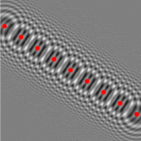
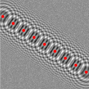
Figure 1: Simulated holograms of spherical particles. On the left-hand side the noiseless signal is displayed. For reconstruction, the noisy signal on the right-hand side is used. The dots correspond to the true location of the particles. The existence of a suitable regularization parameter is guaranteed by condition (26) of proposition 6.1 and hence the $\ell^{1}$-penalized Tikhonov regularization recovered all particles exactly.

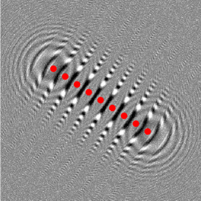
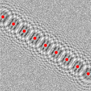
Figure 2: Simulated holograms of spherical particles. In the left column the noiseless signals are displayed. For reconstruction, the noisy signals of the right column are used. The dots correspond to the true location of the particles. The existence of a suitable regularization parameter cannot be shown with condition (26) of proposition 6.1, however, it is possible to find a regularization parameter so that the $\ell^{1}$-penalized Tikhonov regularization recovered all particles exactly. The reason why condition (26) is not fulfilled is that in the image on top the particles have a too small distance to each other, and at the bottom the image was manipulated with unrealistically huge noise.

7 Conclusion

With the papers [16] and [17], the analysis of a priori parameter rules for $\ell^{1}$-penalized Tikhonov functionals seemed completed. On the common parameter rule $\alpha\asymp\varepsilon$, linear, i.e. best possible, convergence is guaranteed. In this paper we have gone beyond this question by presenting a parameter rule which ensures exact recovery of the unknown support of $u^{\scriptscriptstyle\lozenge}\in\ell^{0}$. Moreover, on that condition we achieve a linear convergence rate measured in the $\ell^{1}$ norm, that comes with a-priori checkable error constants which are easier to handle than the ones from [16]. A side product of our analysis is the proof of convergence in $\ell^{0}$ in the topology of sparse convergence.

Section 5 analyzes some implications between different condition for exact recovery. However, in most cases it remains open whether the reverse implications also hold and we postpone this investigation to future work.

Granted, to apply the Neumann $\varepsilon$ERC (20) and the Neumann parameter rule (21) one has to know the support $I$. However, with a certain prior knowledge the correlations

$$\operatorname{COR}_{I}:=\sup\limits_{i\in I}\sum\limits_{\begin{array}[]{c}\scriptstyle j\in I\\ \scriptstyle j\neq i\end{array}}|\langle Ke_{i},Ke_{j}\rangle|\quad\text{and}\quad\operatorname{COR}_{I^{\complement}}:=\sup\limits_{i\in I^{\complement}}\sum\limits_{j\in I}|\langle Ke_{i},Ke_{j}\rangle|,$$

can be estimated from above a priori, especially when the support $I$ is not known exactly. That way it is possible to obtain a priori computable conditions for exact recovery. In section 6 it has be done exemplarily for characteristic functions convolved with a Fresnel function. This shows the practical relevance of the condition.

References

References

- [1] Kristian Bredies and Dirk A. Lorenz. Linear convergence of iterative soft-thresholding. Journal of Fourier Analysis and Applications, 14(5–6):813–837, 2008.
- [2] Emmanuel J. Candés and Justin K. Romberg. Sparsity and incoherence in compressive sampling. Inverse Problems, 23(3):969–985, 2007.
- [3] Emmanuel J. Candés, Justin K. Romberg, and Terence Tao. Stable signal recovery from incomplete and inaccurate measurements. Communications on Pure and Applied Mathematics, 59(8):1207–1223, 2006.
- [4] Emmanuel J. Candés and Terence Tao. Decoding by linear programming. IEEE Transaction on Information Theory, 51(12):4203–4215, 2005.
- [5] Scott Shaobing Chen, David L. Donoho, and Michael A. Saunders. Atomic decomposition by basis pursuit. SIAM Journal on Scientific Computing, 20(1):33–61, 1998.
- [6] Stephan Dahlke, Massimo Fornasier, and Thorsten Raasch. Multilevel preconditioning for adaptive sparse optimization. Preprint 25, DFG SPP 1324, 2009.
- [7] Ingrid Daubechies, Michel Defrise, and Christine De Mol. An iterative thresholding algorithm for linear inverse problems with a sparsity constraint. Communications in Pure and Applied Mathematics, 57(11):1413–1457, 2004.
- [8] Loïc Denis, Dirk A. Lorenz, Eric Thiébaut, Corinne Fournier, and Dennis Trede. Inline hologram reconstruction with sparsity constraints. Optics Letters, 34(22):3475–3477, 2009.
- [9] Loïc Denis, Dirk A. Lorenz, and Dennis Trede. Greedy solution of ill-posed problems: Error bounds and exact inversion. Inverse Problems, 25(11):115017 (24pp), 2009.
- [10] Jean Dieudonné and Laurent Schwartz. La dualité dans les espaces et . Annales de l’Institute Fourier Grenoble, 1:61–101 (1950), 1949.
- [11] David L. Donoho and Michael Elad. Optimally-sparse representation in general (non-orthogonal) dictionaries via minimization. Proceedings of the National Academy of Sciences, 100:2197–2202, 2003.
- [12] Charles Dossal and Stéphane Mallat. Sparse spike deconvolution with minimum scale. In Proceedings of the First Workshop “Signal Processing with Adaptive Sparse Structured Representations”, 2005.
- [13] Heinz W. Engl, Martin Hanke, and Andreas Neubauer. Regularization of Inverse Problems, volume 375 of Mathematics and its Applications. Kluwer Academic Publishers Group, Dordrecht, 2000.
- [14] Jean-Jacques Fuchs. On sparse representations in arbitrary redundant bases. IEEE Transactions on Information Theory, 50(6):1341–1344, 2004.
- [15] Jean-Jacques Fuchs. Recovery of exact sparse representations in the presence of bounded noise. IEEE Transactions on Information Theory, 51(10):3601–3608, 2005.
- [16] Markus Grasmair, Markus Haltmeier, and Otmar Scherzer. Sparse regularization with penalty term. Inverse Problems, 24(5):055020 (13pp), 2008.
- [17] Markus Grasmair, Markus Haltmeier, and Otmar Scherzer. Necessary and sufficient conditions for linear convergence of -regularization. Report 18, FSP S105, 2009.
- [18] Rémi Gribonval and Morten Nielsen. Highly sparse representations from dictionaries are unique and independent of the sparseness measure. Applied and Computational Harmonic Analysis, 22(3):335–355, 2007.
- [19] Rémi Gribonval and Morten Nielsen. Beyond sparsity: Recovering structured representations by minimization and greedy algorithms. Advances in Computational Mathematics, 28(1):23–41, 2008.
- [20] Roland Griesse and Dirk A. Lorenz. A semismooth Newton method for Tikhonov functionals with sparsity constraints. Inverse Problems, 24(3):035007 (19pp), 2008.
- [21] Bangti Jin, Dirk A. Lorenz, and Stefan Schiffler. Elastic-net regularization: Error estimates and active set methods. Inverse Problems, 25(11):115022 (26pp), 2009.
- [22] Dirk A. Lorenz. Convergence rates and source conditions for Tikhonov regularization with sparsity constraints. Journal of Inverse and Ill-Posed Problems, 16(5):463–478, 2008.
- [23] Lawrence Narici and Edward Beckenstein. Topological vector spaces. Marcel Dekker Inc., New York, 1985.
- [24] Ronny Ramlau and Clemens A Zarzer. On the minimization of a tikhonov functional with a non-convex sparsity constraint. Technical report, Johann Radon Institute for Computational and Applied Mathematics.
- [25] Ferréol Soulez, Loïc Denis, Corinne Fournier, Éric Thiébaut, and Charles Goepfert. Inverse problem approach for particle digital holography: accurate location based on local optimisation. Journal of the Optical Society of America A, 24(4):1164–1171, 2007.
- [26] Ferréol Soulez, Loïc Denis, Éric. Thiébaut, Corinne Fournier, and Charles Goepfert. Inverse problem approach in particle digital holography: out-of-field particle detection made possible. Journal of the Optical Society of America A, 24(12):3708–3716, 2007.
- [27] Dennis Trede. Inverse Problems with Sparsity Constraints: Convergence Rates and Exact Recovery. PhD thesis, Univerität Bremen, 2010.
- [28] Joel A. Tropp. Just relax: Convex programming methods for identifying sparse signals in noise. IEEE Transactions on Information Theory, 52(3):1030–1051, 2006.