Abstract

We outline a general strategy to deal with perturbations in brane world models. We illustrate the method by studying simple 6D brane world compactifications. We introduce the background geometries induced by the branes, and summarize the main physical features observed in the fluctuation spectra. We compare these results with 5D brane world models and the traditional Kaluza-Klein picture.

1 Introduction

Extra dimensions, supersymmetry and branes have become a canonical ingredient in physics beyond the standard model and cosmology. In large part, this is due to their motivation from fundamental theories of high energy physics, in particular string theory. Indeed, if string theory is to describe Nature, we must explain why only four of the ten or eleven spacetime dimensions have been observed.

In the traditional Kaluza-Klein picture, a four dimensional effective field theory is obtained from a higher dimensional one by compactifying the extra dimensions to a very small size, say, the string scale. Then, the higher dimensional fields can be represented by an infinite tower of 4D Kaluza-Klein modes, which are essentially harmonics in the internal manifold. Massless modes, such as the 4D graviton, are separated from the massive modes by a finite mass gap. This renders almost all the modes – and thus the extra dimensions – inaccessible to experiments performed at low energies.

The advent of branes widened our possibilities for hiding the extra dimensions. Some fields (the standard model) may be confined to a brane in large extra dimensions, in which case we say their wave functions are localized on the brane. Gravity, describing the dynamics of spacetime itself, must of course propagate everywhere. However, an effective four dimensional gravitational theory can be obtained if the massless mode of the higher dimensional graviton is exponentially enhanced at our brane, whereas the massive modes are exponentially suppressed. This was shown to happen in the 5D brane world model of Randall-Sundrum [1].

5D brane world models have been extremely well studied. They are quite special, since the branes represent boundaries in the spacetime. Much of the interesting dynamics is due to the warp factor, which appears when solving the gravitational backreaction of the brane. It is exponential in the proper distance from the brane. This gives rise to qualitatively different physics from the traditional Kaluza-Klein picture, such as the possibility of infinitely large extra dimensions. The Randall-Sundrum toy models have by now been realized in more stringy scenarios, and are playing a role in such issues as the moduli stabilization problem, inflation and AdS/CFT.

Indeed, extra dimensions are not only obstacles in our quest to connect string theory to Nature. Together with branes and supersymmetry, they also provide new avenues in which to approach some of the long-standing problems of the standard model of particle physics and cosmology. For instance, the exponential warping induced by codimension one branes, was proposed as a solution to the electroweak hierarchy problem [1]. Two submillimeter sized extra dimensions were also proposed early on as a way to relate the Planck and electroweak scales [2], and together with supersymmetry, may even provide a link between that hierarchy and the cosmological constant problem [3].

In the following, we review some of our recent work exploring 6D brane models [4, 5, 6]. As for 5D, and unlike higher codimensions, the gravitational backreaction of codimension two branes can be solved. In the 5D case, the branes induce step-like singularities in the geometry, whereas in 6D the singularities are conical. The warping, rather than the exponential behaviour in 5D, is only power law. We present various background solutions induced by codimension two branes, and study the spectra of small fluctuations near the backgrounds. This analysis is necessary to establish the stability of the configurations, and also allows one to infer properties of the low energy effective 4D theory, and when and how extra-dimensional physics comes into play.

In the next section, we describe the gravitational backreaction of codimension two branes, and present the configurations to be studied. In Section 3 we outline the strategy for analysing the perturbations, which can actually be applied to more general dimensions and codimensions, and in Section 4 we summarize the main physical results for 6D. Finally, we conclude, by comparing and contrasting 6D brane models with their 5D cousins and the traditional Kaluza-Klein models.

We end this introductory section with a few historical remarks. The idea of a brane world and matter localization on them is rather old and has been discussed in different contexts and with different motivations for more than two decades. In [7] the localization of fermion zero modes on a U(1) vortex was discussed and similar ideas were applied to the discussion of superconducting cosmic strings in [8]. The localization of massless gauge fields on a Euclidean 4-brane have even be applied to construct models of chiral fermions on the lattice [9], and has been extended to include gravitational fields [10]. The application to particle physics and cosmology starts with the papers in [11].

2 Codimension Two Brane Models

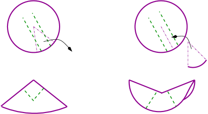
Figure 1: Construction of a cone and saddle-cone by splicing out and in, respectively, a wedge starting from the flat disk. Reproduced from [5]. For the cone, lines that were parallel on the disk remain parallel until they pass on either side of the apex, when they begin to converge. For the saddle-cone they diverge once passing the apex. Notice that although the saddle-cone appears to break the axial-symmetry, this is only an effect of the embedding into 3D. A 2D being would indeed observe the axial symmetry.

A brane in higher dimensional space-time can be introduced with a function $Y^{M}(x)$, which represents the position of the brane [12]. With this function and the bulk metric, $G_{MN}$, we build the induced metric on the brane, $g_{\alpha\beta}=G_{MN}(Y(x))\partial_{\alpha}Y^{M}\partial_{\beta}Y^{N}$, and we can then write an effective brane action of the form:

$$S_{brane}=\int d^{4}x\sqrt{-g}(-T+...),$$ (2.1)

where $T$ is a constant parameter (the tension of the brane) and the dots represent a series of higher derivative terms involving the brane metric and any extra brane localized fields. The total action is then

$$S_{bulk}+S_{brane}.$$ (2.2)

A famous example of this type is the Randall-Sundrum model [1] in which $S_{bulk}$ is the 5D Einstein-Hilbert action with cosmological constant, and one or two branes are included.

Let us discuss in some more detail the 6D case. Henceforth, we assume that any brane localized matter is integrated out, leaving pure tension branes. The simplest choice for the bulk action is the 6D Einstein-Hilbert term

$$S_{EH}=\frac{1}{\kappa^{2}}\int d^{6}X\sqrt{-G}R,$$ (2.3)

where $G$ is the determinant of the higher dimensional metric, and $\kappa$ the 6D Planck scale. For $S_{bulk}=S_{EH}$, a solution of (2.2) with 4D Poincaré invariance is given by the product of the 4D Minkowski space-time and a cone

$$ds^{2}=\eta_{\mu\nu}dx^{\mu}dx^{\nu}+dr^{2}+\left(1-\frac{\delta}{2\pi}\right)^{2}r^{2}d\varphi^{2}.$$ (2.4)

The cone, whose metric is given above in polar coordinates, can be constructed by splicing out a wedge starting from a flat space (see the example on the left in Figure 1). The size of the deficit angle, $\delta$, is related to the brane physics through

$$\delta=\frac{\kappa^{2}T}{2}.$$ (2.5)

The space remains flat apart from at the apex, where the Ricci scalar acquires a delta-function behaviour. Since the deficit angle is bounded from above by $2\pi$, we have an upper bound on the brane tensions that can be described with these mild conical singularities. At the same time, the solution in (2.4) is valid also when $\delta<0$. Negative deficit angles are perfectly well defined, and can even be made at home with a piece of paper and a pair of scissors. A cone with negative deficit angle, which we call saddle-cone, is obtained by splicing a wedge into a flat space (see the example on the right in Figure 1). It is clear that the deficit angle can even take arbitrarily large negative values. Meanwhile, the instabilities generically associated with negative tension branes may be avoided by placing them on orbifold fixed points, which projects out the unstable “branon” modes.

A simple generalization of the bulk action (2.3) is obtained by adding a 6D cosmological constant $\Lambda$ and Yang-Mills gauge fields $\mathcal{A}$, with field strength $F$:

$$S_{bulk}=\int d^{6}X\sqrt{-G}\left(\frac{1}{\kappa^{2}}R-\Lambda-\frac{1}{4}F^{2}\right).$$ (2.6)

This allows for the simplest models of flux compactifications (relevant in moduli stabilization), an example of which is given by the following “rugby-ball” solution, in spherical-polar coordinates [13]:

$$ds^{2}=\eta_{\mu\nu}dx^{\mu}dx^{\nu}+\mathcal{R}^{2}\left(d\theta^{2}+\alpha^{2}\sin^{2}\theta d\varphi^{2}\right),\quad\mathcal{A}=\frac{cQ}{2}(\cos\theta\pm 1)d\varphi\equiv A_{\pm}.$$ (2.7)

Here, $Q$ is a generator of an Abelian subgroup of a simple factor of the gauge group.

In order for (2.7) to be a solution to the equations of motion the constants $\mathcal{R}$, $\alpha$ and $c$ have to fulfil $c=2\sqrt{2}\mathcal{R}\alpha/\kappa$, $\mathcal{R}^{2}=1/(\kappa^{2}\Lambda)$. Thus we see that the size of the extra dimensions is fixed. The metric has two conical singularities at $\theta=0$ and $\theta=\pi$, with deficit angles $\delta=2\pi\left(1-|\alpha|\right)$, which are sourced by two branes of equal tension as in Eq. (2.5).

Figure 2: The rugby-ball. Two patches are needed to describe this geometry. The representations of the gauge field in the two patches, $A_{+}$ and $A_{-}$, have to be related by a single valued gauge transformation, which leads to the Dirac quantization condition.

Finally, topological arguments, which are explained in Figure 2 and its caption, lead to the so called Dirac quantization condition, which for a field interacting with $\mathcal{A}$ through a charge $e$ gives

$$\overline{g}ec\equiv N=\mbox{integer},$$ (2.8)

where $\overline{g}$ is the gauge coupling constant of the subgroup generated by $Q$. The limit $\alpha\rightarrow 1$ (which is equivalent to the limit of zero deficit angle or zero tension) corresponds to a smooth flux compactification on a sphere with radius $\mathcal{R}$ [14].

As motived in the introduction, it is also interesting to consider more sophisticated models, with local supersymmetry in the bulk. 6D chiral gauged supergravity [15], with its positive definite scalar potential, provides a supersymmetric version of the Einstein-Yang-Mills systems discussed above. The bosonic sector includes, additionally, a dilaton $\phi$ and a 2-form field $B_{MN}$, which emerge from the graviton multiplet and an antisymmetric tensor multiplet [15]. Besides the fermionic fields needed to supersymmetrize this bosonic field content, one can also add a number of hypermultiplets ($\Phi$, $\Psi$) - with hyperscalars and hyperinos respectively. The bulk action (for vanishing hyperscalars) is then

$$S_{bulk}= \int d^{6}X\sqrt{-G}\left\{\frac{1}{\kappa^{2}}\left[R-\frac{1}{4}\left(\partial\phi\right)^{2}\right]-\frac{1}{4}e^{\phi/2}F^{2}-\frac{\kappa^{2}}{48}e^{\phi}H_{MNP}H^{MNP}-\frac{8g_{1}^{2}}{\kappa^{4}}e^{-\phi/2}\right\}$$ (2.9)

$$+\rm{fermion\,\,terms},$$

where

$$H_{MNP}=\partial_{M}B_{NP}+F_{MN}{\cal A}_{P}-\frac{g}{3}{\cal A}_{M}\left({\cal A}_{N}\times{\cal A}_{P}\right)+\,\rm{2\,\,cyclic\,\,perms}\,,$$ (2.10)

and $g_{1}$ is the gauge coupling of the $U(1)_{R}$ gauged R-symmetry.

The chiral fermions present in the theory generically lead to gravitational and gauge anomalies, which can sometimes be cancelled by the Green-Schwarz mechanism [16]. This places an attractive restriction on the matter content of the model, and in Table 1 we give some examples of the anomaly free models that have been discovered.

Gauge Group	Hyperino Representation
$E_{7}\times E_{6}\times U(1)_{R}$	$({\bf 912},{\bf 1})_{0}$
$E_{7}\times G_{2}\times U(1)_{R}$	$({\bf 56},{\bf 14})_{0}$
$F_{4}\times Sp(9)\times U(1)_{R}$	$({\bf 52},{\bf 18})_{0}$

Table 1: Some examples of anomaly free models with gauge groups containing $SU(3)\times SU(2)\times U(1)$ [16, 17, 18]. There are also many other models [19].

String theory derivations of 6D chiral supergravity have been provided [20] and its vacuum structure has been investigated in great detail. Gibbons, Güven and Pope (GGP) proved [21] that the only smooth solution of the minimal (anomalous) model, with maximal symmetry in 4D, is the unwarped 4D Minkowski spacetime, with an internal spherical geometry supported by a non vanishing gauge flux [22]. As soon as 3-branes are introduced, conical singularities are generated and the most general solution with 4D maximal symmetry, axial symmetry in the internal space and only those mild conical singularities, has been derived [21, 23]. We consider this class of solutions here and refer to it as the GGP solution. It has the form (notice the flat 4D slices; for an explicit expression see e.g. [6]).

$$ds^{2} = e^{A(\theta)}\left(\eta_{\mu\nu}dx^{\mu}dx^{\nu}+\mathcal{R}^{2}d\theta^{2}\right)+C(\theta)d\varphi^{2}$$

$$\mathcal{A} = \mathcal{A}_{\varphi}(\theta)d\varphi,\quad\phi=\phi(\theta),\quad H=0,$$

Without warping ($A=0$) the internal space is a rugby ball. The warping deforms this solution, and allows brane sources of different tensions. However, the topology of the internal space is still that of the sphere and so we have a Dirac quantization condition, which relates the brane tensions via a topological relation. Almost all the solutions spontaneously break the bulk supersymmetry. The supersymmetric configurations are unwarped, with the monopole flux embedded in the $U(1)_{R}$ gauged R-symmetry, monopole number $N=1$, and brane tensions such that $\delta=0,-2\pi,-4\pi,\dots$.

3 General Perturbations

We now examine the small perturbations about the brane world solutions. For simplicity, in this review we focus on the non-susy 6D model (2.6) and its rugby ball solution, but the scheme presented can be applied to other situations, such as the supersymmetric models described above [4, 5, 6] (see also [24, 25, 26, 27]), the 5D Randall-Sundrum models or indeed smooth Kaluza-Klein compactifications.

Perturbing the solution

$$G_{MN}\rightarrow G_{MN}+h_{MN},\,\,\mathcal{A}_{M}\rightarrow\mathcal{A}_{M}+V_{M},\,\,\mbox{and}\,\,Y^{M}\rightarrow Y^{M}+\xi^{M}$$

one obtains a bilinear action for the perturbations $h_{MN},V_{M}$ and $\xi^{M}$, which has local symmetries descending from the 6D general covariance, the 6D gauge symmetry and the brane general covariance. We fix the first two symmetries by imposing the light cone gauge condition

$$h_{-M}=0,\,\,V_{-}=0.$$ (3.11)

We fix instead the latter symmetry by requiring the static gauge (that is $\xi^{\mu}=0$). In these gauges, perturbations with different helicity decouple [28], and one can examine separately massless and massive gravitons [6], vectors and gauge invariance [4, 6], scalars [5, 6] and fermions [4].

The graviton sector is particularly simple as the corresponding bilinear action is proportional to

$$\int d^{6}X\sqrt{-G}\,\partial_{M}h\partial^{M}h,$$ (3.12)

where we have understood the Lorentz indices on the perturbations. The corresponding equations of motion are

$$\partial_{M}\left(\sqrt{-G}\,\partial^{M}h\right)=0.$$ (3.13)

In deriving this equation we have demanded that a boundary term vanishes; this leads to boundary conditions [29, 30]. The system can then be translated into an equivalent Schroedinger problem, which can be solved explicitly despite the presence of conical singularities. The boundary conditions, together with the requirement of finite kinetic energy for the fluctuations, lead to a discrete mass spectrum:

$$M^{2}=\frac{1}{\mathcal{R}^{2}}({\bf n}+|{\bf m}|\omega)({\bf n}+|{\bf m}|\omega+1),$$

where $\omega\equiv 1/\alpha$, and ${\bf n}=0,1,2,...$ and ${\bf m}=0,\pm 1,\pm 2$ are the Kaluza-Klein wave-numbers. The wave functions can be expressed in terms of the hypergeometric functions (see [4, 6] for details). These results can be used to compute the interactions mediated by massive gravitons on the brane [27].

A similar technique can be applied to analyze the fields with different spin. In the supersymmetric models, we encounter apparently formidable systems of coupled 2nd order differential systems. The smaller systems can be solved in the full generality of the warped models, and even the large ones can be tackled in the unwarped case, with the development of so-called ”rugby ball harmonics”.

4 Results

We now present the main features of 6D brane worlds revealed by our analysis of their perturbations. It is interesting to compare and contrast their behaviour with standard Kaluza-Klein compactifications and 5D brane worlds.

Zero modes

The standard lore of Kaluza-Klein theory (with or without branes) is that any zero modes in the bosonic perturbation spectrum can be identified due to the symmetries of the theory and background solution. This is indeed the case in 6D models with positive tension branes or with a smooth internal space (see e.g. [31]). General coordinate invariance in 4D gives rise to a zero mode for the metric, the axial isometry in 2D gives rise to a massless gauge field, and the classical scaling symmetry, $G_{MN}\rightarrow\lambda\,G_{MN}$ and $e^{\phi}\rightarrow\lambda\,e^{\phi}$, and two-form gauge symmetry, $B\rightarrow B+d\Omega$, each give rise to a massless scalar.

In contrast, in particular models with negative tension branes, extra massless vector fields appear in the spectrum, due to the presence of infinitesimal isometries in the internal space. The massless vector fields are gauge fields in the low energy 4D effective theory obtained by truncating the massive modes. However, the massive modes do not fall into well-defined representations of the corresponding gauge group, so it is not a genuine Kaluza-Klein gauge symmetry group. This can be understood as not all the infinitesimal isometries can be integrated to genuine isometries. Therefore, we expect the extra massless vector fields to remain massless only at the classical level.

Meanwhile, for the fermionic zero modes, it is well known that massless chiral fermions do not generically arise in smooth Kaluza-Klein compactifications. One way to obtain them is by turning on a non-trivial topological configuration for a gauge field background, such as a monopole flux [14]. Negative decifit angles in 6D brane models provide another mechanism for making massless fermions [32]. At the same time, the orbifold projections that feature in the 5D Randall-Sundrum models and models with negative tension branes also lead to chirality.

Mass gap

The compactness of the internal spaces studied ensure that any zero modes are separated from the rest of the spectrum by a mass gap. In standard Kaluza-Klein theory (and 5D brane worlds) as the volume of the extra dimensions is taken to infinity, and mass gap goes to zero. Again, this is also what is observed in 6D models with positive tension branes.

The presence of negative tensions allows for another possibility. If the volume is made large by taking large negative deficit angles, the mass gap can remain large too! In principle, this allows for the possibility of even the Standard Model fields to propagate in large extra dimensions.

Wave function localization

In 5D brane worlds, it is possible that the heavy Kaluza-Klein modes are hidden due to their wave function being suppressed at the position of the brane, where zero modes are instead exponentially enhanced. In 6D, there is a universal asymptotic behaviour for all modes in a given tower. This can be inferred from the potential in the effective Schroedinger problem, in which all dependence on the Kaluza-Klein wave number is dominated at the boundaries by divergences due to the conical defects.

Stability

For the brane configurations discussed to be of interest, they should be stable to small perturbations. Indeed, most of the sectors are free of tachyonic or ghost instabilities. The only sector in which instabilities may lurk are the scalar fluctuations, $V_{m}$, descending from the 6D gauge fields and charged under the background monopole.

	Zero Modes	Mass Gap	Wave Function
Kaluza-Klein	due to symmetries	goes to zero with	massless and massive
		infinite volume	modes have
			same behaviour
5D Brane Worlds	due to symmetries	goes to zero with	massless modes may
		infinite volume	be localized on
			different brane
			to massive modes
6D Brane Worlds	due to symmetries	goes to zero with	massless and massive
($T>0$)		infinite volume	modes have
			same behaviour
6D Brane Worlds	massless modes may	can remain finite	massless and massive
($T<0$)	also arise due to	with infinite volume	modes have
	infinitesimal isometries		same behaviour

Table 2: Comparison of traditional Kaluza-Klein models, 5D Randall-Sundrum like models, and 6D models with positive tension branes only and with negative tension branes. In 5D Randall-Sundrum models, an effective 4D theory may be obtained even with infinitely large extra dimensions, due to the wave function localization properties of the graviton spectrum. In contrast, with negative tension branes, all the Kaluza-Klein massive modes can be hidden in 6D models, due to the mass gap.

The source of the instability is the monopole flux in a non-Abelian gauge sector, and it is to be found also in smooth sphere compactifications [33]. It turns out that models that are stable for the sphere, are also stable in the presence of positive tension branes. This includes all models in which the monopole is embedded in an Abelian gauge group, even if they are non-supersymmetric. Curiously, the introduction of negative tensions can render an unstable monopole flux stable.

Possible endpoints of these instabilities have been studied in [34].

5 Conclusions

We have reviewed the physics of 6D brane worlds, focusing on the background geometries that they induce and the behaviour of their perturbations. In the series of papers [4, 5, 6] we developed a fairly comprehensive analysis of the perturbations in (warped) brane world compactifications of 6D chiral supergravity. The techniques developed could also applied to other scenarios, with different dimensions and codimensions.

Our results show that the behaviour of bulk fluctuations in 6D brane worlds, with positive tensions, is much the same as in traditional Kaluza-Klein compactifications. Moreover, the power law warping that appears in 6D changes the physics little with respect to unwarped models. Instead, models with negative tension branes can lead to new physics. In Table 2 we provide a summary, which compares and contrasts the behaviour amongst Kaluza-Klein models, 5D Randall-Sundrum like models and the 6D models discussed here.

For details, we encourage the reader to refer to [6].

Acknowledgments. The work of A. S. has been supported by CICYT-FEDER-FPA2008-01430. S. L. P. is supported by the Göran Gustafsson Foundation.

References

- [1] L. Randall and R. Sundrum, Phys. Rev. Lett. 83 (1999) 3370 [arXiv:hep-ph/9905221]. L. Randall and R. Sundrum, Phys. Rev. Lett. 83 (1999) 4690 [arXiv:hep-th/9906064].
- [2] N. Arkani-Hamed, S. Dimopoulos and G. R. Dvali, Phys. Lett. B 429 (1998) 263 [arXiv:hep-ph/9803315]. I. Antoniadis, N. Arkani-Hamed, S. Dimopoulos and G. R. Dvali, Phys. Lett. B 436 (1998) 257 [arXiv:hep-ph/9804398].
- [3] Y. Aghababaie, C. P. Burgess, S. L. Parameswaran and F. Quevedo, Nucl. Phys. B 680 (2004) 389 [arXiv:hep-th/0304256]. C. P. Burgess, AIP Conf. Proc. 743 (2005) 417 [arXiv:hep-th/0411140].
- [4] S. L. Parameswaran, S. Randjbar-Daemi and A. Salvio, Nucl. Phys. B 767, 54 (2007) [arXiv:hep-th/0608074].
- [5] S. L. Parameswaran, S. Randjbar-Daemi and A. Salvio, JHEP 0801 (2008) 051 [arXiv:0706.1893 [hep-th]].
- [6] S. L. Parameswaran, S. Randjbar-Daemi and A. Salvio, JHEP 0903 (2009) 136 [arXiv:0902.0375 [hep-th]].
- [7] R. Jackiw and P. Rossi, Nucl. Phys. B 190 (1981) 681.
- [8] E. Witten, Nucl. Phys. B 249 (1985) 557.
- [9] R. Narayanan and H. Neuberger, Nucl. Phys. B 443 (1995) 305 [arXiv:hep-th/9411108]. S. Randjbar-Daemi and J. A. Strathdee, Nucl. Phys. B 443 (1995) 386 [arXiv:hep-lat/9501027].
- [10] S. Randjbar-Daemi and J. A. Strathdee, Phys. Rev. D 51 (1995) 6617 [arXiv:hep-th/9501012].
- [11] V. A. Rubakov and M. E. Shaposhnikov, Phys. Lett. B 125 (1983) 136. V. A. Rubakov and M. E. Shaposhnikov, Phys. Lett. B 125 (1983) 139.
- [12] R. Sundrum, Phys. Rev. D 59 (1999) 085009 [arXiv:hep-ph/9805471].
- [13] S. M. Carroll and M. M. Guica, arXiv:hep-th/0302067. I. Navarro, JCAP 0309, 004 (2003) [arXiv:hep-th/0302129].
- [14] S. Randjbar-Daemi, A. Salam and J. A. Strathdee, Nucl. Phys. B 214 (1983) 491.
- [15] H. Nishino and E. Sezgin, Phys. Lett. B 144 (1984) 187.
- [16] S. Randjbar-Daemi, A. Salam, E. Sezgin and J. A. Strathdee, Phys. Lett. B 151 (1985) 351. S. Randjbar-Daemi and E. Sezgin, Nucl. Phys. B 692 (2004) 346 [arXiv:hep-th/0402217].
- [17] S. D. Avramis, A. Kehagias and S. Randjbar-Daemi, JHEP 0505 (2005) 057 [arXiv:hep-th/0504033].
- [18] S. D. Avramis and A. Kehagias, JHEP 0510 (2005) 052 [arXiv:hep-th/0508172].
- [19] R. Suzuki and Y. Tachikawa, J. Math. Phys. 47, 062302 (2006) [arXiv:hep-th/0512019].
- [20] M. Cvetic, G. W. Gibbons and C. N. Pope, Nucl. Phys. B 677 (2004) 164 [arXiv:hep-th/0308026].
- [21] G. W. Gibbons, R. Guven and C. N. Pope, Phys. Lett. B 595 (2004) 498 [arXiv:hep-th/0307238].
- [22] A. Salam and E. Sezgin, Phys. Lett. B 147 (1984) 47.
- [23] Y. Aghababaie et al., JHEP 0309 (2003) 037 [arXiv:hep-th/0308064].
- [24] C. P. Burgess, C. de Rham, D. Hoover, D. Mason and A. J. Tolley, JCAP 0702 (2007) 009 [arXiv:hep-th/0610078].
- [25] A. Salvio, arXiv:hep-th/0701020.
- [26] H. M. Lee and A. Papazoglou, Nucl. Phys. B 792 (2008) 166 [arXiv:0705.1157 [hep-th]].
- [27] A. Salvio, Phys. Lett. B 681 (2009) 166 [arXiv:0909.0023 [hep-th]].
- [28] S. Randjbar-Daemi and M. Shaposhnikov, Nucl. Phys. B 645 (2002) 188 [arXiv:hep-th/0206016].
- [29] H. Nicolai and C. Wetterich, Phys. Lett. B 150 (1985) 347.
- [30] G. W. Gibbons and D. L. Wiltshire, Nucl. Phys. B 287, 717 (1987) [arXiv:hep-th/0109093].
- [31] S. Randjbar-Daemi, A. Salvio and M. Shaposhnikov, Nucl. Phys. B 741 (2006) 236 [arXiv:hep-th/0601066]. A. Salvio, AIP Conf. Proc. 881 (2007) 58 [arXiv:hep-th/0609050].
- [32] J. M. Schwindt and C. Wetterich, Phys. Lett. B 578 (2004) 409 [arXiv:hep-th/0309065].
- [33] S. Randjbar-Daemi, A. Salam and J. A. Strathdee, Phys. Lett. B 124 (1983) 345 [Erratum-ibid. B 144 (1984) 455]. G. R. Dvali, S. Randjbar-Daemi and R. Tabbash, Phys. Rev. D 65 (2002) 064021 [arXiv:hep-ph/0102307].
- [34] C. P. Burgess, S. L. Parameswaran and I. Zavala, arXiv:0812.3902 [hep-th].