Abstract

An improved method is presented for the numerical evaluation of multi-loop integrals in dimensional regularization. The technique is based on Mellin-Barnes representations, which have been used earlier to develop algorithms for the extraction of ultraviolet and infrared divergencies. The coefficients of these singularities and the non-singular part can be integrated numerically. However, the numerical integration often does not converge for diagrams with massive propagators and physical branch cuts. In this work, several steps are proposed which substantially improve the behavior of the numerical integrals. The efficacy of the method is demonstrated by calculating several two-loop examples, some of which have not been known before.

1 Introduction

Perturbation theory is one of the most important tools for the calculation of particle physics observables. In many cases, radiative corrections are important to match the experimental precision. General and efficient techniques for the computation of one-loop corrections have been developed over many years, resulting in automated frameworks for the calculation of processes with up to six external legs [1]. Most methods for one-loop corrections reduce the loop integrals to a well-defined set of master integrals by Passarino-Veltman and Melrose reduction [2], integration-by-parts and Lorentz-invariance relations [3], or on-shell cut techniques [4]. See Ref. [5] and references therein for a more detailed overview.

In some cases, however, one-loop corrections are not sufficient and two- or even three-loop corrections becomes relevant. Typical examples are electroweak precision observables [6, 7] and production of gauge bosons [8], top quarks [9, 10] or Higgs bosons [11] at the Large Hadron Collider (LHC). Many highly complex calculations have been performed for this purpose by several authors (see references in previous sentence), involving specialized techniques tailored to each particular process. For two-loop amplitudes with a small number of different mass and momentum scales one can follow the traditional approach of reduction to a small number of master integrals, which are then calculated analytically. However, this strategy does not work for applications with a large number of different scales, due to the complexity of the expressions and the fact that in general the master integrals cannot be determined analytically beyond the one-loop level.

Fully numerical techniques for the evaluation of two- and higher-loop integrals face two main challenges: extraction of ultraviolet (UV) and infrared and collinear (IR) singularities, as well as stability and efficiency of the numerical integrations. Methods based on dispersion relations [12, 7] and integrations over Feynman parameters [13] result in low-dimensional numerical integrals with good convergence properties, but they do not offer a general algorithm for the isolation of divergencies. Two powerful approaches for a straightforward extraction of $1/(4-D)$ poles in dimensional regularization are sector decomposition [14] and Mellin-Barnes representations [16, 17, 15]. However, these methods lead to complicated multi-dimensional numerical integrals, which have convergence problems for diagrams with physical branch cuts. For sector decomposition, the instability related to physical branch cuts can be circumvented by the integration contour deformation proposed in Ref. [18].

This article instead focuses on the numerical integration of Mellin-Barnes (MB) representations. Compared to sector decomposition, MB representations of Feynman integrals have the advantage that they typically lead to substantially shorter expressions in the integrand. However, MB representation will only become a viable general tool for numerical two-loop integrations if the behavior of the numerical integrals can be substantially improved. In this paper, several techniques for this purpose are presented, which can also be used in combination to optimize the convergence properties of the integrals. In particular, complex variable transformations and relations that reduce the number of integration dimensions prove to be very useful.

Section 2 starts out by reviewing the employment of MB representations for loop integrals and explaining the origin of the numerical instabilities in the MB integrals. In section 3 the new methods to deal with these instabilities are described in detail. Numerical results for several examples of two-loop integrals are presented in section 4. Where applicable, they are compared to existing results in the literature, which have been obtained by other methods. In addition, results are shown for some integrals appearing in the calculation of two-loop QCD corrections to $gg\to t\bar{t}$ which have not been calculated before. Finally, the main findings are summarized in section 5.

2 Mellin-Barnes representations

The following discussion of the construction of MB representations and the isolation of UV and IR singularities is largely based on Ref. [16]. Let us start with a one-loop $n$-point integral

$$I_{1}=\int\frac{d^{D}q}{i\pi^{D/2}}\,\Bigl{[}[q^{2}-m_{0}^{2}]^{\mu_{0}}[(q+p_{1})^{2}-m_{1}^{2}]^{\mu_{1}}\cdots[(q+p_{1}+p_{2}+\ldots+p_{n})^{2}-m_{n}^{2}]^{\mu_{n}}\Bigr{]}^{-1}$$ (1)

and its Feynman parametrization

$$I_{1}=(-1)^{M} \frac{\Gamma(M-D/2)}{\Gamma(\nu_{0})\cdots\Gamma(\nu_{n})}\int_{0}^{1}dx_{0}\cdots dx_{n}\;\delta(1-x_{0}-\ldots-x_{n})$$ (2)

$$\times\frac{x_{0}^{\mu_{0}-1}\cdots x_{n}^{\mu_{n}-1}}{\left[-\sum_{i,j=1}^{n}(p_{i}-p_{j})^{2}x_{i}x_{j}-\sum_{i=1}^{n}(p_{i}^{2}x_{i}^{2}-m_{i}x_{i})+m_{0}x_{0}-i\epsilon\right]^{M-D/2}},$$

where $M=\mu_{0}+\dots+\mu_{n}$. The integrand denominator can be transformed into a MB representation by

$$\frac{1}{(A_{0}+\ldots+A_{m})^{Z}}=\frac{1}{(2\pi i)^{m}}\int_{{\cal C}_{1}}dz_{1}\cdots \int_{{\cal C}_{m}}dz_{m}\;A_{1}^{z_{1}}\cdots A_{m}^{z_{m}}A_{0}^{-Z-z_{1}-\ldots-z_{m}}$$ (3)

$$\times\frac{\Gamma(-z_{1})\cdots\Gamma(-z_{m})\Gamma(Z+z_{1}+\ldots+z_{m})}{\Gamma(Z)}$$

where the following two conditions must be met:

1. The integration contours ${\cal C}_{i}$ for $z_{i}$ are straight lines parallel to the imaginary axis chosen such that all arguments of the gamma functions have positive real parts.

2. The $A_{i}$ are complex numbers with $|\arg(A_{i})-\arg(A_{j})|<\pi$ for any pair $i,j$.

Satisfying the second condition potentially requires some adjustments of the Feynman parametrization. For example, the scalar diagram in Fig. 1 is represented by the Feynman integral

$$I_{1}^{\rm fig\ref{fig:top1}}=\Gamma(4-\tfrac{D}{2})\int_{0}^{1}dx_{0}dx_{1}dx_{2}dx_{3}\,\frac{\delta(1-x_{0}-x_{1}-x_{2}-x_{3})}{\left[-sx_{1}x_{3}-tx_{0}x_{2}+m^{2}x_{2}-m^{2}x_{1}x_{2}-m^{2}x_{2}x_{3}-i\epsilon\right]^{4-\frac{D}{2}}},$$ (4)

where the terms with $m^{2}$ violate condition 2 above. More generally, problems with the application of the MB representation arise if one mass or momentum parameter appears both with positive and negative signs in the denominator of the Feynman integral. This complication can be avoided by using the relation $\sum_{i}x_{i}=1$. In the case of eq. (4), this relation allows to rewrite it as

$$I_{1}^{\rm fig\ref{fig:top1}}=\Gamma(4-\tfrac{D}{2})\int_{0}^{1}dx_{0}dx_{1}dx_{2}dx_{3}\,\frac{\delta(1-x_{0}-x_{1}-x_{2}-x_{3})}{\left[-sx_{1}x_{3}-tx_{0}x_{2}+m^{2}x_{0}x_{2}+m^{2}x_{2}^{2}-i\epsilon\right]^{4-\frac{D}{2}}},$$ (5)

so that all terms with $m^{2}$ now have positive signs. The term $-sx_{1}x_{3}$ does not lead to any difficulties since one can imagine to temporarily shift $s$ slightly off the real axis into the complex plane so that $|arg(-sx_{1}x_{3})|<\pi$ is satisfied. Thus the Mellin-Barnes formula can be safely applied to eq. (5).

Figure 1: Scalar box diagram corresponding to eq. (4). Thick lines indicate propagators with mass $m$, while thin lines are massless, and external legs are constrained to be on-shell.

After the introduction of the MB representation, the integration over the Feynman parameters can be carried out straightforwardly, using

$$\int_{0}^{1}dx_{0}\cdots dx_{n}\;\delta(1-x_{0}-\ldots-x_{n})\,x_{0}^{\alpha_{0}-1}\cdots x_{n}^{\alpha_{n}-1}=\frac{\Gamma(\alpha_{0})\cdots\Gamma(\alpha_{n})}{\Gamma(\alpha_{0}+\ldots+\alpha_{n})},$$ (6)

assuming that the exponents satisfy

$${\rm Re}(\alpha_{i})>0.$$ (7)

A MB representation for a two-loop integral can be obtained by first deriving a MB representation for one sub-loop, as described above, and inserting the result into the second loop, which then can be transformed into a MB representation with the same procedure. In general, the MB representation for the first sub-loop will contain invariants depending on the second loop momentum, which can be interpreted as new propagators for the second integration.

Figure 2: “Sunset” two-loop diagram. As before, all propagators are assumed to be scalars.

As an example, consider the “sunset” diagram in Fig. 2. The MB representation for the upper sub-loop is given by

$$I_{1}^{\rm fig\ref{fig:sunset},sub}=\frac{1}{(2\pi i)^{2}}\int dz_{1}dz_{2}\, (m_{1}^{2})^{-\varepsilon-z_{1}-z_{2}}(m_{2}^{2})^{z_{2}}(-q_{2}^{2})^{z_{1}}\;\Gamma(-z_{1})\Gamma(-z_{2})\Gamma(1+z_{1}+z_{2})$$

$$\times\frac{\Gamma(1-\varepsilon-z_{2})\Gamma(\varepsilon+z_{1}+z_{2})}{\Gamma(2-\varepsilon+z_{1})},$$ (8)

where $\varepsilon=(4-D)/2$ and $q_{2}$ is the internal momentum of the second (lower) loop. For the second integration one then obtains

$$I_{2}^{\rm fig\ref{fig:sunset}} =\frac{1}{(2\pi i)^{2}}\int dz_{1}dz_{2}\,\int\frac{d^{D}q_{2}}{i\pi^{D/2}}\,\Bigl{[}[q^{2}]^{-z_{1}}[(q_{2}+p)^{2}-m_{3}^{2}]\Bigr{]}^{-1}$$

$$\times(- 1)^{z_{1}}(m_{1}^{2})^{-\varepsilon-z_{1}-z_{2}}(m_{2}^{2})^{z_{2}}\;\Gamma(-z_{1})\Gamma(-z_{2})\Gamma(1+z_{1}+z_{2})\frac{\Gamma(1-\varepsilon-z_{2})\Gamma(\varepsilon+z_{1}+z_{2})}{\Gamma(2-\varepsilon+z_{1})},$$ (9)

so that the $(q_{2}^{2})^{z_{1}}$ gives rise to a new propagator. After constructing the MB representation for the second loop, the final result is

$$I_{2}^{\rm fig\ref{fig:sunset}}= \;\frac{-1}{(2\pi i)^{3}}\int dz_{1}dz_{2}dz_{3}\,(m_{1}^{2})^{-\varepsilon-z_{1}-z_{2}}(m_{2}^{2})^{z_{2}}(m_{3}^{2})^{1-\varepsilon+z_{1}-z_{3}}(-p^{2})^{z_{3}}\;\Gamma(-z_{2})\Gamma(-z_{3})$$

$$\;\times\Gamma(1+z_{1}+z_{2})\Gamma(z_{3}-z_{1})\frac{\Gamma(1-\varepsilon-z_{2})\Gamma(\varepsilon+z_{1}+z_{2})\Gamma(\varepsilon-1-z_{1}+z_{3})}{\Gamma(2-\varepsilon+z_{3})}.$$ (10)

The MB integral can then be be performed numerically.

As mentioned above, the Mellin-Barnes formula and the Feynman parameter integration require the arguments of all gamma functions to have a positive real part. In general, this requires $\varepsilon$ to differ from zero by a finite amount. When taking the limit $\varepsilon\to 0$, the poles of some gamma functions can cross some of the integration contours, so that one needs to correct for this by picking up the residue of the integrand for crossed each pole. As a result, for $\varepsilon\to 0$ one ends up with the original integral plus a sum of terms with lower integration dimension stemming from these residues. An algorithm for this procedure is described in Refs. [16, 17].

Since for appropriate choices of the contours each integral in this sum is regular, the $1/\varepsilon$ singularities must be contained in the coefficients of these integrals. Therefore this method allows to extract all UV and IR divergencies in a systematic way.

3 Improving numerical convergence

The contour integrations in the MB representation can be parametrized as

$$\int_{{\cal C}_{i}}dz_{i}\,f(z_{i})=i\int_{-\infty}^{\infty}dy_{i}\,f(c_{i}+iy_{i}),$$ (11)

where the $c_{i}$ are real constants. The integrand contains powers of the kinematic and mass invariants as well as gamma functions.

Let us return to the example of the sunset diagram, eq. (10). For Euclidean momentum, $p^{2}<0$, the dependence of the invariants on the integration variables $y_{i}$ is given by simple oscillating exponentials, $e.\,g.$ $(m^{2}_{2})^{iy_{2}}$, while the gamma functions rapidly tend to zero when their arguments take values away from the real axis. Therefore, in this case, the integrals are well behaved for numerical integration, and a moderate finite integration interval $y_{i}\in[-10,10]$ is sufficient to reach a high precision for the result.

However, for physical momentum, $p^{2}>0$, an exponentially growing term appears in the integrand:

$$(-p^{2})^{z_{3}}=(p^{2})^{c_{3}+iy_{3}}(-1-i\epsilon)^{c_{3}+iy_{3}}=(p^{2})^{c_{3}+iy_{3}}e^{-i\pi c_{3}}e^{\pi y_{3}}.$$ (12)

Thus the integrand is an oscillating function with slowly decreasing amplitude for $y_{3}\to\infty$. While the integral is formally convergent, numerical integration routines have difficulties dealing with this situation, since one needs to integrate to very large values of $y_{3}$, $i.\,e.$ over many oscillation periods, to reach acceptable precision. See Fig. 3 for illustration.

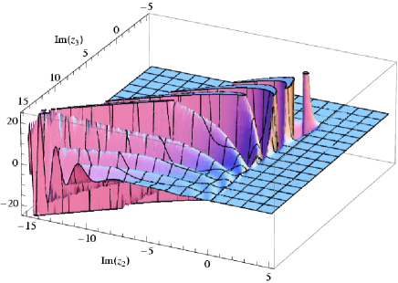
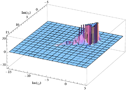
Figure 3: The real part of the integrand for the “sunset” diagram in eq. (10), for $p^{2}=\,$1, $m_{1}^{2}=\,$1, $m_{2}^{2}=\,$4, $m_{3}^{2}=\,$5. For the left panel, the integration contours have been chosen as straight lines parallel to the imaginary axis, and the $z_{1}$ integration has already been carried out. For the right panel, the contours have been deformed by a rotation in the complex plane, corresponding to $\theta=0.4$ in eq. (14).

The problem of slowly converging oscillating tails of the integrand is generic for any MB representation of a loop integral with physical (Minkowski) momenta. Special techniques for numerical integration of oscillating integrands like Filon’s method [19] fail since the oscillation period varies substantially within the integration range. Instead, as shown in the following, suitable variable transformations can substantially improve the convergence properties.

Next, one can exploit the freedom to deform the integration contours in the complex plane, as long as no contour crosses a pole of the integrand. The latter condition is rather restrictive, but if all contours are rotated in the complex plane by the same angle it is guaranteed that no pole crossing occurs:

$$c_{i}+iy_{i}\to c_{i}+(\theta+i)y_{i}.$$ (13)

In eq. (12) this leads to

$$(-p^{2})^{z_{3}}=(p^{2})^{c_{3}+iy_{3}}e^{-i\pi(c_{3}+\theta y_{i})}e^{(\pi+\theta\log p^{2})y_{3}}.$$ (14)

so that the problematic exponential $\exp(\pi y_{3})$ can, in principle, be compensated by the a suitable choice of $\theta$. For the example shown in Fig. 3 (right), it is evident that with this contour deformation the integrand drops off very fast away from the origin, and thus is much better suited for numerical integration.

For a multi-dimensional MB integral, the choice of $\theta$ is more delicate since this one parameter affects all integration variables. It helps to replace the variables $y_{1,\dots,n}$ by hyper-spherical coordinates, $i.\,e.$ $n-1$ angles and one radial coordinate:

$$y_{1} =r\cos\phi_{1},$$ (15)

$$y_{2} =r\sin\phi_{1}\cos\phi_{2},$$

$$\vdots \qquad\qquad\vdots$$

$$y_{n-1} =r\sin\phi_{1}\cdots\sin\phi_{n-2}\cos\phi_{n-1},$$

$$y_{n} =r\sin\phi_{1}\cdots\sin\phi_{n-2}\sin\phi_{n-1}.$$

In this representation, only $r$ is affected by the modification (13) of the integration contours, so that one can in principle choose $\theta$ such that all problematic exponentials of the form (12) are cancelled, as a function of the $\phi_{i}$.

After applying the variable transformations, the multi-dimensional MB integral is sufficiently well-behaved that it can be evaluated with standard Monte-Carlo integration algorithms like Vegas [20]. In particular, the Monte-Carlo error decreases systematically with the number of integration points, which is an important requirement for the convergence of the numerical integration routine.

However, MB integrals with high dimensionality can still require a large amount of computing time to reach a result with acceptable precision. For two-loop diagrams one can obtain MB integrals with more than 10 dimensions, depending on the topology and the number of independent masses and momenta involved. Fortunately, it turns out that in most cases some of the integrations can be performed analytically. For this purpose, the convolution theorem for Mellin transforms proves to be useful. The Mellin transform of a function $f$ is defined as

$${\cal M}[f(x);z]=\int_{0}^{\infty}dx\,f(x)x^{z-1}.$$ (16)

For the Mellin transform of a product of two functions, the convolution theorem then states

$${\cal M}[f(x)g(x);s]=\frac{1}{2\pi i}\int_{c-i\infty}^{c+i\infty}dz\,{\cal M}[f(x);z]\,{\cal M}[g(x);s-z],$$ (17)

where the integration is parallel to the imaginary axis and the integrand in eq. (17) must be analytic for Re$(z)$ in some region around $c$.

With suitable choices of $f$ and $g$ one can derive formulas for MB integrals of two or four gamma functions:

$$\frac{1}{2\pi i}\int_{c-i\infty}^{c+i\infty}dz\,\Gamma(-z)\Gamma(\beta+z)\,t^{z}=\Gamma(\beta)\,(1+t)^{-\beta} \bigl{[}0>c>1-\text{Re}(\beta)\bigr{]}$$ (18)

$$\frac{1}{2\pi i}\int_{c-i\infty}^{c+i\infty}dz\,\Gamma(z)\Gamma(\alpha-z)\Gamma(\beta-z)\Gamma(1-\gamma+z)$$ (19)

$$\quad=\frac{\Gamma(\alpha)\Gamma(\beta)\Gamma(\alpha-\gamma+1)\Gamma(\beta-\gamma+1)}{\Gamma(\alpha+\beta-\gamma+1)} \bigl{[}\text{Re}(\alpha),\,\text{Re}(\beta)>c>0,\,\text{Re}(\gamma)-1\bigr{]}$$

$$\frac{1}{2\pi i}\int_{c-i\infty}^{c+i\infty}dz\,\Gamma(-z)\Gamma(\alpha+z)\Gamma(\beta+z)\Gamma(\gamma-\alpha-z)\,t^{-\alpha-z}$$ (20)

$$\quad=\frac{\Gamma(\alpha)\Gamma(\beta)\Gamma(\gamma)\Gamma(\beta+\gamma-\alpha)}{\Gamma(\beta+\gamma)}\,{}_{2}F_{1}(\alpha,\gamma,\beta+\gamma,1-t) \;\;\bigl{[}0>c>1-\text{Re}(\beta),\,1-\text{Re}(\gamma)\bigr{]}$$

where in each case the contours are assumed to be straight lines parallel to the imaginary axis satisfying the conditions in square brackets, and ${}_{2}F_{1}$ is the Gauss hypergeometric function. These formulas should be applied before the variable transformations. The maximal reduction of the integration dimension is achieved if the formulas are used both before and after the extraction of the $1/\varepsilon$ poles, since in each case one obtains different combinations of terms that match the left-hand sides of eqs. (18)–(20). The reduction procedure has been implemented in a computer algebra program based on Mathematica, which automatically looks for all possible applications of these equations.

4 Examples

In this section numerical results for some examples of scalar two-loop integrals are presented. The generation of the MB representation, the extraction of the $1/\varepsilon$ poles, and the application of the reduction formulas, as described in the previous section, has been implemented in Mathematica. For the numerical integration a C code has been developed, which uses Gaussian quadrature for low dimensionality and the Vegas Monte-Carlo routine for high dimensionality.

In order to test the method and its computer implementation, results will be shown first for several known two-loop integrals, which have been calculated earlier with other methods. A few examples that cannot be computed with any previously published method will be presented at the end of this section.

It should be stressed that all examples in this section cannot be evaluated numerically with MB representations by using the standard representation eq. (11), as implemented $e.\,g.$ in the mb package of Ref. [17], see also Ref. [16]. The reason is that for physical momenta, $p_{i}>0$, the integrands have long oscillating tails that converge too slowly. Therefore, for all cases shown in the following, the variable transformations and contour deformations introduced in the previous sections have been used.

Self-energy topologies:

The scalar sunset diagram in Fig. 2 leads to a three-dimensional MB integral, as shown in section 2, together with one- and two-dimensional integrals originating from pole crossings when the limit $\varepsilon\to 0$ is taken. Expanding in powers of $\varepsilon$, it turns out that the UV poles are given by terms without integrals:

$$I_{2}^{\rm fig\ref{fig:sunset}}=\frac{m_{1}^{2}+m_{2}^{2}+m_{3}^{2}}{2\varepsilon^{2}}+\frac{1}{\varepsilon}\biggl{[}\sum_{i=1}^{3}m_{i}^{2}(\tfrac{3}{2}-\gamma_{E}-\log m_{i}^{2})-\frac{p^{2}}{4}\biggr{]}+I_{2,\rm fin}^{\rm fig\ref{fig:sunset}}.$$ (21)

Numerical results for the finite part are shown in table 1 for two choices of parameters, comparing with values obtained through the dispersion relation method of Ref. [12].

$(p^{2},m_{1}^{2},m_{2}^{2},m_{3}^{2})$	(1, 1, 4, 5)	(16, 2, 2, 1)
Result from MB repr.	18.19558(2)	$17.5083(1)-0.1075(1)i$
(with integration error)
Result from disp. rel.	$18.19559$	$17.50812\phantom{()}-0.10747i$

Table 1: Numerical results for the finite part of the sunset diagram in Fig. 2, obtained with the MB representation method described in this report (second line) and the dispersion relation method of Ref. [12] (third line). Monte-Carlo integration errors for the last quoted digit are given in parentheses. The scale of dimensional regularization has been chosen $\mu=\,$1.

The scalar five-propagator self-energy in Fig. 4 can be cast into a ten-dimensional MB representation, which can be reduced to integrals with dimension up to six with the help of the reduction formulas presented in the previous section. Note that this integral is UV-finite, so that no terms from pole crossings occur.

Figure 4: Five-propagator two-loop diagram. As before, all propagators are assumed to be scalars.

Owing to the relative large dimensionality of the integration, the numerical integration is much slower than in the previous example. With about one hour evaluation time on a single core of a Pentium IV computer with 2.4 GHz a precision of 0.1% to 1% is obtained, depending on the values of the masses and the momentum, see table 2. They compare well with results based on the dispersion relation method of Ref. [12].

$(p^{2},m_{1}^{2},m_{2}^{2},m_{3}^{2},m_{4}^{2},m_{5}^{2})$	($-1$, 1, 1, 1, 1, 1)	(1, 3.7, 3.7, 1, 3.7, 3.7)	(20, 1, 1, 1, 1, 1)
Result from MB repr.	$-0.6809(4)$	$-0.246(2)$	$0.439(1)+0.259(7)i$
(with integration error)
Result from disp. rel.	$-0.68088$	$-0.25421$	$0.43952+0.25365i$

Table 2: Numerical results for the self-energy diagram in Fig. 4, obtained with the MB representation method described in this report (second line) and the dispersion relation method of Ref. [12] (third line). Monte-Carlo integration errors for the last quoted digit are given in parentheses. The scale of dimensional regularization has been chosen $\mu=\,$1.

Vertex topologies:

Figure 5 shows a few examples for two-loop vertex contributions with three or four different scales. The three scalar diagrams lead to MB integrals with 9, 10, and 11 dimensions, respectively, which can be reduced to five dimensions each using the reduction formulas in eqs. (18) ff. In table 3, numerical results are compared with numbers obtained with the dispersion relation method of Refs. [12, 7].

Figure 5: Planar two-loop vertex diagrams which appear as part of the two-loop corrections to $Z\to b\bar{b}$. As before, all propagators are assumed to be scalars, and external legs are constrained to be on-shell.

Diagram	Fig. 5 (a)	Fig. 5 (b)	Fig. 5 (c)
Result from MB repr.	$(2.24(2)+2.34(2)i)\times 10^{-9}$	$1.04(1)\times 10^{-9}$	$3.78(3)\times 10^{-10}$
(with integration error)
Result from disp. rel.	$(2.241\phantom{()}+2.376i)\times 10^{-9}$	$1.036\times 10^{-9}$	$3.805\times 10^{-10}$

Table 3: Numerical results for the vertex diagrams in Fig. 5, obtained with the MB representation method described in this report (second line) and the dispersion relation method of Ref. [12] (third line). Monte-Carlo integration errors for the last quoted digit are given in parentheses. The following values for the masses and regularization scale have been used: $m_{Z}$=91, $m_{W}$=80, $m_{t}$=175, $m_{H}$=100, $\mu$=1.

Box topologies:

This subsection will discuss some two-loop box integrals corresponding to typical topologies for next-to-next-to-leading order QCD corrections to $pp\to t\bar{t}$, shown in Fig. 6. In the diagrams massless (thin) lines correspond to light quark or gluon propagators, while massive (thick) lines indicate top quark propagators.

Figure 6: Some scalar master integrals relevant for two-loop QCD corrections to $pp\to t\bar{t}$. Thick lines indicate massive top-quark propagators, while thin lines are massless, and external legs are constrained to be on-shell.

The master integrals corresponding to (a) and (b) in the figure lead to MB integrals with dimension up to two and three, respectively, after expansion in $\varepsilon$. Therefore they can be evaluated very efficiently with deterministic integration methods, like Gaussian quadrature. These master integrals were computed previously in Ref. [10] with the method of differential equations. Comparing results between the two methods, agreement to more than nine significant digits has been obtained. This comparison was carried out both for an unphysical parameter point with Euclidean momentum $s<0$, as well as for a physical parameter point with $s>(2m_{t})^{2}$. For these cases, the evaluation of the MB integrals takes only several seconds to minutes on a single-core Pentium IV computer.

To the best of our knowledge, the two-loop integral corresponding to Fig. 6 (c) and (d) have not been computed before. Fig. 6 (c) leads to a MB representation with a 13-dimensional integral, which can be reduced to six dimensions with the help of the reduction formulas. Numerical results for a few parameter points are shown in table 4. Since the structure of the integral is rather complicated, the evaluation is much slower than the previous examples. On a single-core Pentium IV computer with 2.4 GHz, the numerical evaluation of one parameter point takes 4-5 hours to reach the precision reported in the table.

$(s,t,m_{t}^{2})$	Result from MB representation $\times 10^{15}$ (with integration error)
$(-100^{2},\,-100^{2},\,175^{2})$	$-2.95397\varepsilon^{-2}+[50.15(1)+0.00(1)i]\varepsilon^{-1}-[515.1(4)-0.0(4)i]$
$\phantom{-}(400^{2},\,-100^{2},\,175^{2})$	$[17.9514-13.6206i]\varepsilon^{-2}+[4720.1(5)-668.5(4)i]\varepsilon^{-1}$
	$\qquad+[3651(13)-1481(13)i]$

Table 4: Numerical results for the box diagram in Fig. 6 (c), obtained with the MB representation method. Monte-Carlo integration errors are given in parentheses. These numbers are based on $m_{t}=\,$175 for the top mass and $\mu=\,$1 for the regularization scale.

Fig. 6 (d) corresponds to a 9-dimensional MB integral, which decomposes into integrals of dimension up to five after application of the reduction formulas and expansion in $\varepsilon$. Table 5 shows numerical results which have been obtained in about 10 hours evaluation time.

$(s,t,m_{t}^{2})$	Result from MB representation $\times 10^{15}$ (with integration error)
$(-100^{2},\,-100^{2},\,175^{2})$	$75.8804\varepsilon^{-3}-[1141.55(5)+0.00(5)i]\varepsilon^{-2}$
	$\qquad+[13338.5(1.4)-0.5(1.4)i]\varepsilon^{-1}-[81900(530)+40(530)i]$
$\phantom{-}(400^{2},\,-100^{2},\,175^{2})$	$[4.17615+12.4156i]\varepsilon^{-3}-[58.04(3)+272.30(3)i]\varepsilon^{-2}$
	$\qquad+[252.3(9)+2932.3(9)i]\varepsilon^{-1}+[742(44)-20649(44)i]$

Table 5: Numerical results for the box diagram in Fig. 6 (d), for the same conditions as in Tab. 4.

5 Summary

Mellin-Barnes representations are a powerful tool for the calculation of multi-loop integrals. They have been shown to be very useful for systematically extracting poles of the form $1/(4-D)$ in dimensional regularization. The coefficients of these poles and the finite part can then be evaluated as numerical integrals. However, for diagrams with massive propagators and physical branch cuts, the integrands a priori can be highly oscillatory, so that standard numerical integration routines do not yield convergent results.

In this article, it is shown how the numerical convergence behavior can be improved substantially by transforming the integration variables, deforming the integration contours in the complex plane, and using analytical formulas to reduce the dimensionality of the integration. The usefulness of those modifications was demonstrated by calculating several examples of two-loop self-energy, vertex and box topologies, some of which have been computed for the first time.

Several previously known techniques permit much faster evaluation of relatively simple multi-loop integrals with few independent masses and momenta than the method presented here. However, Mellin-Barnes representations can be applied in principle to any loop integral, irrespective of its complexity. With sufficient computing time, arbitrarily precise results can be obtained.

In this work, tensor integrals with external uncontracted Lorentz indices were not discussed separately. In fact, for most applications, it is convenient to decompose the loop amplitudes into standard matrix elements or form factors, the coefficients of which only contain scalar integrals. The integrands of these scalar integrals can contain scalar products in the numerator involving on one or more of the loop momenta. Such integrals can be evaluated straightforwardly with Mellin-Barnes representations by expressing the scalar products as propagators with negative powers.

References

-
[1]
A. Denner, S. Dittmaier, M. Roth and L. H. Wieders,
Phys. Lett. B 612, 223 (2005);
A. Denner, S. Dittmaier, M. Roth and L. H. Wieders, Nucl. Phys. B 724, 247 (2005);
T. Binoth, J. P. Guillet, G. Heinrich, E. Pilon and T. Reiter, Comput. Phys. Commun. 180, 2317 (2009);
R. K. Ellis, W. Giele, Z. Kunszt, K. Melnikov, G. Zanderighi, JHEP 0901, 012 (2009);
R. K. Ellis, K. Melnikov and G. Zanderighi, JHEP 0904, 077 (2009);
C. F. Berger et al., Phys. Rev. Lett. 102, 222001 (2009);
C. F. Berger et al., Phys. Rev. D 80, 074036 (2009). -
[2]
D. B. Melrose,
Nuovo Cim. 40, 181 (1965);
G. Passarino and M. J. G. Veltman, Nucl. Phys. B 160, 151 (1979). -
[3]
F. V. Tkachov,
Phys. Lett. B 100, 65 (1981);
K. G. Chetyrkin and F. V. Tkachov, Nucl. Phys. B 192, 159 (1981);
T. Gehrmann, E. Remiddi, Nucl. Phys. B 580, 485 (2000). -
[4]
Z. Bern, L. J. Dixon, D. C. Dunbar and D. A. Kosower,
Nucl. Phys. B 425, 217 (1994);
Z. Bern, L. J. Dixon, D. C. Dunbar and D. A. Kosower, Nucl. Phys. B 435, 59 (1995);
Z. Bern, L. J. Dixon and D. A. Kosower, Phys. Rev. D 73, 065013 (2006);
G. Ossola, C. G. Papadopoulos and R. Pittau, Nucl. Phys. B 763, 147 (2007);
C. Anastasiou, R. Britto, B. Feng, Z. Kunszt and P. Mastrolia, JHEP 0703, 111 (2007);
R. K. Ellis, W. T. Giele and Z. Kunszt, JHEP 0803, 003 (2008);
D. Forde, Phys. Rev. D 75, 125019 (2007);
W. T. Giele, Z. Kunszt and K. Melnikov, JHEP 0804, 049 (2008);
C. F. Berger et al., Phys. Rev. D 78, 036003 (2008). - [5] Z. Bern et al. [NLO Multileg Working Group], in Proc. of the 5th Les Houches Workshop on Physics at TeV Colliders, Les Houches, France, 11-29 Jun 2007, arXiv:0803.0494 [hep-ph].
-
[6]
M. Awramik, M. Czakon, A. Freitas and G. Weiglein,
Phys. Rev. D 69 (2004) 053006;
M. Awramik, M. Czakon, A. Freitas, G. Weiglein, Phys. Rev. Lett. 93, 201805 (2004);
M. Awramik, M. Czakon and A. Freitas, Phys. Lett. B 642, 563 (2006);
W. Hollik, U. Meier and S. Uccirati, Nucl. Phys. B 731, 213 (2005);
W. Hollik, U. Meier and S. Uccirati, Nucl. Phys. B 765, 154 (2007);
M. Awramik, M. Czakon, A. Freitas and B. A. Kniehl, Nucl. Phys. B 813, 174 (2009). - [7] M. Awramik, M. Czakon and A. Freitas, JHEP 0611, 048 (2006).
-
[8]
R. Hamberg, W. L. van Neerven and T. Matsuura,
Nucl. Phys. B 359, 343 (1991)
[Erratum-ibid. B 644, 403 (2002)];
C. Anastasiou, L. Dixon, K. Melnikov and F. Petriello, Phys. Rev. D 69, 094008 (2004);
K. Melnikov and F. Petriello, Phys. Rev. D 74, 114017 (2006). -
[9]
M. Czakon, A. Mitov and S. Moch,
Phys. Lett. B 651, 147 (2007);
M. Czakon, A. Mitov and S. Moch, Nucl. Phys. B 798, 210 (2008);
M. Czakon, Phys. Lett. B 664, 307 (2008);
R. Bonciani, A. Ferroglia, T. Gehrmann, D. Maître and C. Studerus, JHEP 0807, 129 (2008). - [10] R. Bonciani, A. Ferroglia, T. Gehrmann and C. Studerus, JHEP 0908, 067 (2009).
-
[11]
R. V. Harlander and W. B. Kilgore,
Phys. Rev. Lett. 88, 201801 (2002);
C. Anastasiou and K. Melnikov, Nucl. Phys. B 646, 220 (2002);
C. Anastasiou, K. Melnikov and F. Petriello, Phys. Rev. Lett. 93, 262002 (2004);
G. Davatz et al., JHEP 0607, 037 (2006);
S. Catani and M. Grazzini, Phys. Rev. Lett. 98, 222002 (2007);
S. Actis, G. Passarino, C. Sturm and S. Uccirati, Phys. Lett. B 670, 12 (2008). -
[12]
S. Bauberger, F. A. Berends, M. Böhm and M. Buza,
Nucl. Phys. B 434, 383 (1995);
B. A. Kniehl, Acta Phys. Polon. B 27, 3631 (1996). -
[13]
P. Cvitanovic and T. Kinoshita,
Phys. Rev. D 10, 4007 (1974);
A. Ghinculov and J. J. van der Bij, Nucl. Phys. B 436, 30 (1995);
T. Kinoshita and M. Nio, Phys. Rev. D 70, 113001 (2004). -
[14]
T. Binoth and G. Heinrich,
Nucl. Phys. B 585, 741 (2000);
T. Binoth and G. Heinrich, Nucl. Phys. B 680, 375 (2004). -
[15]
V. A. Smirnov,
Phys. Lett. B 460, 397 (1999);
J. B. Tausk, Phys. Lett. B 469, 225 (1999). - [16] C. Anastasiou and A. Daleo, JHEP 0610, 031 (2006).
- [17] M. Czakon, Comput. Phys. Commun. 175, 559 (2006).
-
[18]
Z. Nagy and D. E. Soper,
Phys. Rev. D 74, 093006 (2006);
C. Anastasiou, S. Beerli and A. Daleo, JHEP 0705, 071 (2007). - [19] L. N. G. Filon, Proc. Roy. Soc. Edin. 49, 38 (1928).
- [20] G. P. Lepage, “Vegas: An Adaptive Multidimensional Integration Program,”, report CLNS-80/447 (1980).