Understanding heavy tails in a bounded world or, is a truncated heavy tail heavy or not?

Abstract.

We address the important question of the extent to which random variables and vectors with truncated power tails retain the characteristic features of random variables and vectors with power tails. We define two truncation regimes, soft truncation regime and hard truncation regime, and show that, in the soft truncation regime, truncated power tails behave, in important respects, as if no truncation took place. On the other hand, in the hard truncation regime much of “heavy tailedness” is lost. We show how to estimate consistently the tail exponent when the tails are truncated, and suggest statistical tests to decide on whether the truncation is soft or hard. Finally, we apply our methods to two recent data sets arising from computer networks.

1. Introduction

Probability laws with power tails are ubiquitous in applications. A good fit between empirical distribution of various quantities of interest and distributions with power tails has been reported in such diverse areas as human travel (Brockmann et al., (2006)), earthquake analysis (Corral, (2006)), animal science (Bartumeus et al., (2005)) and even in language (Serrano et al., (2009)). It is also true that in many situations there is a “physical” limit that prevents a quantity of interest from taking an arbitrarily large value. The File Allocation Table (FAT) used on most computer systems allows the largest file size to be 4GB (minus one byte) (Microsoft Knowledge Base Article 154997, (2007)); the greatest loss an insurance company is exposed to by a single covered event is limited by its reinsurance contract (see e.g. Mikosch, (2009)). Even the number of the atoms in the universe is widely considered to be finite. It is common in practice to combine these two facts together and use a model that features power tails only in a truncated form; such models are often referred to as truncated Lévy flights, see e.g. Scholtz and Contreras, (1998), Maruyama and Murakami, (2003) or Zaninetti and Ferraro, (2008). At the first glance this leads to a situation where the power tails, in a sense, completely disappear. The truncation may change dramatically the behavior of the cumulative sums of observations and it always changes dramatically the behavior of the cumulative maxima of the observations. Yet it is precisely such patterns of behavior for which a model with power tails is chosen in the first place. This leads one to ask the natural question: to what extent, if any, do phenomena well described by models with truncated power tails retain the characteristic features of power tails?

Answering this question is not straightforward. We start by pointing out that the level of truncation is linked to the amount of observations one has at hand. This can be thought of in different ways. First of all, finiteness of the sample is sometimes taken as the source of the truncation, see e.g. Burrooughs and Tebbens, (2001) or Barthelemy et al., (2008). Secondly, both the physical nature of the truncation bound and the available data can be linked to a technological level. This is particularly transparent when one models a phenomenon related to computer or communications systems; see e.g. Jelenković, (1999) or Gomez et al., (2000). We describe this situation as a sequence of models, each one with truncated power tails or, in other words, as a triangular array system, which we now proceed to define formally.

Let $F$ be a probability law on ${\mathbb{R}}^{d}$, $d\geq 1$, with the following property. There exists a sequence $(b_{n})$ with $b_{n}\uparrow\infty$ and a non-null Radon measure $\mu$ on $\overline{{\mathbb{R}}^{d}}\setminus\{0\}$ with $\mu\bigl{\{}\overline{{\mathbb{R}}^{d}}\setminus{\mathbb{R}}^{d}\}=0$, such that

(1.1) $$nF\bigl{(}b_{n}^{-1}\cdot\bigr{)}\stackrel{{\scriptstyle v}}{{\longrightarrow}}\mu(\cdot)$$

vaguely in $\overline{{\mathbb{R}}^{d}}\setminus\{0\}$. Here $\overline{{\mathbb{R}}^{d}}$ is the compactification of ${\mathbb{R}}^{d}$ obtained by adding to the latter a ball of infinite radius centered at the origin. The measure $\mu$ has necessarily a scaling property: there exists $\alpha>0$ such that for any Borel set $B\in{\mathbb{R}}^{d}$ and $c>0$, $\mu(cB)=c^{-\alpha}\mu(B)$. We say that the probability law $F$ has regularly varying tails with the tail exponent $\alpha$ (see Resnick, (1987), Hult et al., (2005)), and we view $F$ as the law with non-truncated power tails. When studying the extent to which the central limit theorem behavior is affected by truncation (which is the main point of interest to us in the present paper) we will assume that $0<\alpha<2$. This restriction on the tail exponent $\alpha$ is precisely the one that guarantees that $F$ is in the domain of attraction of an $\alpha$-stable law; see e.g. Rvačeva, (1962). Such a restriction on the values of the tail exponent will not be necessary in other parts of the paper.

For $n=1,2,\ldots$ (regarded both as the number of observations in the $n$th row of the triangular array and the number of the model) let $M_{n}>0$ denote the truncation level. The $n$th row of the triangular array will consist of observations $X_{nj},\,j=1,\ldots,n$, which we view as generated according to the following mechanism:

(1.2) $$X_{nj}:=H_{j}{\bf 1}\bigl{(}\|H_{j}\|\leq M_{n}\bigr{)}+\frac{H_{j}}{\|H_{j}\|}(M_{n}+R_{j}){\bf 1}\bigl{(}\|H_{j}\|>M_{n}\bigr{)}\,,$$

$j=1,\ldots,n,\,n=1,2,\ldots$. Here $H_{1},H_{2},\ldots$ are i.i.d. random vectors in ${\mathbb{R}}^{d}$ with the common law $F$ that has regularly varying tails with a tail exponent $\alpha\in(0,2)$, and $R_{1},R_{2},\ldots$ are an independent of $H_{1},H_{2},\ldots$ sequence of i.i.d. nonnegative random variables. For each $n=1,2,\ldots$ we view the observations $X_{nj},\,j=1,\ldots,n$ as having power tails that are truncated at level $M_{n}$.

We need to comment, at this point, on the role of the random variables $R_{1},R_{2},\ldots$. One should view them as possessing light tails, even exponentially decaying tails. In many cases taking these random variables to be equal to zero with probability 1 is appropriate; in other applications exponentially fast tapering off of the tails beyond the truncation point has been observed (see e.g. Hong et al., (2008)). The reader will notice that the results of this paper hold whenever the tails of the random variables $R_{1},R_{2},\ldots$ are only light enough, not necessarily exponentially light. We have chosen to formulate our results in this way in order to increase their generality, even though we are thinking of their role in the model (1.2) as representing the exponentially fast decaying tails.

Our approach to addressing the question “to what extent do models with truncated power tails retain the characteristic features of power tails?” lies in studying the effect of the rate of growth of the truncation level $M_{n}$ on the asymptotic properties of the triangular array defined in (1.2). Specifically, we introduce the following definition. We will say that the tails in the model (1.2) are

(1.3) $$\begin{array}[]{ll}\text{truncated softly}&\text{if}\ \lim_{n\to\infty}nP\bigl{(}\|H_{1}\|>M_{n}\bigr{)}=0\,,\\ \text{truncated hard}&\text{if}\ \lim_{n\to\infty}nP\bigl{(}\|H_{1}\|>M_{n}\bigr{)}=\infty\,.\end{array}$$

Clearly, an intermediate regime exists as well. Understanding the various aspects of an intermediately truncated model is an interesting theoretical question, that we largely leave aside in this paper, in order to keep its size manageable (see, however, Remark 1 of Section 2). For practical purposes the soft and hard truncation regimes provide the main dichotomy.

We will use fairly classical techniques in Section 2 below to show that, as far as the behavior of the partial sums of the truncated heavy tailed model (1.2) is concerned, observations with softly truncated tails behave like heavy tailed random variables, while observations with hard truncated tails behave like light tailed random variables. It is, however, clear that, in practice, the truncation level $M_{n}$ is not observed. Therefore, we set before ourselves two tasks in this paper. The first one, is to estimate the tail exponent $\alpha$ based on a sample of observations with truncated power tails without knowing the truncation level or, even, if the truncation is soft or hard. We show how this can be accomplished in Section 3. The second task is to find out whether the tails in the sample are truncated softly or hard. In Section 4, where we suggest statistical procedures for testing the hypothesis of the soft (correspondingly, hard) truncation regime against the appropriate alternative. In Section 5 we apply the statistical techniques of Section 4 to two recent data sets related to TCP connections in a large computer network. The goal for that section is only to illustrate the statistical tests discussed in Section 4.

We finish this section by pointing out that some of the issues related to models with power tails that have been “tampered with”, have been addressed in the literature. The goals, points of view or the ways in which the tails are modified were different from what is done in the present work. The paper Asmussen and Pihlsgard, (2005) discusses an application of distributions with truncated power tails in queuing, and addresses the question whether light tailed approximations or heavy approximations work better in this situation. On the other hand, a maximum likelihood estimation procedure of the tail exponent $\alpha$ in a parametric model of truncated power tails (specifically, the truncated Pareto distribution) is given in Aban et al., (2006). Estimation of the tail exponent in randomly censored power models (where the tails are not so much truncated, as contaminated) is discussed in Beirlant et al., (2007) and Einmahl et al., (2008). Finally, the Hill estimator for censored data is discussed in Beirlant and Guillou, (2001). The techniques for dealing with censored tails are consistent with the earlier work of Csörgo et al., (1986).

2. A Central Limit Theorem for random vectors with truncated power tails

Consider the triangular array defined in (1.2), where, as we recall, the random vectors $H_{1},H_{2},\ldots$ have a distribution with regularly varying tails with a tail exponent $\alpha\in(0,2)$. This means that these random vectors (or their law $F$) are in the domain of attraction of some $\alpha$-stable law $\rho$ on ${\mathbb{R}}^{d}$ (see Rvačeva, (1962)). That is, the partial sums $S_{n}^{(H)}=H_{1}+\ldots+H_{n}$, $n=1,2,\ldots$, converge in law, after appropriate centering and scaling, to $\rho$. Defining the sums of the truncated observations,

$$S_{n}:=\sum_{j=1}^{n}X_{nj},\ n=1,2,\ldots\,,$$

we would like to know whether $\bigl{(}S_{n},\,n=1,2,\ldots\bigr{)}$ still converge in law, after suitable centering and scaling, to $\rho$. If the answer is no, then we would like to know what do these sums of random vectors with truncated power tails converge to. These questions can be handled by the classical probabilistic tools, and the answer turns out to depend exclusively on the truncation regime as defined in (1.3).

2.1. Soft truncation regime: truncated heavy tails are still heavy

We start with the situation where the truncation level $M_{n}$ grows sufficiently fast with the sample size, so that the truncated power tails model (1.2) is in the soft truncation regime. Theorem 2.1 below shows that, in this case, the partial sums of the random vectors with truncated heavy tails converge, when properly centered and scaled, to the same $\alpha$-stable limit as without truncation.

Let $(c_{n})$ and $(b_{n})$ denote, respectively, some centering and scaling sequences for the non-truncated random vectors $(H_{j})$, that is,

(2.1) $$b_{n}^{-1}S_{n}^{(H)}-c_{n}=b_{n}^{-1}\sum_{j=1}^{n}H_{j}-c_{n}\Longrightarrow\rho$$

as $n\to\infty$.

Theorem 2.1.

In the soft truncation regime we have

(2.2) $$b_{n}^{-1}S_{n}-c_{n}\Longrightarrow\rho\,.$$

Proof.

By (2.1) it is enough to show that

$$b_{n}^{-1}\left\|S_{n}-\sum_{j=1}^{n}H_{j}\right\|\stackrel{{\scriptstyle p}}{{\longrightarrow}}0\,.$$

However, for any $\varepsilon>0$,

$$P\left(b_{n}^{-1}\left\|S_{n}-\sum_{j=1}^{n}H_{j}\right\|>\varepsilon\right)\leq P\Bigl{(}\|H_{j}\|>M_{n}\ \ \text{for some $j=1,\ldots,n$}\Bigr{)}$$

$$\leq nP\bigl{(}\|H_{1}\|>M_{n}\bigr{)}\to 0\,,$$

and the claim follows. ∎

2.2. Hard Truncation regime: truncated heavy tails are no longer heavy

Now we consider the situation where the truncation level $M_{n}$ grows relatively slowly with the sample size, and that the truncated power tails model (1.2) is in the hard truncation regime. As we will see, in this case the partial sums of the random vectors with truncated heavy tails are no longer asymptotically $\alpha$-stable but, rather, converge in law, after suitable centering and scaling, to a Gaussian limit. Therefore, at least from the point of view of the behavior of partial sums, a model with power tails that have been truncated hard does not behave anymore as a heavy tailed model.

We start with some preliminaries. Recall that, since the limiting law $\rho$ in (2.1) is $\alpha$-stable, the Lévy-Khinchine formula for its characteristic function has the form

(2.3) $$\hat{\rho}(\theta)=\exp\biggl{[}i\langle\theta,\gamma\rangle$$

$$+\int_{S}\left(\int_{0}^{\infty}\left\{e^{ix\langle\theta,s\rangle}-1-ix\langle\theta,s\rangle{\bf 1}(x\leq 1)\right\}x^{-(1+\alpha)}\,dx\right)\Gamma(ds)\biggr{]}$$

for $\theta\in{\mathbb{R}}^{d}$, where $\gamma\in{\mathbb{R}}^{d}$, and $\Gamma$ is a finite measure on the unit sphere in ${\mathbb{R}}^{d}$, $S:=\{x\in{\mathbb{R}}^{d}:\|x\|=1\}$, see Theorem 6.15 in Araujo and Giné, (1980). The measure $\Gamma$ is often referred to as spectral measure of the law $\rho$; see Theorem 2.3.1 in Samorodnitsky and Taqqu, (1994).

Theorem 2.2.

Assume that $ER_{1}^{2}<\infty$, and let

$$B_{n}:=\bigl{[}nM_{n}^{2}P(\|H_{1}\|>M_{n})\bigr{]}^{1/2},\,n=1,2,\ldots\,.$$

Then in the hard truncation regime we have

(2.4) $$B_{n}^{-1}(S_{n}-ES_{n})\Longrightarrow\eta\,,$$

where $\eta$ is a centered Gaussian law on ${\mathbb{R}}^{d}$ whose covariance matrix has the entries

(2.5) $$\frac{2}{2-\alpha}\int_{S}s_{i}s_{j}\,\tilde{\Gamma}(ds),\,i,j=1,\ldots,d\,,$$

where $\tilde{\Gamma}(\cdot):=\Gamma(\cdot)/\Gamma(S)$ is the normalized spectral measure of $\rho$.

We start with a lemma.

Lemma 2.1.

For every continuous function $f:S\longrightarrow\mathbb{R}$,

$$\lim_{n\rightarrow\infty}nB_{n}^{-2}\int_{S}\int_{0}^{M_{n}}f(s)r^{2}P\left(\|H_{1}\|\in dr,\frac{H_{1}}{\|H_{1}\|}\in ds\right)=\frac{\alpha}{2-\alpha}\int_{S}f(s)\,\tilde{\Gamma}(ds).$$

Proof.

Assumption (2.1) means that

(2.6) $$\frac{P\left(\|H_{1}\|>r,\,\frac{H_{1}}{\|H_{1}\|}\in\cdot\right)}{P\bigl{(}\|H_{1}\|>r\bigr{)}}\Longrightarrow\tilde{\Gamma}(\cdot)$$

weakly on $S$; see e.g. Corollary 6.20 (b) of Araujo and Giné, (1980). Therefore,

$$\int_{S}\int_{0}^{M_{n}}f(s)r^{2}P\left(\|H_{1}\|\in dr,\frac{H_{1}}{\|H_{1}\|}\in ds\right)$$

$$=\int_{0}^{M_{n}}2y\left(\int_{S}f(s)P\left(\|H_{1}\|>y,\,\frac{H_{1}}{\|H_{1}\|}\in ds\right)\right)dy$$

$$-M_{n}^{2}\int_{S}f(s)P\left(\|H_{1}\|>M_{n},\,\frac{H_{1}}{\|H_{1}\|}\in ds\right)$$

$$\sim\int_{S}f(s)\,\tilde{\Gamma}(ds)\left[\int_{0}^{M_{n}}2yP\bigl{(}\|H_{1}\|>y\bigr{)}\,dy-M_{n}^{2}P\bigl{(}\|H_{1}\|>M_{n}\bigr{)}\right]$$

$$\sim\int_{S}f(s)\,\tilde{\Gamma}(ds)\left(\frac{2}{2-\alpha}-1\right)M_{n}^{2}P\bigl{(}\|H_{1}\|>M_{n}\bigr{)}=n^{-1}B_{n}^{2}\int_{S}f(s)\,\tilde{\Gamma}(ds)$$

as $n\to\infty$, where the second asymptotic equivalence follows from the Karamata theorem (see e.g. Resnick, (1987)). ∎

Proof of Theorem 2.2.

By the Cramér-Wold device it suffices to show that for every $\theta$ in ${\mathbb{R}}^{d}$,

$$B_{n}^{-1}\bigl{(}\langle\theta,S_{n}\rangle-E\langle\theta,S_{n}\rangle\bigr{)}\Rightarrow N\left(0,\frac{2}{2-\alpha}\int_{S}\langle\theta,s\rangle^{2}\tilde{\Gamma}(ds)\right)\,.$$

To this end we will use the Central Limit Theorem for triangular arrays under the Lindeberg condition; see e.g. Theorem 2.4, page 345 in Gut, (2005). We need to prove that

(2.7) $$\lim_{n\to\infty}\frac{n}{B_{n}^{2}}{\rm Var}\bigl{(}\langle\theta,X_{n1}\rangle\bigr{)}=\frac{2}{2-\alpha}\int_{S}\langle\theta,s\rangle^{2}\tilde{\Gamma}(ds)$$

and that for every $\varepsilon>0$,

(2.8) $$\frac{n}{B_{n}^{2}}E\biggl{(}\bigl{|}\langle\theta,X_{n1}\rangle-E\bigl{(}\langle\theta,X_{n1}\rangle\bigr{)}\bigr{|}^{2}{\bf 1}\Bigl{(}\bigl{|}\langle\theta,X_{n1}\rangle-E\bigl{(}\langle\theta,X_{n1}\rangle\bigr{)}\bigr{|}>\varepsilon B_{n}\Bigr{)}\biggr{)}\to 0$$

as $n\to\infty$. In order to prove (2.7), we will show that

(2.9) $$\lim_{n\to\infty}\frac{n}{B_{n}^{2}}E\bigl{(}(\langle\theta,X_{n1}\rangle)^{2}\bigr{)}=\frac{2}{2-\alpha}\int_{S}\bigl{(}\langle\theta,s\rangle\bigr{)}^{2}\tilde{\Gamma}(ds)$$

while

(2.10) $$\lim_{n\to\infty}\frac{n^{1/2}}{B_{n}}\bigl{|}E\bigl{(}\langle\theta,X_{n1}\rangle\bigr{)}\bigr{|}=0\,.$$

The former claim follows easily from Lemma 2.1 and the weak convergence (2.6) by writing

$$E\bigl{(}(\langle\theta,X_{n1}\rangle)^{2}\bigr{)}=E\Bigl{(}(\langle\theta,H_{1}\rangle)^{2}{\bf 1}\bigl{(}\|H_{1}\|\leq M_{n}\bigr{)}\Bigr{)}$$

$$+E\left(\frac{\bigl{(}\langle\theta,H_{1}\rangle\bigr{)}^{2}}{\|H_{1}\|^{2}}(M_{n}+R_{1})^{2}{\bf 1}\bigl{(}\|H_{1}\|>M_{n}\bigr{)}\right)$$

$$\sim n^{-1}B_{n}^{2}\frac{\alpha}{2-\alpha}\int_{S}\bigl{(}\langle\theta,s\rangle\bigr{)}^{2}\,\tilde{\Gamma}(ds)+\bigl{(}1+o(1)\bigr{)}M_{n}^{2}E\left(\frac{\bigl{(}\langle\theta,H_{1}\rangle\bigr{)}^{2}}{\|H_{1}\|^{2}}{\bf 1}\bigl{(}\|H_{1}\|>M_{n}\bigr{)}\right)$$

$$\sim n^{-1}B_{n}^{2}\frac{\alpha}{2-\alpha}\int_{S}\bigl{(}\langle\theta,s\rangle\bigr{)}^{2}\,\tilde{\Gamma}(ds)+M_{n}^{2}P\bigl{(}\|H_{1}\|>M_{n}\bigr{)}\int_{S}\bigl{(}\langle\theta,s\rangle\bigr{)}^{2}\,\tilde{\Gamma}(ds)$$

$$=n^{-1}B_{n}^{2}\left(\frac{\alpha}{2-\alpha}+1\right)\int_{S}\bigl{(}\langle\theta,s\rangle\bigr{)}^{2}\,\tilde{\Gamma}(ds)=n^{-1}B_{n}^{\alpha}\frac{\alpha}{2-\alpha}\int_{S}\bigl{(}\langle\theta,s\rangle\bigr{)}^{2}\,\tilde{\Gamma}(ds)\,.$$

For (2.10) we write

$$\bigl{|}E\bigl{(}\langle\theta,X_{n1}\rangle\bigr{)}\bigr{|}\leq\|\theta\|\Bigl{[}E\bigl{(}\|H_{1}\|{\bf 1}(\|H_{1}\|\leq M_{n})\bigr{)}+M_{n}P\bigl{(}\|H_{1}\|>M_{n}\bigr{)}\Bigr{]}\,.$$

Since

$$M_{n}P\bigl{(}\|H_{1}\|>M_{n}\bigr{)}\ll M_{n}\bigl{(}P(\|H_{1}\|>M_{n})\bigr{)}^{1/2}=n^{-1/2}B_{n}\,,$$

the claim (2.10) will follow once we check that

(2.11) $$\lim_{n\rightarrow\infty}n^{1/2}B_{n}^{-1}E\left[\|H_{1}\|{\bf 1}(\|H_{1}\|\leq M_{n})\right]=0\,.$$

We give separate arguments for the cases $\alpha\leq 1$ and $\alpha>1$.
Case 1 ($\alpha\leq 1$): Letting $C$ be a positive constant whose value may change from line to line, by the Karamata theorem,

$$E\left[\|H_{1}\|{\bf 1}(\|H_{1}\|\leq M_{n})\right] \leq \bigl{(}E\left[\|H_{1}\|^{3/2}{\bf 1}(\|H_{1}\|\leq M_{n})\right]\bigr{)}^{2/3}$$

$$\sim CM_{n}\bigl{(}P(\|H_{1}\|>M_{n})\bigr{)}^{2/3}$$

$$= Cn^{-1/2}B_{n}\bigl{(}P(\|H_{1}\|>M_{n})\bigr{)}^{1/6}$$

$$\ll n^{-1/2}B_{n}\,.$$

Case 2 ($1<\alpha<2$): Here (2.11) follows trivially from the fact that $E\left[\|H_{1}\|{\bf 1}(\|H_{1}\|\leq M_{n})\right]$ has a finite limit, while $B_{n}\gg n^{1/2}$ as $\alpha<2$.

We have now proved (2.7). By (2.10), the remaining condition (2.8) will follow once we check that for every $\varepsilon>0$,

$$\frac{n}{B_{n}^{2}}E\Bigl{(}\bigl{|}\langle\theta,X_{n1}\rangle\bigr{|}^{2}{\bf 1}\bigl{(}\bigl{|}\langle\theta,X_{n1}\rangle\bigr{|}>\varepsilon B_{n}\bigr{)}\Bigr{)}\to 0\,.$$

This is, however, an immediate consequence of the fact that the hard truncation implies that $B_{n}\gg M_{n}$ as $n\to\infty$. ∎

Remark 1.

We briefly address the behavior of the partial sums of the random vectors with truncated heavy tails in the intermediate regime

(2.12) $$\lim_{n\rightarrow\infty}nP(\|H\|>M_{n})=\delta\in(0,\infty)\,.$$

It turns out that, in this case, one can use the same centering and scaling sequences $\{c_{n}\}$ and $\{b_{n}\}$ as in the non-truncated case (2.1) (or in the soft truncation regime (2.2)), but the limit will be different. In fact,

(2.13) $$b_{n}^{-1}S_{n}-c_{n}\Longrightarrow\rho_{\delta}\,,$$

where $\rho_{\delta}$ is an infinitely divisible law on ${\mathbb{R}}^{d}$, which is obtained by a certain truncation of the jumps of the $\alpha$-stable law $\rho$ in (2.3). Specifically,

(2.14) $$\hat{\rho}_{\delta}(\theta)=\exp\biggl{[}i\langle\theta,\gamma_{\delta}\rangle$$

$$+\int_{S}\biggl{(}\int_{0}^{\delta^{-1/\alpha}(\alpha^{-1}\Gamma(S))^{1/\alpha}}\left\{e^{ix\langle\theta,s\rangle}-1-ix\langle\theta,s\rangle{\bf 1}(x\leq 1)\right\}x^{-(1+\alpha)}\,dx$$

$$+\delta\Gamma(S)^{-1}\left\{e^{i\delta^{-1/\alpha}(\alpha^{-1}\Gamma(S))^{1/\alpha}\langle\theta,s\rangle}-1\right\}\biggr{)}\Gamma(ds)\biggr{]}$$

for $\theta\in{\mathbb{R}}^{d}$, where

$$\gamma_{\delta}=\gamma-\int_{\delta^{-1/\alpha}(\alpha^{-1}\Gamma(S))^{1/\alpha}}^{\infty}x^{-\alpha}{\bf 1}(x\leq 1)\,dx\int_{S}s\,\Gamma(ds)\,.$$

We sketch the argument. Write

(2.15) $$b_{n}^{-1}S_{n}-c_{n}=\left(b_{n}^{-1}\sum_{j=1}^{n}H_{j}{\bf 1}\bigl{(}\|H_{j}\|\leq M_{n}\bigr{)}-c_{n}\right)$$

$$+b_{n}^{-1}M_{n}\sum_{j=1}^{n}\frac{H_{j}}{\|H_{j}\|}{\bf 1}\bigl{(}\|H_{j}\|>M_{n}\bigr{)}+b_{n}^{-1}\sum_{j=1}^{n}\frac{H_{j}}{\|H_{j}\|}R_{j}{\bf 1}\bigl{(}\|H_{j}\|>M_{n}\bigr{)}\,.$$

It is easy to check that the last term in the right hand side of (2.15) converges to zero in probability. Since (2.12) implies that

(2.16) $$\frac{M_{n}}{b_{n}}\to\delta^{-1/\alpha}(\alpha^{-1}\Gamma(S))^{1/\alpha}$$

as $n\to\infty$, Theorem 5.9, p. 129, of Araujo and Giné, (1980) implies that the first term in the right hand side of (2.15) has a weak limit whose characteristic function is given by

$$\exp\biggl{[}i\langle\theta,\gamma_{\delta}\rangle$$

$$+\int_{S}\biggl{(}\int_{0}^{\delta^{-1/\alpha}(\alpha^{-1}\Gamma(S))^{1/\alpha}}\left\{e^{ix\langle\theta,s\rangle}-1-ix\langle\theta,s\rangle{\bf 1}(x\leq 1)\right\}x^{-(1+\alpha)}\,dx\biggr{)}\Gamma(ds)\biggr{]}\,.$$

Finally, it follows from (2.16) that the second term in the right hand side of (2.15) is asymptotically equivalent to

$$\delta^{-1/\alpha}(\alpha^{-1}\Gamma(S))^{1/\alpha}\sum_{j=1}^{n}\frac{H_{j}}{\|H_{j}\|}{\bf 1}\bigl{(}\|H_{j}\|>M_{n}\bigr{)}\,,$$

and, by (2.6) and (2.12), the sum above converges weakly to the law of the Poisson sum $\sum_{j=1}^{N}Y_{j}$, where $Y_{1},Y_{2},\dots$ are i.i.d. $S$-valued random variables with the common law $\tilde{\Gamma}$, and $N$ is an independent of them Poisson random variable with mean $\delta$. Since the weak limits of the first and the second terms in the right hand side of (2.15) are easily seen to be independent, this shows (2.13).

3. Hill estimator for random variables with truncated power tails

Estimating the tail exponent $\alpha$ is one of the main statistical issues one faces when working with data for which a model with power tails is contemplated. This is a difficult statistical problem because one attempts to estimate a parameter governing the tail behavior in an otherwise nonparametric model. By necessity, any estimator one uses has to be based on a vanishing fraction of the available data. The situation is even trickier when one tries to estimate the tail exponent in a sample of observations with truncated power tails. This is the task we address in this section.

The formal setup in this section is as follows. We are given a sample $X_{1},\ldots,X_{n}$ of one-dimensional nonnegative observations from the model with truncated power tails, i.e. (1.2). We emphasize a slight change in notation from (1.2): whereas the latter used the notation $X_{n1},\ldots,X_{nn}$ to emphasize the triangular array nature of the model, in a statistical procedure, when a single sample (i.e., a particular row of the triangular array) is given, the notation $X_{1},\ldots,X_{n}$ is more natural. The discussion in Section 2 makes it intuitive that estimating the tail exponent $\alpha$ should be easier if the tails are truncated softly, than in the case when the tails are truncated hard. This is, indeed, the case. However, in this section we are interested in finding a procedure that permits consistent estimation of the tail exponent $\alpha$ regardless of the truncation regime; this is especially important because the truncation regime is never known (see, however, Section 4 below). Furthermore, in this section we do not restrict the values of the tails exponent to the interval $(0,2)$. That is, $\alpha$ can take any positive value.

A number of estimators of the tail exponent of distributions with nontruncated power tails have been suggested; a thorough discussion can be found in Chapter 4 of de Haan and Ferreira, (2006). One of the best known and widely used estimators is the Hill estimator introduced by Hill, (1975). Given a sample $X_{1},\ldots,X_{n}$. the Hill statistic is defined by

(3.1) $$h_{n,k}=\frac{1}{k}\sum_{i=1}^{k}\log\frac{X_{(i)}}{X_{(k)}}\,,$$

where $X_{(1)}\geq X_{(2)}\geq\ldots\geq X_{(n)}$ are the order statistics from the sample $X_{1},\ldots,X_{n}$, and $k=1,\ldots,n$ is a user-determined parameter, the number of the upper order statistics to use in the estimator. The consistency result for the Hill estimator says that, if $X_{1},\ldots,X_{n}$ are i.i.d. with regularly varying right tail with exponent $\alpha>0$, and $k=k_{n}\to\infty$, $k_{n}/n\to 0$ as $n\to\infty$, then $h_{n,k_{n}}\to 1/\alpha$ in probability as $n\to\infty$; see e.g. Theorem 3.2.2 in de Haan and Ferreira, (2006).

In spite of the simplicity of the statement of the consistency of the Hill estimator, selecting the number $k$ of the upper order statistics for a given sample with nontruncated power tails remains a daunting problem; see e.g. pp. 192-193 in Embrechts et al., (1997). In the main result of this section, Theorem 3.1 below, we will see that one has to be particularly careful when using the Hill estimator on a sample with truncated power tails. Nonetheless, a consistent estimator can still be obtained.

Notice that the next theorem does not impose any conditions on the random variables $R_{1},R_{2},\ldots$ in the model (1.2).

Theorem 3.1.

Suppose that the number $k_{n}$ of the upper order statistics satisfies

(3.2) $$nP(H_{1}>M_{n})+1\ll k_{n}\ll n\,.$$

Then $h_{n,k_{n}}\to 1/\alpha$ in probability as $n\to\infty$.

Note that Theorem 3.1 says that, in the soft truncation regime, the Hill estimator is consistent under the same assumption, $k_{n}/n\to 0$, as in the nontruncated case.

Proof.

For simplicity, we write $k$ instead of $k_{n}$. An inspection of the proof of consistency of the Hill estimator in the nontruncated case in e.g. Resnick, (2007) shows that the result will follow once we check that, under the conditions of the theorem,

(3.3) $$\frac{n}{k}P\left[\frac{X_{n1}}{b(n/k)}\in\cdot\right]\stackrel{{\scriptstyle v}}{{\longrightarrow}}\mu(\cdot)$$

vaguely in $(0,\infty]$, where $\mu$ is a measure on $(0,\infty]$ defined by

$$\mu((x,\infty])=x^{-\alpha}\mbox{ for all }x>0\,,$$

and

$$b(u)=\inf\bigl{\{}x>0:\,P(H_{1}>x)\leq u^{-1}\bigr{\}},\,u>0\,.$$

Note that $(b(n))$ is no longer necessarily a sequence satisfying (2.1). In fact, we will use this notation several times in the sequel to denote other quantile-type functions associated with the random variable $H_{1}$.

By the hypothesis,

$$\lim_{n\rightarrow\infty}\frac{n}{k}P(H_{1}>M_{n})=0$$

and, hence, $b(n/k)\ll M_{n}$ as $n\to\infty$. Therefore, for any $x>0$, for $n$ large enough,

$$P\left[\frac{X_{n1}}{b(n/k)}>x\right] = P\bigl{(}H_{1}>xb(n/k)\bigr{)}$$

$$\sim \frac{k}{n}x^{-\alpha}$$

where the last line follows from the hypothesis $k\ll n$ and regular variation of the tail of $H_{1}$. This shows (3.3). ∎

Since the truncation level $M_{n}$ is not known, it is desirable to have a sample-based way of deciding on the number of upper order statistics to use in the Hill estimator. A natural (in view of the condition (3.2)) choice is to use a random number of upper order statistics given by

(3.4) $${\hat{k}}_{n}=\left[n\left(\frac{1}{n}\sum_{j=1}^{n}{\bf 1}\bigl{(}X_{j}>\gamma\max_{i=1,\ldots,n}X_{i}\bigr{)}\right)^{\beta}\right]\,,$$

where $\gamma$ and $\beta$ are user-specified parameters taking values in $(0,1)$ and $[\cdot]$ denotes the integer part. The next two theorems show that this choice of the number of upper order statistics leads to a consistent estimator of the reciprocal of the tail exponent. The parameters $\beta$ and $\gamma$ can and should be chosen by the user, and the consistency of the estimator depends neither on their choice nor on, for instance, second order regular variation of $H_{1}$. In practice, one should, probably, use some version of the so-called Hill plot (see e.g. Embrechts et al., (1997)), by calculating the value of the estimator for a range of $\beta$ and $\gamma$. We leave this issue for future work.

We start with proving consistency of the Hill estimator with the random choice of the number of upper order statistics in the hard truncation regime. Here the consistency requires that the tail of the random variable $R_{1}$ is sufficiently light, relatively to the truncation level.

Theorem 3.2.

In the hard truncation regime assume, additionally, that

(3.5) $$P(H_{1}>M_{n})P(R_{1}>\epsilon M_{n})=o(1/n)\ \mbox{ for all }\ \epsilon>0.$$

If $\hat{k}_{n}$ is chosen as in (3.4), then $h_{n,\hat{k}_{n}}\to 1/\alpha$ in probability as $n\to\infty$.

Proof.

We start by showing that, as $n\longrightarrow\infty$,

(3.6) $$\frac{\hat{k}_{n}}{k_{n}}\stackrel{{\scriptstyle P}}{{\longrightarrow}}1\,,$$

where

$$k_{n}:=\left[nP(H_{1}>\gamma M_{n})^{\beta}\right]\,.$$

Clearly, all that needs to be shown is

(3.7) $$\frac{\sum_{j=1}^{n}{\bf 1}(X_{j}>\gamma\hat{M}_{n})}{nP(H_{1}>\gamma M_{n})}\stackrel{{\scriptstyle P}}{{\longrightarrow}}1,$$

where $\hat{M}_{n}:=\max_{1\leq i\leq n}X_{i}$. By (3.5),

(3.8) $$\frac{\hat{M}_{n}}{M_{n}}\stackrel{{\scriptstyle P}}{{\longrightarrow}}1\,.$$

Further, because of the hard truncation,

(3.9) $$\frac{\sum_{j=1}^{n}{\bf 1}\left(j:X_{j}>\theta_{1}M_{n}\right)}{nP(H>\theta_{2}M_{n})}\stackrel{{\scriptstyle P}}{{\longrightarrow}}\left(\frac{\theta_{1}}{\theta_{2}}\right)^{-\alpha}$$

for any $0<\theta_{1}<1$ and $\theta_{2}>0$.

Fix $0<\epsilon<1$. Choose first $0<\eta<1$ be such that $(1-\eta)^{-\alpha}<1+\epsilon$. Writing

$$P\left[\frac{\sum_{j=1}^{n}{\bf 1}\left(X_{j}>\gamma\hat{M}_{n}\right)}{nP(H_{1}>\gamma M_{n})}>1+\epsilon\right]$$

$$\leq P[(1-\eta)M_{n}>\hat{M}_{n}]+P\left[\frac{\sum_{j=1}^{n}{\bf 1}\left(X_{j}>\gamma(1-\eta)M_{n}\right)}{nP(H_{1}>\gamma M_{n})}>1+\epsilon\right]$$

and using (3.8) and (3.9), we see that

$$P\left[\frac{\sum_{j=1}^{n}{\bf 1}\left(X_{j}>\gamma\hat{M}_{n}\right)}{nP(H_{1}>\gamma M_{n})}>1+\epsilon\right]\longrightarrow 0\,.$$

Next we choose $\eta>0$ such that $\gamma(1+\eta)<1$ and $(1+\eta)^{-\alpha}>1-\epsilon$. Writing

$$P\left[\frac{\sum_{j=1}^{n}{\bf 1}\left(X_{j}>\gamma\hat{M}_{n}\right)}{nP(H_{1}>\gamma M_{n})}<1-\epsilon\right]$$

$$\leq P[(1+\eta)M_{n}<\hat{M}_{n}]+P\left[\frac{\sum_{j=1}^{n}{\bf 1}\left(X_{j}>\gamma(1+\eta)M_{n}\right)}{nP(H_{1}>\gamma M_{n})}<1-\epsilon\right]\,,$$

and appealing, once again, to (3.8) and (3.9), we obtain

$$P\left[\frac{\sum_{j=1}^{n}{\bf 1}\left(X_{j}>\gamma\hat{M}_{n}\right)}{nP(H_{1}>\gamma M_{n})}<1-\epsilon\right]\longrightarrow 0\,,$$

which establishes (3.7), and, hence, also (3.6).

In view of (3.6), it suffices to show that

$$\frac{1}{k_{n}}\sum_{i=1}^{\hat{k}_{n}}\log\frac{X_{(i)}}{X_{(\hat{k}_{n})}}\stackrel{{\scriptstyle P}}{{\longrightarrow}}\frac{1}{\alpha}\,.$$

Fix $\epsilon>0$. We choose $0<\eta<1/2$ so that $\alpha^{-1}\log\frac{1+\eta}{1-\eta}<\frac{\epsilon}{3}$, and write

$$P\left[\left|\frac{1}{k_{n}}\sum_{i=1}^{\hat{k}_{n}}\log\frac{X_{(i)}}{X_{(\hat{k}_{n})}}-\frac{1}{\alpha}\right|>\epsilon\right]$$

$$\leq P\left[\left|\frac{1}{k_{n}}\sum_{i=1}^{k_{n}}\log\frac{X_{(i)}}{X_{(k_{n})}}-\frac{1}{\alpha}\right|>\frac{\epsilon}{3}\right]+P\left[-\log\frac{X_{([k_{n}(1+\eta)])}}{X_{([k_{n}(1-\eta)])}}>\frac{\epsilon}{3}\right]$$

$$+P\left[\left|\frac{\hat{k}_{n}}{k_{n}}-1\right|\geq\eta\right]\,.$$

It follows from Theorem 3.1 that

$$P\left[\left|\frac{1}{k_{n}}\sum_{i=1}^{k_{n}}\log\frac{X_{(i)}}{X_{(k_{n}+1)}}-\frac{1}{\alpha}\right|>\frac{\epsilon}{3}\right]\longrightarrow 0\,.$$

Since $k_{n}\gg nP(H_{1}>M_{n})$, we see that

$$\frac{X_{([k_{n}(1+\eta)])}}{X_{([k_{n}(1-\eta)])}}\stackrel{{\scriptstyle P}}{{\longrightarrow}}\left(\frac{1+\eta}{1-\eta}\right)^{-1/\alpha}\,.$$

Therefore, by the choice of $\eta$,

$$P\left[-\log\frac{X_{([k_{n}(1+\eta)])}}{X_{([k_{n}(1-\eta)])}}>\frac{\epsilon}{3}\right]\longrightarrow 0\,.$$

In conjunction with (3.6), this completes the argument. ∎

Next, we show consistency of the Hill estimator using the random number (3.4) of upper order statistics in the soft truncation regime. Note that no assumption on the tail of $R_{1}$ is necessary in this case.

Theorem 3.3.

In the soft truncation regime, if $\hat{k}_{n}$ is chosen as in (3.4), then $h_{n,\hat{k}_{n}}\to 1/\alpha$ in probability as $n\to\infty$.

Proof.

Let $\bigl{(}\tilde{h}(k,n)\bigr{)}$ denote the Hill sequence based on the random variables $H_{1},\ldots,H_{n}$, i.e.

$$\tilde{h}(k,n):=\frac{1}{k}\sum_{i=1}^{k}\log\frac{H_{(i)}}{H_{(k)}}\,,$$

where $1\leq k\leq n$ and $H_{(1)}\geq\ldots\geq H_{(n)}$ are the order statistics of $H_{1},\ldots,H_{n}$. Let $\beta$ be as in (3.4). It is well known that the random step function

$$\left(\tilde{h}([n^{1-\beta}t],n):t\geq 1\right)$$

converges in probability in $D[1,\infty)$, equipped with the topology of uniform convergence on bounded intervals, to the constant deterministic function $c(t)=1/\alpha$ for $t\geq 1$; see Resnick, (2007), page 89. Since

$$P\left(\tilde{h}([n^{1-\beta}t],n)\neq h([n^{1-\beta}t],n)\mbox{ for some }t\geq 1\right)\leq nP(H>M_{n})\longrightarrow 0\,,$$

it follows that

(3.10) $$\left(h([n^{1-\beta}t],n):t\geq 1\right)\stackrel{{\scriptstyle P}}{{\longrightarrow}}\bigl{(}c(t):t\geq 1\bigr{)}$$

in $D[1,\infty)$ as well. By Proposition 3.21 (page 154) in Resnick, (1987) and soft truncation, we known that

$$N_{n}:=\sum_{j=1}^{n}{\bf 1}\bigl{(}X_{j}>\gamma\max_{i=1,\ldots,n}X_{i}\bigr{)}\Longrightarrow N:=\sum_{j=1}^{\infty}{\bf 1}\left(\Gamma_{j}^{-1/\alpha}>\gamma\Gamma_{1}^{-1/\alpha}\right)\,,$$

where $\left(\Gamma_{j}:j\geq 1\right)$ is the sequence of the arrival times of the unit rate Poisson process on $(0,\infty)$. Using (3.10) and Theorem 4.4 (page 27) in Billingsley, (1968) we conclude that

$$\left(h([n^{1-\beta}t],n),\,N_{n}^{\beta}\right)\Longrightarrow\left(\frac{1}{\alpha},\,N^{\beta}\right)$$

in $D[1,\infty)\times{\mathbb{N}}^{\beta}$, where ${\mathbb{N}}^{\beta}:=\{1,2^{\beta},3^{\beta},\ldots\}$. Since the evaluation map from $D[1,\infty)\times{\mathbb{N}}^{\beta}$ to ${\mathbb{R}}$ defined by $(x,a)\mapsto x(a)$ is continuous, an appeal to the continuous mapping theorem finishes the proof. ∎

4. Testing for soft and hard truncation

The first two sections of this paper provide, among other things, evidence that, in certain important respects, random variables with truncated heavy tails retain “most of the tail heaviness” if the truncation is soft, but loose “much of the tail heaviness” if the truncation is hard. Since the truncation level is not observed, how does one decide if the tails of observed data have been truncated softly or hard? In this section we construct statistical tests for testing each of the two hypothesis against the corresponding alternative. As in Section 3 we restrict ourselves to the case of one-dimensional observations and the tail exponent $\alpha$ can take any positive value.

Suppose that we are given a sample $X_{1},\ldots,X_{n}$ of one-dimensional observations from the model (1.2). As in Section 3, we do not use here the triangular array notation. Neither the precise value of the tail exponent nor the exact distribution of the random variables $(R_{n})$ in (1.2) are assumed to be known. However, we will assume that an upper bound on the tail exponent $\alpha$ is known.

This section is split into three subsections, describing, correspondingly, testing the hypothesis of soft truncation, testing the hypothesis of hard truncation, and testing a slightly stronger version of the latter.

4.1. Testing the hypothesis of soft truncation

We consider the following problem of testing a null hypothesis against a simple alternative:

(4.1) $$\left.\begin{array}[]{rcl}H_{0}:&P(|H_{1}|>M)\ll n^{-1}&\mbox{(soft truncation)}\\ H_{\rm alt}:&P(|H_{1}|>M)\gg n^{-1}&\mbox{(hard truncation)}\end{array}\right\}.$$

We assume the tail exponent $\alpha$ satisfies

(4.2) $$\alpha<A<\infty\,,$$

i.e. an upper bound on the tail exponent is available. As a test statistic we will use

(4.3) $$Z_{n}(A):=\frac{\sum_{i=1}^{n}|X_{i}|^{A}}{\max_{1\leq i\leq n}|X_{i}|^{A}}\,.$$

The following proposition describes the asymptotic distribution of $Z_{n}(A)$ under the null hypothesis and under the alternative.

Proposition 4.1.

(i)  Under the hypothesis $H_{0}$ of soft truncation,

(4.4) $$Z_{n}(A)\Rightarrow\Gamma_{1}^{A/\alpha}\sum_{j=1}^{\infty}\Gamma_{j}^{-A/\alpha}\,,$$

where $(\Gamma_{j},\,j\geq 1)$ are the arrival times of a unit rate Poisson process on $(0,\infty)$.

(ii)  Assume that $ER_{1}^{A}<\infty$. Then under the hypothesis $H_{\rm alt}$ of hard truncation, $Z_{n}(A)\stackrel{{\scriptstyle P}}{{\longrightarrow}}\infty$.

Proof.

For part (i), we define

$$b_{n}=\inf\bigl{\{}x>0:\,P(|H_{1}|^{A}>x)\leq n^{-1}\bigr{\}},\,n=1,2,\ldots\,.$$

Note that, for any $x>0$,

$$nP\bigl{(}b_{n}^{-1}|X_{1}|^{A}>x\bigr{)}\sim nP\bigl{(}b_{n}^{-1}|H_{1}|^{A}>x\bigr{)}\to x^{-\alpha}$$

as $n\to\infty$. It follows from Proposition 3.21 (page 154) in Resnick, (1987) that we have the following weak convergence of a sequence of point processes on $(0,\infty]$:

(4.5) $$N_{n}:=\sum_{j=1}^{n}\delta_{b_{n}^{-1}|X_{1}|^{A}}\Rightarrow N:=\sum_{j=1}^{\infty}\delta_{\Gamma_{j}^{-A/\alpha}}$$

as $n\to\infty$. Here $\delta_{a}$ is a point mass at $a$, and the weak convergence takes place in the space of Radon point measures on $(0,\infty]$ endowed with the topology of vague convergence; see Section 3.4 in Resnick, (1987). We would like to use the continuous mapping theorem to deduce (4.4) from (4.5), but a preliminary truncation step is necessary.

For $\varepsilon>0$ we define

$$Z_{n}(A;\varepsilon):=\frac{\sum_{i=1}^{n}|X_{i}|^{A}{\bf 1}\bigl{(}b_{n}^{-1}|X_{i}|^{A}>\varepsilon\bigr{)}}{\max_{1\leq i\leq n}|X_{i}|^{A}}\,.$$

Notice that $Z_{n}(A;\varepsilon)=h(N_{n})$, where for a Radon point measure $\eta=\sum_{j}\delta_{r_{j}}$ on $(0,\infty]$,

$$h(\eta)=\frac{\eta\bigl{(}(\varepsilon,\infty]\bigr{)}}{\max_{j}r_{j}}\,.$$

It is standard (and easy) to check that $h$ is continuous with probability 1 at the Poisson random measure $N$ in (4.5), so by the continuous mapping theorem,

$$Z_{n}(A;\varepsilon)\Rightarrow\Gamma_{1}^{A/\alpha}\sum_{j=1}^{\infty}\Gamma_{j}^{-A/\alpha}{\bf 1}\bigl{(}\Gamma_{j}^{-A/\alpha}>\varepsilon\bigr{)}\,.$$

Therefore, the convergence (4.4) will follow once we check that for every $\delta>0$,

(4.6) $$\lim_{\varepsilon\to 0}\limsup_{n\to\infty}P\bigl{(}Z_{n}(A)-Z_{n}(A;\varepsilon)>\delta\bigr{)}=0\,.$$

To this end, notice that, for any $0<\theta<1$ we can select $\tau>0$ so small that $P\bigl{(}\max_{1\leq i\leq n}|X_{i}|^{A}\leq\tau b_{n}\bigr{)}\leq\theta$ for all $n$ large enough. Then, for all $n$ large enough,

$$P\bigl{(}Z_{n}(A)-Z_{n}(A;\varepsilon)>\delta\bigr{)}\leq\theta+\delta^{-1}E\left(\tau^{-1}b_{n}^{-1}\sum_{i=1}^{n}|X_{i}|^{A}{\bf 1}\bigl{(}b_{n}^{-1}|X_{i}|^{A}\leq\varepsilon\bigr{)}\right)$$

$$=\theta+\delta^{-1}\tau^{-1}nb_{n}^{-1}E\Bigl{(}|X_{1}|^{A}{\bf 1}\bigl{(}b_{n}^{-1}|X_{1}|^{A}\leq\varepsilon\bigr{)}\Bigr{)}$$

$$=\theta+\delta^{-1}\tau^{-1}nb_{n}^{-1}E\Bigl{(}|H_{1}|^{A}{\bf 1}\bigl{(}b_{n}^{-1}|H_{1}|^{A}\leq\varepsilon\bigr{)}\Bigr{)}$$

$$\sim\theta+\delta^{-1}\tau^{-1}nb_{n}^{-1}\Bigl{(}(1-\alpha/A)^{-1}(\varepsilon b_{n})P\bigl{(}|H_{1}|^{A}>\varepsilon b_{n}\bigr{)}$$

$$\sim\theta+\delta^{-1}\tau^{-1}nb_{n}^{-1}(1-\alpha/A)^{-1}(\varepsilon b_{n})\bigl{(}\varepsilon^{-\alpha/A}n^{-1}\bigr{)}$$

$$=\theta+\delta^{-1}\tau^{-1}(1-\alpha/A)^{-1}\varepsilon^{1-\alpha/A}.$$

where the second equality holds because of soft truncation, and the first asymptotic equivalence follows from the Karamata theorem. Since $A>\alpha$, we obtain (4.6) by first letting $\varepsilon\to 0$ and then $\theta\to 0$. This completes the proof of part (i).

For part (ii), we start with observing that

(4.7) $$\frac{\sum_{i=1}^{n}|X_{i}|^{A}}{nM_{n}^{A}P(|H_{1}|>M_{n})}\geq\frac{\sum_{i=1}^{n}|H_{i}|^{A}{\bf 1}\bigl{(}M_{n}/2\leq|H_{i}|\leq M_{n}\bigr{)}}{nM_{n}^{A}P(|H_{1}|>M_{n})}$$

$$\geq(M_{n}/2)^{A}\frac{\sum_{i=1}^{n}{\bf 1}\bigl{(}M_{n}/2\leq|H_{i}|\leq M_{n}\bigr{)}}{nM_{n}^{A}P(|H_{1}|>M_{n})}\sim 2^{-A}(2^{\alpha}-1)$$

in probability. On the other hand, for some constant $c>0$, by the assumption $ER_{1}^{A}<\infty$,

$$\max_{1\leq i\leq n}|X_{i}|^{A}\leq c\bigl{(}M_{n}^{A}+\max_{1\leq j\leq n}R_{j}^{A}\bigr{)}=cM_{n}^{A}+o(1)n$$

a.s. as $n\to\infty$. Since the truncation is hard, and $A>\alpha$, we see that

(4.8) $$\frac{\max_{i=1,\ldots,n}|X_{i}|^{A}}{nM_{n}^{A}P(|H_{1}|>M_{n})}\to 0$$

a.s. as $n\to\infty$ as well. The claim of part (ii) follows from (4.7) and (4.8). ∎

Based on Proposition 4.1, we suggest the following test for the problem (4.1).

(4.9) $$\text{reject $H_{0}$ at significance level $p\in(0,1)$ if}\ \ Z_{n}(A)>c_{p}(\alpha/A)\,,$$

with $c_{p}(\theta)$ such that $P(Z(\theta)>c_{p}(\theta))=p$, where for $0<\theta<1$,

(4.10) $$Z(\theta)=\Gamma_{1}^{1/\theta}\sum_{j=1}^{\infty}\Gamma_{j}^{-1/\theta}\,.$$

The random variable $Z(\theta)$ does not seem to have one of the standard distributions, and we are not aware of any previous studies of the distribution of $Z(\theta)$. The following proposition lists some of the properties of this distribution.

Proposition 4.2.

The random variable $Z(\theta)$ is an infinitely divisible random variable. It has a density with respect to the Lebesgue measure, and the Laplace transform

(4.11) $$Ee^{-\gamma Z(\theta)}=\left(1+\gamma e^{\gamma}\int_{0}^{1}e^{-\gamma x}x^{-\theta}\,dx\right)^{-1}\,,$$

$\gamma>\gamma_{0}$, where $\gamma_{0}<0$ is the number satisfying

$$1+\gamma_{0}e^{\gamma_{0}}\int_{0}^{1}e^{-\gamma_{0}x}x^{-\theta}\,dx=0\,.$$

Proof.

For $\delta>0$ let

$$W_{\delta}=\sum_{j=1}^{\infty}\bigl{(}\delta+\Gamma_{j}\bigr{)}^{-1/\theta}\,.$$

Then $W_{\delta}$ is an infinitely divisible random variable with the Laplace transform

$$Ee^{-\gamma W_{\delta}}=\exp\left\{-\int_{0}^{\delta^{-1/\theta}}\bigl{(}1-e^{-\gamma y}\bigr{)}\theta y^{-(1+\theta)}\,dy\right\}$$

for all $\gamma\in{\mathbb{R}}$ because the Lévy measure of $W_{\delta}$ has a compact support; see Rosiński, (1990) and Sato, (1999). Since

$$Z(\theta)\stackrel{{\scriptstyle d}}{{=}}1+T^{1/\theta}W_{T}$$

where $T$ is a standard exponential random variable independent of $\bigl{(}\Gamma_{j}:j\geq 1\bigr{)}$, it follows that

(4.12) $$Ee^{-\gamma Z(\theta)}=\int_{0}^{\infty}e^{-t}e^{-\gamma}Ee^{-\gamma t^{1/\theta}W_{t}}\,dt$$

$$=e^{-\gamma}\int_{0}^{\infty}e^{-t}\exp\left\{-t\int_{0}^{1}\bigl{(}1-e^{-\gamma x}\bigr{)}\theta x^{-(1+\theta)}\,dx\right\}\,dt$$

$$=e^{-\gamma}\int_{0}^{\infty}\exp\left\{-t\left[e^{-\gamma}+\gamma\int_{0}^{1}e^{-\gamma x}x^{-\theta}\,dx\right]\right\}\,dt$$

via integration by parts. Since the exponent under the integral is positive if and only if $\gamma>\gamma_{0}$, we obtain (4.11). Additionally, it follows from (4.12) that

(4.13) $$Z(\theta)\stackrel{{\scriptstyle d}}{{=}}1+Y(T)\,,$$

where $\bigl{(}Y(t),\,t\geq 0\bigr{)}$ is a subordinator satisfying

(4.14) $$Ee^{-\gamma Y(t)}=\exp\left\{-t\int_{0}^{1}\bigl{(}1-e^{-\gamma x}\bigr{)}\theta x^{-(1+\theta)}\,dx\right\},\ \ t\geq 0\,,$$

independent of $T$. Since a Lévy process stopped at an independent infinitely divisible random time is, obviously, infinitely divisible, so is $Z(\theta)$. Furthermore, the characteristic function of $Y(t)$ is integrable of the real line for every $t>0$, so each $Y(t)$ has a density, and then the same is true for any mixture of $(Y(t))$. Therefore, $Z(\theta)$ has a density. ∎

Even though we know, by Proposition 4.2, that the random variable $Z(\theta)$ has a density, at present we do not know ways to compute this density. One possibility to estimate the critical values $c_{p}(\alpha/A)$ to perform the test (4.9), is as follows. For values of $\alpha$ not too close to the upper bound $A$ (or, equivalently, for the values of $\theta$ not too close to $1$), it is possible to estimate the critical values by the Monte-Carlo method, by truncating the infinite series at a sufficiently large finite number of terms. Using $N=10^{5}$ number of terms in the series and generating the (truncated) random variable $10^{5}$ times, we have estimated the following quantiles, for a range of values $\theta$.

	$0.5$	$0.6$	$0.7$
$.05$	$4.3$	$5.8$	$8.2$
$.025$	$5.1$	$6.9$	$9.8$
$.01$	$6.2$	$8.4$	$12.1$

For $\theta$ closer to $1$, the rate of convergence of the truncated sum $\sum_{j=1}^{N}\Gamma_{j}^{-1/\theta}$ as $N\to\infty$ is very slow, and in order to obtain upper bounds on the quantiles of the random variable $Z(\theta)$ we used Proposition 4.2 as described below. Such upper bounds lead to conservative versions of the test (4.9). We use the exponential Markov inequality: for $0<r<-\gamma_{0}$,

$$P(Z(\theta)\geq z)\leq e^{-rz}Ee^{rZ}=e^{-rz}\left(1-re^{-r}\int_{0}^{1}e^{rx}x^{-\theta}\,dx\right)^{-1}\,,$$

and estimate the integral from above by

$$\int_{0}^{1}e^{rx}x^{-\theta}dx\leq e^{r/k}\frac{k^{\theta-1}}{1-\theta}+\frac{1}{k}\sum_{j=2}^{k}e^{rj/k}\left(\frac{j-1}{k}\right)^{-\theta}\,,$$

$k>1$. Using $r=.05$ and $k=10^{7}$ we computed numbers $\tilde{c}_{p}(\theta)$ satisfying

$$P\bigl{(}Z(\theta)\geq\tilde{c}_{p}(\theta)\bigr{)}\leq p\,.$$

These numbers $\tilde{c}_{p}(\theta)$ are reported in the following table.

	$0.8$	$0.9$	$0.95$
$.05$	$65.43$	$73.12$	$127.37$
$.025$	$79.29$	$86.98$	$141.23$
$.01$	$97.62$	$105.31$	$159.56$

Since we are only assuming that the tail exponent $\alpha$ has a known upper bound as in (4.2), but the exact value of $\alpha$ may be unknown, a possible way to obtain a conservative estimate of the critical value $c_{p}(\alpha/A)$ in (4.10) is to choose a number $A_{1}>A$ and use the statistic $Z_{n}(A_{1})$ instead of $Z_{n}(A)$ in (4.3). By Proposition 4.1, under the null hypothesis, the test statistic converges weakly to $Z(\alpha/A_{1})$, which is stochastically smaller than $Z(A/A_{1})$, and we obtain a conservative test by modifying (4.9) as follows:

(4.15) $$\text{reject $H_{0}$ at significance level $p\in(0,1)$ if}\ \ Z_{n}(A_{1})>c_{p}(A/A_{1})\,.$$

4.2. Testing the hypothesis of hard truncation

In this subsection we consider the following problem of testing a null hypothesis against a simple alternative:

(4.16) $$\left.\begin{array}[]{rcl}H_{0}:&P(|H_{1}|>M)\gg n^{-1}&\mbox{(hard truncation)}\\ H_{\rm alt}:&P(|H_{1}|>M)\ll n^{-1}&\mbox{(soft truncation)}\end{array}\right\}.$$

We still assume that an upper bound (4.2) on the tail exponent is known. For a test statistic in this case we choose a number $\gamma\in(0,1)$ and define

(4.17) $$Z_{n}(A;\gamma)=\frac{\left(\sum_{j=1}^{[\gamma n]}(-1)^{j}X_{j}^{\langle A/2\rangle}\right)^{2}}{\sum_{j=[\gamma n]+1}^{n}|X_{j}|^{A}}.$$

Here $a^{\langle b\rangle}=|a|^{b}{\rm sign}(a)$ for real $a,b$ is the signed power. The asymptotic distribution of $Z_{n}(A;\gamma)$ under the null hypothesis and under the alternative in (4.16) is described in Proposition 4.3 below. Recall the standard notation of $S_{\alpha}(\sigma,\beta,\mu)$ for (the distribution of) an $\alpha$-stable random variable with the scale $\sigma$, skewness $\beta$ and location $\mu$; see Samorodnitsky and Taqqu, (1994). For a symmetric $\alpha$-stable random variable, $\beta=\mu=0$. For a positive strictly $\alpha$-stable random variable with $0<\alpha<1$, one has $\beta=1$ and $\mu=0$. Finally, for $0<\alpha<2$, let

$$C_{\alpha}=\begin{cases}(\Gamma(1-\alpha)\cos(\pi\alpha/2))^{-1}&\mbox{if $\alpha\neq 1,$}\\ 2/\pi&\mbox{if $\alpha=1,$}\end{cases}$$

Proposition 4.3.

(i)  Assume that $ER_{1}^{2A}<\infty$. Then under the hypothesis $H_{0}$ of hard truncation,

(4.18) $$Z_{n}(A;\gamma)\Rightarrow C_{1}(\gamma)\chi_{1}^{2}\,,$$

where $C_{1}(\gamma)=2\gamma/(1-\gamma)$, and $\chi_{1}^{2}$ is the standard chi-square random variable with one degree of freedom.

(ii)  Under the hypothesis $H_{\rm alt}$ of soft truncation,

(4.19) $$Z_{n}(A;\gamma)\Rightarrow C_{2}(A;\gamma)\frac{S_{1}^{2}}{S_{2}}\,,$$

where

$$C_{2}(A;\gamma)=\left(\frac{\gamma}{1-\gamma}\frac{C_{\alpha/A}}{C_{2\alpha/A}}\right)^{A/\alpha}\,,$$

and $S_{1}$ and $S_{2}$ are independent random variables, such that $S_{1}$ is a symmetric $2\alpha/A$-stable random variable with unit scale, and $S_{2}$ is a positive strictly $\alpha/A$-stable random variable with unit scale.

Proof.

The claim of part (i) will follow from the following two statements.

(4.20) $$\frac{1}{(nM_{n}^{A}P(|H_{1}|>M_{n}))^{1/2}}\sum_{j=1}^{[\gamma n]}(-1)^{j}X_{j}^{\langle A/2\rangle}\Rightarrow\left(\frac{2A\gamma}{A-\alpha}\right)^{1/2}N(0,1)\,,$$

and

(4.21) $$\frac{1}{nM_{n}^{A}P(|H_{1}|>M_{n})}\sum_{j=[\gamma n]+1}^{n}|X_{j}|^{A}\to\frac{A(1-\gamma)}{A-\alpha}$$

in probability. We prove (4.21) first, and it is enough to show that

(4.22) $$\frac{1}{nM_{n}^{A}P(|H_{1}|>M_{n})}E\left(\sum_{j=[\gamma n]+1}^{n}|X_{j}|^{A}\right)\to\frac{A(1-\gamma)}{A-\alpha}$$

and

(4.23) $$\frac{1}{\bigl{(}nM_{n}^{A}P(|H_{1}|>M_{n})\bigr{)}^{2}}{\rm Var}\left(\sum_{j=[\gamma n]+1}^{n}|X_{j}|^{A}\right)\to 0\,.$$

Note that by the Karamata theorem,

$$E\left(\sum_{j=[\gamma n]+1}^{n}|X_{j}|^{A}\right)\sim(1-\gamma)n\,E\bigl{(}|X_{1}|^{A}\bigr{)}$$

$$=(1-\gamma)n\Bigl{[}E\bigl{(}|H_{1}|^{A}{\bf 1}(|H_{1}|\leq M_{n})\bigr{)}+E(M_{n}+R_{1})^{A}P(|H_{1}|>M_{n})\Bigr{]}$$

$$\sim(1-\gamma)n\left[\frac{\alpha}{A-\alpha}M_{n}^{A}P(|H_{1}|>M_{n})+M_{n}^{A}P(|H_{1}|>M_{n})\right]$$

$$=\bigl{(}nM_{n}^{A}P(|H_{1}|>M_{n})\bigr{)}\frac{A(1-\gamma)}{A-\alpha}\,,$$

proving (4.22). A similar calculation gives us

$${\rm Var}\left(\sum_{j=[\gamma n]+1}^{n}|X_{j}|^{A}\right)\sim(1-\gamma)n\,{\rm Var}\bigl{(}|X_{1}|^{A}\bigr{)}$$

$$\leq n\,E\bigl{(}|X_{1}|^{2A}\bigr{)}\sim\bigl{(}nM_{n}^{2A}P(|H_{1}|>M_{n})\bigr{)}\frac{2A}{2A-\alpha}\,,$$

and (4.23) follows because the truncation is hard. Therefore, we have established (4.21).

In order to prove (4.20), note that the triangular array

$$\tilde{X}_{nj}:=H_{j}^{\langle A/2\rangle}{\bf 1}\bigl{(}|H_{j}|^{A/2}\leq M_{n}^{A/2}\bigr{)}+\frac{H_{j}}{|H_{j}|}(M_{n}^{A/2}+R_{j}^{A/2}){\bf 1}\bigl{(}|H_{j}|^{A/2}>M_{n}^{A/2}\bigr{)}\,,$$

$j=1,\ldots,n,\,n=1,2,\ldots$, satisfies the assumptions of Theorem 2.2 (with $\alpha$ replaced by $2\alpha/A$), and, therefore,

$$\frac{1}{\bigl{(}nM_{n}^{A}P(|H_{1}|>M_{n})\bigr{)}^{1/2}}\left(\sum_{j=1}^{n}\tilde{X}_{nj}-E\Bigl{(}\sum_{j=1}^{n}\tilde{X}_{nj}\Bigr{)}\right)\Rightarrow\left(\frac{2A}{A-\alpha}\right)^{1/2}N(0,1)\,.$$

The random variables $\bigl{(}X_{j}^{\langle A/2\rangle}\bigr{)}$ form a somewhat different triangular array, namely

$$X_{nj}^{\langle A/2\rangle}=H_{j}^{\langle A/2\rangle}{\bf 1}\bigl{(}|H_{j}|^{A/2}\leq M_{n}^{A/2}\bigr{)}+\frac{H_{j}}{|H_{j}|}(M_{n}+R_{j})^{A/2}{\bf 1}\bigl{(}|H_{j}|^{A/2}>M_{n}^{A/2}\bigr{)}\,,$$

$j=1,\ldots,n,\,n=1,2,\ldots$, but an inspection of the proof of Theorem 2.2 shows that the argument applies equally well to the latter triangular array, so that

$$\frac{1}{\bigl{(}nM_{n}^{A}P(|H_{1}|>M_{n})\bigr{)}^{1/2}}\left(\sum_{j=1}^{n}X_{nj}^{\langle A/2\rangle}-E\Bigl{(}\sum_{j=1}^{n}X_{nj}^{\langle A/2\rangle}\Bigr{)}\right)$$

$$\Rightarrow\left(\frac{2A}{A-\alpha}\right)^{1/2}N(0,1)\,.$$

In particular, (extending the length of the rows of the triangular array) we see that

$$\frac{1}{\left(nM_{n}^{A}P(|H_{1}|>M_{n})\right)^{1/2}}\left(\sum_{j=1}^{n}X_{nj}^{\langle A/2\rangle}-\sum_{j=n+1}^{2n}X_{nj}^{\langle A/2\rangle}\right)$$

$$\Rightarrow\left(\frac{4A}{A-\alpha}\right)^{1/2}N(0,1)\,.$$

Replacing $n$ with $[n\gamma/2]$, we obtain (4.20) and, hence, finish the proof of part (i).

For part (ii), we define

$$b_{n}=\inf\bigl{\{}x>0:\,P(|H_{1}|^{A/2}>x)\leq n^{-1}\bigr{\}},\,n=1,2,\ldots\,.$$

Then for some centering sequence $(c_{n})$ we have

$$b_{n}^{-1}\left(\sum_{j=1}^{n}H_{j}^{\langle A/2\rangle}-c_{n}\right)\Rightarrow Y$$

with $Y$ having a $S_{2\alpha/A}(\sigma,\beta,\mu)$ distribution with $\sigma^{2\alpha/A}=(C_{2\alpha/A})^{-1}$ and some $\beta,\mu$; see Feller, (1971). Because of the soft truncation, the triangular array $\bigl{(}X_{nj}^{\langle A/2\rangle}\bigr{)}$ satisfies Theorem 2.1, and so

$$b_{n}^{-1}\left(\sum_{j=1}^{n}X_{nj}^{\langle A/2\rangle}-c_{n}\right)\Rightarrow Y$$

with the same $Y$. Extending the rows of the triangular array gives us

$$b_{n}^{-1}\left(\sum_{j=1}^{n}X_{nj}^{\langle A/2\rangle}-\sum_{j=n+1}^{2n}X_{nj}^{\langle A/2\rangle}\right)\Rightarrow\left(\frac{2}{C_{2\alpha/A}}\right)^{A/(2\alpha)}S_{1}\,,$$

where $S_{1}$ is a symmetric $2\alpha/A$-stable random variable with unit scale. Replacing $n$ with $[n\gamma/2]$ we obtain

(4.24) $$\sum_{j=1}^{[\gamma n]}(-1)^{j}X_{j}^{\langle A/2\rangle}\Rightarrow\left(\frac{\gamma}{C_{2\alpha/A}}\right)^{A/(2\alpha)}S_{1}\,.$$

Next, we also have

$$b_{n}^{-2}\sum_{j=1}^{n}|H_{j}|^{A}\Rightarrow\left(\frac{1}{C_{\alpha/A}}\right)^{A/\alpha}S_{2}\,,$$

where $S_{2}$ is a positive strictly $\alpha/A$-stable random variable with unit scale; see once again Feller, (1971). As before, because of the soft truncation, Theorem 2.1 applies, and we obtain

$$b_{n}^{-2}\sum_{j=1}^{n}|X_{nj}|^{A}\Rightarrow\left(\frac{1}{C_{\alpha/A}}\right)^{A/\alpha}S_{2}\,.$$

Replacing $n$ with $(1-\gamma)n$, shows that

(4.25) $$b_{n}^{-2}\sum_{j=[\gamma n]+1}^{n}|X_{j}|^{A}\Rightarrow\left(\frac{1-\gamma}{C_{\alpha/A}}\right)^{A/\alpha}S_{2}\,.$$

Since the numerator and the denominator of the statistic $Z_{n}(A;\gamma)$ in (4.17) are independent, the claim of part (ii) of the proposition follows from (4.24) and (4.25). ∎

Interestingly, the asymptotic distribution of the test statistic $Z_{n}(A;\gamma)$, under the null hypothesis, does not depend on the choice of the parameter $A$ (as long as it an upper bound on the tail exponent $\alpha$). Furthermore, under the null hypothesis this asymptotic distribution of the test statistic is light-tailed (e.g. some exponential moments are finite). On the other hand, the asymptotic distribution of the test statistic under the alternative is, clearly, heavy tailed, as even the second moment is infinite. Therefore, a reasonable test will reject the null hypothesis in favor of the alternative if the test statistic is too large. That is, we suggest the following test for the problem (4.16).

(4.26) $$\text{reject $H_{0}$ at significance level $p\in(0,1)$ if}\ \ Z_{n}(A;\gamma)>\frac{2\gamma}{1-\gamma}c_{p}\,,$$

with $c_{p}$ such that $P(\chi_{1}^{2}>c_{p})=p$.

4.3. Testing a stronger version of the hypothesis of hard truncation

The test statistics $Z_{n}(A;\gamma)$ we used in the previous subsection for the problem (4.16) has a nondegenerate asymptotic distribution under both the null hypothesis and the alternative. This may restrict the power of the resulting test. In order to obtain a more powerful test we strengthen the null hypothesis. Specifically, in this subsection we consider the following problem of testing a null hypothesis against a simple alternative:

(4.27) $$\left.\begin{array}[]{rc}H_{0}:&n^{1-\epsilon}P(|H_{1}|>M)\gg 1\\ H_{\rm alt}:&nP(|H_{1}|>M)\ll 1\end{array}\right\},$$

where $\epsilon$ is a fixed number in $(0,1)$.

For this problem one can use the same test statistic $Z_{n}(A)$ defined in (4.3) as we used for the problem (4.1) of testing the hypothesis of soft truncation. Proposition 4.1 tells us that this test statistic diverges in probability to infinity under the hypothesis of hard truncation. The strengthened hypothesis of hard truncation in (4.27) allows us to quantify how fast this divergence takes place. This, in turn, can be used to build a test. The asymptotic distribution of $Z_{n}(A)$ under the hypothesis of soft truncation is described in Proposition 4.1. The next result provides an asymptotic distributional lower bound on the test statistic under the null hypothesis in the problem (4.27). As in the previous subsections, we assume that an upper bound (4.2) on the tail exponent is known.

Proposition 4.4.

Assume that $ER_{1}^{2A}<\infty$. Then under the strengthened hypothesis $H_{0}$ of hard truncation,

(4.28) $$\liminf_{n\to\infty}P\Bigl{(}n^{-\epsilon/2}Z_{n}(A)>x\Bigr{)}\geq e^{-x^{2}}$$

for every $x>0$.

Proof.

In the notation of the triangular array (1.2), consider the binomial random variable $N_{n}=\sum_{j=1}^{n}{\bf 1}\bigl{(}|H_{j}|>M_{n}\bigr{)}$. The strengthened hypothesis of hard truncation implies that $P(N_{n}\geq n^{\epsilon})\to 1$ as $n\to\infty$. Notice that, on an event of probability increasing to 1,

$$Z_{n}(A)\geq\frac{\sum_{j=1}^{n}(M_{n}+R_{j})^{A}{\bf 1}\bigl{(}|H_{j}|>M_{n}\bigr{)}}{\max_{j=1,\ldots,n}(M_{n}+R_{j})^{A}{\bf 1}\bigl{(}|H_{j}|>M_{n}\bigr{)}}$$

$$\geq\frac{\sum_{j=1}^{n}R_{j}^{A}{\bf 1}\bigl{(}|H_{j}|>M_{n}\bigr{)}}{\max_{j=1,\ldots,n}R_{j}^{A}{\bf 1}\bigl{(}|H_{j}|>M_{n}\bigr{)}}\,.$$

Therefore, for $x>0$, using the assumption $ER_{1}^{2A}<\infty$, we have

$$\liminf_{n\to\infty}P\Bigl{(}n^{-\epsilon/2}Z_{n}(A)>x\Bigr{)}\geq\liminf_{n\to\infty}P\Bigl{(}\max_{j=1,\ldots,N_{n}}R_{j}^{A}<n^{-\epsilon/2}N_{n}\frac{ER_{1}^{A}}{2}x^{-1}\Bigr{)}$$

$$\geq\liminf_{n\to\infty}E\left[\left(1-\frac{x^{2}}{N_{n}}\right)^{N_{n}}{\bf 1}\Bigl{(}N_{n}\geq n_{\epsilon}\Bigr{)}\right]\to e^{-x^{2}}\,,$$

as required. ∎

Proposition 4.4 tells us that under the hypothesis $H_{0}$, $n^{-\epsilon/2}Z_{n}(A)$ is, asymptotically, stochastically larger than the square root of the standard exponential random variable (independently of the parameter $A$). Therefore, we suggest the following test for the problem (4.27).

(4.29) $$\text{reject $H_{0}$ at significance level $p\in(0,1)$ if}\ \ Z_{n}(A)\leq\bigl{|}\log(1-p)\bigr{|}^{1/2}n^{\epsilon/2}\,.$$

5. Think Times and Object Sizes data: soft truncation or hard truncation?

In this section we applied the statistical methods of Section 4 to two data sets. One data set contains “think times”, or delays (in microseconds) between successive request/response exchanges between hosts using a TCP connection. The second data set contains the sizes (in bytes) of objects (files, HTTP responses, email messages, etc.) transferred on TCP connections. Both data sets were acquired by monitoring between 1:30 PM and 2:30 PM on July 24, 2006, the communication links connecting the site of a large commercial enterprize to the Internet. Both data sets exhibit visual evidence of heavy tails, and the Hill estimator confirms that (see below). Our goal is to check if the data sets show statistical evidence of soft or hard truncation of heavy tails. As we will see, in a number of cases we are not able to reject either the hypothesis of soft truncation or that of hard truncation. This is an indication that there is much room for improving the statistical techniques of testing for the type of the truncation of the tails that provides the best approximation to data. We will comment more on that issue at the end of the section.

5.1. Think Times

This data sets contains $2.1\times 10^{7}$ observations which are plotted on Figure 1.

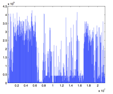
Figure 1. Think Times - the entire data set

Clearly, the nature of this data set changes over time, and the nature of truncation of heavy tails may potentially change as well. In order to study this effect we have, somewhat arbitrarily, broken the data set into four pieces, with corresponding ranges $\bigl{[}0.11\times 10^{7},0.64\times 10^{7}\bigr{]}$; $\bigl{[}0.8\times 10^{7},1.6\times 10^{7}\bigr{]}$; $\bigl{[}1.7\times 10^{7},1.9\times 10^{7}\bigr{]}$ and $\bigl{[}1.95\times 10^{7},2.1\times 10^{7}\bigr{]}$. The individual pieces are plotted on Figure 2

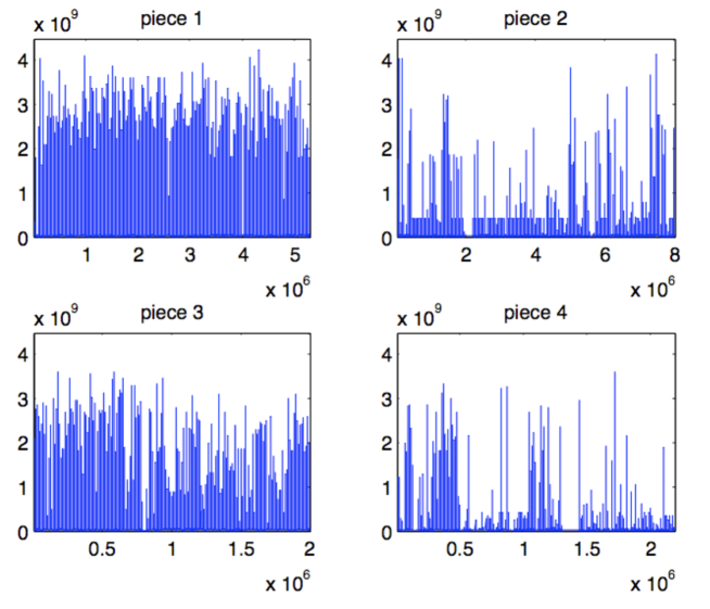
Figure 2. Think Times - the different pieces

The structure of the 4 individual pieces appears to be more stable than that of the entire data sets, and we proceed to analyze each piece separately. To do that, we first ran the Hill estimator with random $k$ given in (3.4) on the first half of each of the 4 pieces. The estimation was conducted using $\beta,\gamma=0.3,0.4,0.5,0.6,0.7$ and conservative upper bounds for $\alpha$ were obtained; these are presented in the following table.

piece	$A$
1	$3.02$
2	$2.30$
3	$0.85$
4	$2.24$

We then proceeded to use the second halves of each piece of the Think Times data set to test for soft and hard truncations.

Testing the hypothesis of soft truncation

The test statistic $Z_{n}(A_{1})$ of Section 4.1 was computed for various values of $A_{1}$ larger than $A$. The results are reported in the following table.

$A/A_{1}$	piece 1	piece 2	piece 3	piece 4
$0.5$	$31.43$	$5.81$	$154.05$	$3.57$
$0.6$	$51.59$	$7.99$	$205.37$	$4.72$
$0.7$	$77.39$	$10.74$	$271.27$	$6.11$
$0.8$	$108.08$	$14.20$	$361.74$	$7.81$
$0.9$	$142.78$	$18.57$	$491.31$	$9.91$
$0.95$	$161.38$	$21.16$	$576.73$	$11.13$

Comparing the resulting values of the test statistic with the corresponding quantiles (or their upper bounds) of $Z(A/A_{1})$, it is clear that the null hypothesis of soft truncation can be rejected for pieces 1 and 3 at the levels less that $0.01$, while for piece 2 the null hypothesis of soft truncation can be rejected at the level $0.025$, but not at the level $0.01$. For piece 4 we cannot reject the null hypothesis of soft truncation even at the level $0.05$. These findings are rather consistent with visual analysis of the pieces of the data set: piece 4 exhibits extremes that do not appear to be seriously truncated (one has to keep in mind that the visual analysis can easily be misleading).

Testing the hypothesis of hard truncation

The test statistic $Z_{n}(A;\gamma)$ of Section 4.2 was computed for various values of $\gamma$. The resulting $p$-values are reported in the following table.

$\gamma$	piece 1	piece 2	piece 3	piece 4
$0.1$	$0.85$	$0.72$	$0.88$	$0.33$
$0.2$	$0.83$	$0.98$	$0.38$	$0.57$
$0.3$	$0.97$	$0.99$	$0.79$	$0.68$
$0.4$	$0.94$	$0.68$	$0.39$	$0.43$
$0.5$	$0.83$	$0.63$	$0.94$	$0.47$
$0.6$	$0.97$	$0.89$	$0.83$	$0.27$
$0.7$	$0.91$	$0.88$	$0.87$	$0.40$
$0.8$	$0.64$	$0.85$	$0.80$	$0.33$
$0.9$	$0.70$	$0.37$	$0.85$	$0.40$

The hypothesis of hard truncation cannot be rejected for any of the four pieces. As expected, the $p$-values for piece 4 are lower than those for the other 3 pieces, but they are still rather high.

Testing a stronger version of the hypothesis of hard truncation

The test statistics $Z_{n}(A)$ of Section 4.3 was computed and the corresponding $p$-values calculated for various values of $\epsilon$. These are listed in the following table.

$\epsilon$	piece 1	piece 2	piece 3	piece 4
$0.1$	$1.00$	$1.00$	$1.00$	$1.00$
$0.2$	$1.00$	$1.00$	$1.00$	$1.00$
$0.3$	$1.00$	$1.00$	$1.00$	$0.91$
$0.4$	$1.00$	$0.73$	$1.00$	$0.45$

It is clear that even the stronger version of the hypothesis of hard truncation cannot be rejected.

5.2. Object Sizes

This data set contains $2.2\times 10^{7}$ observations. It is plotted in Figure 3. It does not appear that the nature of the observations changes with time, so we applied our statistical tests to the entire data set. After running the Hill estimator with random $k$ and parameters $\beta$ and $\gamma$ as above, on the first half of the data set, we obtained a conservative upper bound on the value of the tail exponent $\alpha$; this turned out to be $A=1.69$. We used the second half of the Object Sizes data set to test for soft and hard truncations.

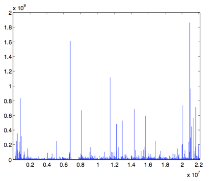
Figure 3. Data on Object Sizes

Testing the hypothesis of soft truncation

We evaluated the test statistic $Z_{n}(A_{1})$ of Section 4.1 for a range of values of $A_{1}$ larger than $A$. The results are reported in the following table.

$A/A_{1}$	$Z_{n}(A_{1})$
$0.5$	$1.75$
$0.6$	$2.32$
$0.7$	$3.09$
$0.8$	$4.10$
$0.9$	$5.42$
$0.95$	$6.23$

Comparing these with the corresponding quantiles (or their upper bounds) of $Z(A/A_{1})$, we see that the hypothesis of soft truncation cannot be rejected.

Testing the hypothesis of hard truncation

We evaluated the test statistic $Z_{n}(A;\gamma)$ of Section 4.2 for various values of $\gamma$, and the obtained $p$-values are reported in the following table.

$\gamma$	$p$-value
$0.1$	$0.50$
$0.2$	$0.36$
$0.3$	$0.73$
$0.4$	$0.77$
$0.5$	$0.95$
$0.6$	$0.94$
$0.7$	$0.94$
$0.8$	$0.97$
$0.9$	$0.72$

The null hypothesis of hard truncation cannot be rejected.

Testing a stronger version of the hypothesis of hard truncation

We calculated the test statistics $Z_{n}(A)$ of Section 4.3 for various values of $\epsilon$, and the $p$-values are given in the following table.

$\epsilon$	$p$-value
$0.1$	$1.00$
$0.2$	$0.86$
$0.3$	$0.33$
$0.4$	$0.08$

The strengthened hypothesis of hard truncation becomes suspicious for $\epsilon=0.4$, but overall our statistical tests do not produce clear evidence of the level of truncation for the Object Sizes data set.

Summary  The results of this section, especially the lack of conclusion in a number of cases, point to some of the directions for future statistical work with truncated heavy tails.

• More powerful tests are needed, together with estimates of their actual power.

• What sample sizes are necessary for the asymptotic significance levels to be applicable?

• The tests of Section 4 depend on tuning parameters $A$ and $\gamma$. At present we do not have a clear picture of the role of these parameters, or how to select them in the “optimal” way.

• What is the best way to select the parameters $\beta$ and $\gamma$ in the sample-based number of the upper order statistics in (3.4) to use in Hill estimation? Can one combine estimation of the tail index with the testing for a truncation regime in a single procedure?

6. Acknowledgment

The authors wish to thank Dr. F. Donelson Smith of the Network Research Laboratory in the Computer Science Department at the University of North Carolina at Chapel Hill for kindly providing the data sets analyzed in Section 5.

References

• Aban et al., (2006) Aban, I., Meerschaert, M., and Panorska, A. (2006). Parameter estimation for the truncated Pareto distribution. Journal of the American Statistical Association, 101(473):270–277.
• Araujo and Giné, (1980) Araujo, A. and Giné, E. (1980). The Central Limit Theorem for Real and Banach Valued Random Variables. Wiley, New York.
• Asmussen and Pihlsgard, (2005) Asmussen, S. and Pihlsgard, M. (2005). Performance analysis with truncated heavy-tailed distributions. Methodology and Computing in Applied Probability, 7(4):439–457.
• Barthelemy et al., (2008) Barthelemy, P., Bertolotti, J., and Wiersma, S. (2008). A Lévy flight for light. Nature, 453:495–498.
• Bartumeus et al., (2005) Bartumeus, F., da Luz, M., Vishwanathan, G., and Catalan, J. (2005). Animal search strategies: a quantitative random walk analysis. Ecology, 86(11):3078–3087.
• Beirlant and Guillou, (2001) Beirlant, J. and Guillou, A. (2001). Pareto index estimation under moderate right censoring. Scandinavian Actuarial Journal, 15(2):111–125.
• Beirlant et al., (2007) Beirlant, J., Guillou, A., Dieckx, G., and Fils-Villetard, A. (2007). Estimation of the extreme value index and extreme quantiles under random censoring. Extremes, 10(3):151–174.
• Billingsley, (1968) Billingsley, P. (1968). Convergence of Probability Measures. Wiley, New York.
• Brockmann et al., (2006) Brockmann, D., Hufnagel, L., and Geisel, T. (2006). The scaling laws of human travel. Nature, 439:462–465.
• Burrooughs and Tebbens, (2001) Burrooughs, S. and Tebbens, S. (2001). Upper-truncated power laws in natural systems. Pure and Applied Geophysics, 158(4):741–757.
• Corral, (2006) Corral, A. (2006). Universal earthquake-occurence jumps, correlations with time, and anomalous diffusion. Physical Review Letters, 97(17):178501.
• Csörgo et al., (1986) Csörgo, S., Horváth, L., and Mason, D. (1986). What portion of the sample makes a partial sum asymptotically stable or normal? Probability Theory and Related Fields, 72:1–16.
• de Haan and Ferreira, (2006) de Haan, L. and Ferreira, A. (2006). Extreme Value Theory: An Introduction. Springer, New York.
• Einmahl et al., (2008) Einmahl, J., Fils-Villetard, A., and Guillou, A. (2008). Statistics of extremes under random censoring. Bernoulli, 14(1):207–227.
• Embrechts et al., (1997) Embrechts, P., Klüppelberg, C., and Mikosch, T. (1997). Modelling Extremal Events for Insurance and Finance. Springer-Verlag, Berlin.
• Feller, (1971) Feller, W. (1971). An Introduction to Probability Theory and its Applications, volume 2. Wiley, New York, 2nd edition.
• Gomez et al., (2000) Gomez, C., Selman, B., Crato, N., and Kautz, H. (2000). Heavy–tailed phenomena in satisfiability and constraint satisfaction problems. Journal of Automated Reasoning, 24(1-2):67–100.
• Gut, (2005) Gut, A. (2005). Probability: A Graduate Course. Springer.
• Hill, (1975) Hill, B. (1975). A simple general approach to inference about the tail of a distribution. Ann. Statist., 3:1163–1174.
• Hong et al., (2008) Hong, S., Rhee, I., Kim, S., Lee, K., and Chong, S. (2008). Routing performance analysis of human-driven delay tolerant networks using the truncated levy walk model. In Mobility Models ’08: Proceedings of the 1st ACM SIGMOBILE workshop on Mobility models, pages 25–32, New York. ACM.
• Hult et al., (2005) Hult, H., Lindskog, F., Mikosch, T., and Samorodnitsky, G. (2005). Functional large deviations for multivariate regularly varying random walks. Annals of Applied Probability, 15(4):2651–2680.
• Jelenković, (1999) Jelenković, P. R. (1999). Network multiplexer with truncated heavy-tailed arrival streams. INFOCOM ’99. Eighteenth Annual Joint Conference of the IEEE Computer and Communications Societies. Proceedings. IEEE, 2:625–632.
• Maruyama and Murakami, (2003) Maruyama, Y. and Murakami, J. (2003). Truncated Lévy walk of a nanocluster bound weakly to an atomically flat surface: Crossover from superdiffusion to normal diffusion. Physical Review B, 67(8):085406.
• Microsoft Knowledge Base Article 154997, (2007) Microsoft Knowledge Base Article 154997 (2007). Description of the FAT32 file system.
• Mikosch, (2009) Mikosch, T. (2009). Non-Life Insurance Mathematics: An Introduction with the Poisson Process. Springer, Berlin, 2nd edition.
• Resnick, (1987) Resnick, S. (1987). Extreme Values, Regular Variation and Point Processes. Springer-Verlag, New York.
• Resnick, (2007) Resnick, S. (2007). Heavy-Tail Phenomena : Probabilistic and Statistical Modeling. Springer, New York.
• Rosiński, (1990) Rosiński, J. (1990). On series representation of infinitely divisible random vectors. The Annals of Probability, 18:405–430.
• Rvačeva, (1962) Rvačeva, E. (1962). On domains of attraction of multi-dimensional distributions. Selected Translations in Mathematical Statistics and Probability, 2:183–205. Publisher: IMS-AMS.
• Samorodnitsky and Taqqu, (1994) Samorodnitsky, G. and Taqqu, M. (1994). Stable Non-Gaussian Random Processes. Chapman and Hall, New York.
• Sato, (1999) Sato, K. (1999). Lévy Processes and Infinitely Divisible Distributions. Cambridge University Press.
• Scholtz and Contreras, (1998) Scholtz, C. and Contreras, J. (1998). Mechanics of continental rift architecture. Geology, 26(11):967–970.
• Serrano et al., (2009) Serrano, M., Flammini, A., and Menczer, F. (2009). Beyond Zipf’s law: Modeling the structure of human language. Technical Report.
• Zaninetti and Ferraro, (2008) Zaninetti, L. and Ferraro, M. (2008). On the truncated Pareto distribution with applications. Central European Journal of Physics, 6(1):1–6.