Using Premia and Nsp for Constructing
a Risk Management Benchmark for Testing Parallel Architecture

Abstract

Financial institutions have massive computations to carry out overnight which are very CPU demanding. The challenge is to price many different products on a cluster-like architecture. We have used the Premia software to valuate the financial derivatives. In this work, we explain how Premia can be embedded into Nsp, a scientific software like Matlab, to provide a powerful tool to valuate a whole portfolio. Finally, we have integrated an MPI toolbox into Nsp to enable the use of Premia to solve a bunch of pricing problems on a cluster. This unified framework can then be used to test different parallel architectures.

00000020xx

J.Ph Chancelier, B. Lapeyre and Jérôme LelongUsing Premia and Nsp

Université Paris-Est, CERMICS, École des Ponts, 6 & 8 av. B. Pascal, 77455 Marne-la-Vallée, France

Jean-Philippe Chancelier, Université Paris-Est, CERMICS, École des Ponts, 6 & 8 av. B. Pascal, 77455 Marne-la-Vallée, France

This work was supported by the French Research Agency (ANR GCPMF)

1 Introduction: The context of risk evaluation

Banking legislation (Bale II[1][4]) imposes to financial institutions some daily evaluation of the risk they are exposed to because of their market positions. The main investment banks own very large portfolios of contingent claims (several thousands of claims, 5000 being a realistic estimation).

For a given contingent claim and model parameter set, the evaluation of the price (or other risk features such as delta, gamma, vega, …) requires a computation time which can greatly vary, from a few milliseconds (for standard options in the Black Scholes model) to dozens of minutes (for American options on a large number of underlying assets).

A model is specified by several parameters: volatility, interest rate, …and, in the context of risk evaluation, it is necessary to price the contingent claims for various values of these model parameters to measure their sensibilities to the parameters. As a consequence, a huge number of atomic computations (around $10^{6}$) is necessary to evaluate the risk of the whole portfolio. These computations must be done on a daily basis to provide an evaluation of the position of the bank to the risk control organism. They are so complex that financial institutions often need to use very large clusters with up to several thousands of nodes.

Being able to have free access to both a realistic portfolio description and some model parameters would be especially useful for benchmarking (software/hardware) parallel architectures. Unfortunately, in our knowledge, no such information exists mostly because of obvious confidentiality considerations. Moreover, the evaluation of a complex portfolio needs a lot of elaborate algorithms which are seldom freely available in a unified framework.

In this work, we propose a software architecture for constructing realistic models and portfolios based on freely available softwares: Premia, MPI and Nsp. Premia[8] will be the library used to compute financial product prices and MPI will be used to control parallelism. Finally, we use a software, with a Matlab like syntax, Nsp [2] to provide a unified access to MPI and Premia primitives. Using this unified framework, we are able to generate parametrised benchmarks, to save them and to control the parallel architecture (grids, clusters,…).

We emphasise that Nsp and some implementations of MPI are available under the GPL licence and that Premia is freely available for test and experimentation purposes. Moreover, these softwares have been successfully compiled on the most widely used operating systems (Windows, Linux, Mac OS X) and their deployment on a cluster is quite easy. Such an environment is a step to define standardised benchmarks useful for the evaluation and, we hope, the conception of parallel architectures.

2 Premia: a library for numerical computations in finance

Premia is a research software devoted to the pricing and hedging of financial derivatives (see [7] for an introduction), which is a major issue for financial institutions. The algorithms are accompanied by a solid scientific documentation. The software is developed in the framework of the MATHFI research team uniting scientists working in probability and finance from INRIA and École des Ponts.

This project keeps track of the most recent advances in the field of computational finance. It focuses on the implementation of numerical analysis techniques for both probabilistic and deterministic numerical methods. An important feature of the Premia platform is its detailed documentation which provides extended references in option pricing. Besides being a single entry point for accessible overviews and basic implementations of various numerical methods, the aim of the Premia project is to be a powerful testing platform for comparing different numerical methods.

Premia is developed in interaction with a consortium of financial institutions or departments presently composed of : Calyon, Natixis, Société Générale. The members of the consortium support the development of Premia and help to determine the directions in which the project should evolve.

Premia is a fairly complete library with regards to what is currently used in advanced finance. Obviously Premia cannot claim to be an exhaustive option pricer, but it is an easy task to add any new pricing algorithms using the Premia framework. Once done, calling the new algorithm from Nsp does not require any additional work.

In its current public release, it contains finite difference algorithms, tree methods and Monte Carlo methods for pricing and hedging European and American options on equities in several models going from the standard Black-Scholes model to more complex models such as local and stochastic volatility models and even Lévy models. Sophisticated algorithms based on quantisation techniques or Malliavin calculus for European and American options are also implemented. More recently, various interest rate and credit risk models and derivatives have been added.

3 Tools

3.1 Nsp

Nsp is a Matlab like scientific software package developed under the GPL licence. It is a high-level scripting language which gives an easy access to efficient numerical routines. It can be used either as an interactive computing environment or as a programming language. It supports imperative programming and features a dynamic typing system and automatic memory management. It contains an internal class system with simple inheritance and interface implementations, this class system is visible at the Nsp programming level but not extendable at the Nsp level. When used as an interactive computing environment, it comes with online help facilities and an easy access to GUI facilities and graphics.

A large set of libraries is available and it is moreover easy to implement new functionalities. It requires to write some wrapper code also called interfaces to give glue code between the external library and Nsp internal data. The interface mechanism can be either static or dynamic, which makes it possible to build toolboxes.

Nsp shares many paradigms with other Matlab like scientific softwares as for example: Matlab, Octave, ScilabGtk[3][5] and also with scripting languages such as Python for instance.

Two typical toolboxes were used in this work. The first one is the Nsp Premia toolbox which gives access at Nsp level to the Premia financial library. The second one is a MPI interface giving access at Nsp level to mainly all MPI-2 functions.

3.2 MPI toolbox for Nsp

Having a direct access to MPI functions within a scripting language can be very useful for many aspects. The main advantage is that it gives an easy way to get familiar with the large set of MPI functions which can be tested interactively. It also hides the tedious work of packing and unpacking complex data since a scripting language contains high level data and the packing and unpacking of such data can be hidden to the user.

Similar toolboxes are available. As for example, MPITB[6] is a toolbox initially developed by Javier Fernández Baldomero and Mancia Anguita which provides such a full MPI interface for the Matlab and Octave languages. The MPINSP toolbox follows the same philosophy and was implemented using the Nsp interface language. The Matlab version of the MPItb toolbox is implemented through wrapper code which are called mexfiles and since a mexlib interface library is available in Nsp it could have been possible to make the Matlab toolbox work in Nsp with mainly no additional work. Nevertheless, for a better efficiency and flexibility the MPINSP toolbox has been directly written using the Nsp interface API.

Now, we give some examples to highlight facilities that are given inside Nsp to access MPI primitives. It is possible to launch a master Nsp and then to spawn Nsp slaves, this is done by using the MPI_Comm_spawn primitive as shown on Fig. 1:

MPI_Init();
COMM =mpicomm_create(’SELF’);
INFO_NULL=mpiinfo_create(’NULL’);
cmd = "exec(’’src/loader.sce’’);MPI_Init();";
cmd = cmd + "parent=MPI_Comm_get_parent();";
cmd = cmd + "[NEWORLD]=MPI_Intercomm_merge(parent,1);";
nsp_exe = getenv(’SCI’)+’/bin/nsp’;
args=["-name","nsp-child","-e", cmd];
[children,errs]= MPI_Comm_spawn(nsp_exe,args,1,INFO_NULL,0,COMM);
// child will execute cmd
[NEWORLD] = MPI_Intercomm_merge (children, 0);

Figure 1: MPI primitives at Nsp level

The code given in Fig. 1 will start a new Nsp which will execute the transmitted cmd to start interacting with the master through a merged communicator. Note that the interface between Nsp and MPI does not just consist in a set of functions but also on new Nsp object devoted to MPI. For example mpicomm_create creates a new Nsp communicator object which internally contains a MPI communicator. Since starting a set of Nsp slaves is a classic task, the previous code can be written in a Nsp function NSP_spawn and it is then possible to start n slaves by the simple Nsp command

NEWORLD=NSP_spawn(n);

It is possible to transmit and receive almost all the Nsp objects using the MPI_Send_Obj and MPI_Recv_Obj Nsp functions. These two functions use the fact that almost all the Nsp objects can be serialized into a Serial object. The two functions MPI_Send_Obj and MPI_Recv_Obj use internal serialization and packing to transparently transmit Nsp Objects.

-nsp->A=list(’string’,%t,rand(4,4));
-nsp->MPI_Send_Obj(A,rank,TAG,MCW)
-nsp->B=MPI_Recv_Obj(rank,TAG,MCW)
B       =               l (3)
 (
  (1)   =               s (1x1)

    string
  (2)   =                b (1x1)

   | T |
  (3)   =               r (4x4)

   |  0.89259  0.69284  0.10172  0.85434 |
   |  0.08482  0.67768  0.63584  0.16133 |
   |  0.25667  0.42840  0.73767  0.29179 |
   |  0.65078  0.37258  0.67447  0.23511 |
 )

It gives us a very easy way to transmit a Premia problem to a Nsp slave. Moreover it is easy to transmit jobs to Nsp slaves as Nsp strings.

For standard objects such as non sparse matrices, cells, lists and hash tables it is possible to use MPI_Send directly or combined with the MPI_Pack function.

A=[%t,%f];
B={’foo’,[1:4],’bar’,rand(100,100)};
H=hash_create(A=A,B=B);
P=MPI_Pack(H,MCW),
MPI_Send(P,randk,TAG,MCW)

Receiving the transmitted packed data is also easy. A mpibuf object can be created at Nsp level with a proper size and be given to the MPI_Recv function for receiving the transmitted packed data. A call to MPI_Unpack will then recreate a Nsp object.

[stat]=MPI_Probe(-1,-1,MCW)
// size in characters
[elems]=MPI_Get_elements(stat,’’)
B=mpibuf_create(elems);  // create a receive buffer
...
stat=MPI_Recv(B,randk,TAG,MCW);
H1=MPI_Unpack(B,MCW);

Moreover, it is possible to serialize objects at Nsp level and transmit them. Note, that in that case, MPI_Recv_Obj will directly unseal the received Serial object.

-nsp->A=sparse(rand(2,2));
-nsp->S=serialize(A);
-nsp->MPI_Send_Obj(S,rank,TAG,MCW)
...
-nsp->B=MPI_Recv_Obj(rank,TAG,MCW);
-nsp->B.equal[A]
ans     =                b (1x1)

 | T |

The serialization of objects is very similar to the binary format used to save and load objects in Nsp since serialization just redirects the binary savings of objects to a string buffer. Therefore, it is possible to save a set of objects in a file and then directly load the file content in a serialized object. It gives us an efficient way of transmitting Nsp data stored in a file to MPI slaves. We illustrate in the next script the sload function :

-nsp->H.A = rand(4,5);
-nsp->H.B = rand(4,1);
-nsp->save(’/tmp/saved.bin’,H);
-nsp->S=sload(’/tmp/saved.bin’)  // we directly create a Serial object
S¯= <302-bytes>¯¯ serial
-nsp->H1=S.unserialize[];
-nsp->H1.equal[H]
ans¯=¯¯ b (1x1)

| T |

Figure 2: The sload function

We have recently introduced in Nsp the possibility to compress the serialized buffer used in serialized objects. The unserialize method can then transparently manage unserialization of compressed and non compressed Serial objects. Using this facility to test if it can improve the MPI transmission of Premia problems was not studied in this paper but it is left for future developments and tests. In some Premia problems, a large set of data contained in a file has to be embedded and transmitted with the problem, we imagine that compressed serialization could be useful in those cases. Moreover, compression, which takes most of the CPU time, can be done off line when preparing a set of problems.

-nsp->A=1:100;
-nsp->S=serialize(A)
S¯= <842-bytes>¯¯ serial
-nsp->S1=S.compress[]
S1¯= <248-bytes>¯¯ serial
-nsp->A1=S1.unserialize[];
-nsp->A1.equal[A]
ans¯=¯¯ b (1x1)

| T |

A large file called TUTORIAL.sce can be used to interactively to learn MPI in general and also its Nsp interface. This file is a simple Nsp adaptation of the excellent MPITB tutorial for Matlab [6].

3.3 Premia toolbox for Nsp

For long, the only way to use Premia was from the command line. With the growing of Premia every year, the need of a real graphical user interface has become more and more pressing. The idea of embedding the Premia library in a Matlab like scientific software has come up quite naturally. Unlike a standalone graphical user interface, embedding Premia into such a scientific software provides two ways of accessing the library either through the scripting language or using the graphical capabilities of the software (see Figure 3). The possibility of accessing the Premia functions directly at the interpreter level makes it possible to make Premia interact with other toolboxes. Since the licence of Premia gives right to freely distribute the version of Premia two year older that the current release, it was important that the scientific software used can be freely obtained and has extensive graphical feature. Nsp fulfilled all these conditions.

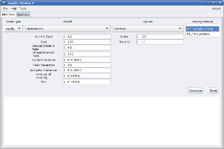
Figure 3: Premia/Nsp interface

The inheritance system of Nsp enables us to easily add new objects in the interpreter. This is how we introduced a new type named PremiaModel, through which the wide range of pricing problems described in Premia and their corresponding pricing methods are made available within Nsp. The results obtained in a given problem can be used in any post-treatment routines as any other standard data.

For practitioners, the daily valuation of complex portfolios is a burning issue to which we tried to answer using MPI/Nsp/Premia. Given a bunch of pricing problems to be solved, which are implemented in Premia, how can we make the most of Nsp and the two previously described toolboxes? First, we needed a way to describe a pricing problem in a way that is understandable by Nsp so that it can create the correct instance of the PremiaModel class. We implemented the load and save methods for such an instance relying on the XDR library (eXternal Data Representation). This way, any PremiaModel object can be saved to a file in a format which is independent of the computer architecture; these files can be reloaded later by any Nsp process. Then, a bunch of pricing problems can be represented by a list of files created either from the scripting language or using the graphical interface. Let us give an example of how to create such a file. To save the pricing of an American call option in the one dimensional Heston model using a finite difference method, one can use the following instructions

P = premia_create()
P.set_asset[str="equity"]
P.set_model[str="Heston1dim"]
P.set_option[str="PutAmer"]
P.set_method[str="MC_AM_Alfonsi_LongstaffSchwartz"]
save(’fic’, P)

Creating an instance of the PremiaModel class and setting its parameters are very intuitive. The object saved in the file fic can be reloaded using the command load(’fic’).

To solve this list of problems, we could use a single Nsp process but as the problems are totally independent it is quite natural to try to solve them in parallel using the MPI toolbox presented in Section 3.2. The master process reads all the files and creates the corresponding instances of the PremiaModel class. Then, each instance is serialized and sent to a given remote node using MPI’s communication functions.

4 Practical experiments

if ~MPI_Initialized() then   MPI_Init();end
MPI_COMM_WORLD=mpicomm_create(’WORLD’);
[mpi_rank] = MPI_Comm_rank (MPI_COMM_WORLD);¯
[mpi_size] = MPI_Comm_size (MPI_COMM_WORLD);

if mpi_rank <> 0¯¯¯¯// Slave part
  while %t then
    name = MPI_Recv_Obj(0,TAG,MPI_COMM_WORLD); // receives the name
    if name == ’’ then break; end
    [stat]=MPI_Probe(-1,-1,MPI_COMM_WORLD)
    [elems]=MPI_Get_count(stat);
    pack_obj=mpibuf_create(elems);  // creates a buffer to store the packed obejct
    stat=MPI_Recv (pack_obj, 0, TAG, MPI_COMM_WORLD); // receives the packed object
    ser_obj = MPI_Unpack (pack_obj, MPI_COMM_WORLD); // unpack
    P = unserialize(ser_obj); // unserialize
    P.compute[]; L = P.get_method_results[];
    MPI_Send_Obj(L(1)(3),0,TAG,MPI_COMM_WORLD); // sends the results back
  end
else¯¯¯¯// Master part
  Nt= size(Lpb, ’*’);
  nb_per_node = floor (Nt / (mpi_size-1));
  slv = 1;
  for pb=Lpb(1:mpi_size-1)’¯¯¯// send
    send_premia_pb (pb, slv); slv = slv + 1;
  end
  res=list();
  Lpb(1:mpi_size-1)=[];
  for pb=Lpb’
    [sl, result] = receive_res ();
    res.add_last[list(sl, result)];
    send_premia_pb (pb, sl);
  end
  for slv=1:mpi_size-1¯  // we still have mpi_size-1 receives to perform
    [sl, result] = receive_res ();
    res.add_last[list(sl, result)];
  end
  for slv=1:mpi_size-1   // tell all slaves to stop working
    MPI_Send_Obj([’’],slv,TAG,MPI_COMM_WORLD);
  end
  save(’pb-res.bin’,res);
end

Figure 4: A sample script for creating a parallel portfolio pricer

// Loads a Premia object, serializes and packs it before sending it to the
// process wih number slv
function send_premia_pb( name, slv )
  load(name);
  ser_obj = serialize (P)
  MPI_Send_Obj (name,slv,TAG,MPI_COMM_WORLD); // send name
  pack_obj = MPI_Pack (ser_obj, MPI_COMM_WORLD); // pack
  MPI_Send (pack_obj,slv,TAG,MPI_COMM_WORLD);  // send the packed object
endfunction

function [sl, result] = receive_res ()
  [stat] = MPI_Probe(-1,-1,MPI_COMM_WORLD);
  sl = stat.src;
  result = MPI_Recv_Obj(sl,TAG,MPI_COMM_WORLD);
endfunction

Figure 5: Sending a Premia object

A typical usage example of our MPI/Nsp/Premia framework is the evaluation of a large portfolio consisting of hundreds or even thousands of options. The pricing of a single option is not carried out using parallel computations but instead each option is priced on a single processor and because we have many processors at hand we can price several options simultaneously. Although load-balancing for parallel computation is a very active field of research, we have restricted to a simplified “Robbin Hood” strategy for our tests. The codes of Fig. 4 and Fig. 5 describe the load-balancing strategy used in our examples. First, the master sends one job to each slave and as soon as a slave finishes its computation and sends its answer back, it is assigned a new job. This mechanism goes on until the whole portfolio has been been treated.

We considered the examples of portfolios described in Sections 4.1, 4.2, 4.3. In Section 3.3, we explained how a pricing problem can be saved in a file relying on the XDR library, henceforth in our examples, a portfolio will be a collection of files, each file describing a precise pricing problem.

In Tables 1 and 2, the Time columns give the computation time in seconds whereas the Speedup ratio columns give the ratio $\frac{\text{CPU time for 1 CPUs}}{\text{n }\times\text{ CPU time for n CPUs}}$. When this ratio becomes close to $1$, it indicates that a linear speedup has been achieved. The columns are labelled according to the way the PremiaModel objects are passed from the master to a slave. There are three different labels : full load, NFS, serialized load. The label full load means that the master reads the content of the file describing the PremiaModel object, then creates the object, serializes it, packs it and sends it to a slave, which in turn performs the different operations the other way round to recreate the PremiaModel object. This way of transmitting objects highlights that the object created by the master would actually be useless if we could create a serialized PremiaModel object directly from the file in which it is saved. Going directly from the file to the serialized object without actually creating the object itself is precisely the purpose of the sload function (see Fig. 2 for a description of the function). This more direct way of transmitting an object is referred to by the serialized load label in the tables. The cluster on which all the tests were carried out use a NFS file system, which makes it possible for the master to only send the name of the file to be read and let the slave read the file content instead of creating the object and sending it to the slave. The use of the NFS file system is referred to by the NFS label in the different tables.

All our numerical tests were carried out on a $256-$PC cluster of SUPELEC. Each node is a dual core processor : INTEL Xeon–3075 2.66 GHz with a front side bus at 1333Mhz. The two cores of each node share 4GB of RAM and all the nodes are interconnected using a Gigabit Ethernet network. In none of the experiments, did we make the most of the dual core architecture since our code is one threaded. Hence, in our implementation a dual core processor is actually seen as two single core processors.

4.1 Premia’s regression tests

The first example we studied has been brought to our knowledge by the Premia development team which uses a bunch of non-regression tests to make sure that a change in the source code does not alter the behaviour of any algorithm. These non-regression tests consist in a single instance of any pricing problem which can be solved using Premia — a pricing problem corresponds to the choice of a model for the underlying asset, a financial product and a pricing method for computing the pricing and sometimes also the delta (first derivative of the option price with respect to the spot price). Several sets of these tests exist with different parameters and are run at least once a day. This motivated us to implement a parallel version of these non-regression tests; the speedups we managed to achieved are reported in Table 1, which shows that for a number of nodes less than $16$ we could achieve an almost linear speedup. The pricing problems are sent using the sload method but changing the way of sending problems has pretty much no effect on the computation time and speedup ratio because the communication time is negligible compared to the computation time of a single pricing problem. However, the decreasing of the speedup ratio when more than $16$ nodes are used indicates that the computation time of a single problem is too short. One way of improving the speedup ratio would be to create bunches of several pricing problems and send them all together which would considerably reduce the latency induced by communications: it is always advisable to send a single large message rather several smaller messages.

14cm

Table 1: Speedup table for the non-regression tests of Premia.

number of	Time	Speedup ratio
CPUs
2	838.004	1
4	285.356	0.9789
6	172.146	0.973597
8	124.78	0.959407
10	97.1792	0.958142
16	67.9677	0.821963
32	45.6611	0.592023
64	34.2828	0.387998
96	31.4682	0.280317
128	30.5574	0.215937
160	16.1006	0.327347
192	30.7013	0.142908
224	30.5024	0.123199
256	31.3172	0.104935

4.2 A toy portfolio for discriminating communication strategies

The purpose of this second example is to test the different ways of sending pricing problems. For this we considered a portfolio of $10,000$ vanilla options which can be priced using closed-form formula. A single price computation is then very fast and the time spent in communication is easily highlighted. From the comparison of the second and sixth columns of Tab. 2, it clearly appears that it is always better to use the sload method which consists in creating the serialized object directly from the file containing the object rather than first creating the object itself and then serializing it. The computation times obtained when relying on the NFS file system for sending the pricing problems are more difficult to analyze. Until the number of nodes used is less than $12$, the sload method performs better than the use of NFS but when the number of nodes keeps on increasing the use of the NFS file system becomes faster. One should keep in mind that the NFS file system uses a caching system which makes the following access to the same files much faster than the first one. This remark explains the huge difference in computation time between $2$ and $4$ nodes in the fourth column of Table 2. Then, the comparison with the NFS file system may be highly biased and NFS does not probably outperform the sload method so much on a clean run with a new portfolio. The only objective comparison is between the full load and serialized load, the latter is always the faster.

14cm

Table 2: Comparison of the different ways of carrying out the communications.

number of	Time	Speedup ratio	Time	Speedup ration	Time	Speedup ratio
CPUs	full load	full load	NFS	NFS	serialized load	serialized load
2	8.85665	1	16.3965	1	7.17891	1
4	3.55046	0.831503	4.91225	1.11263	1.73774	1.37706
8	3.86341	0.327492	2.52961	0.925974	1.81472	0.565132
10	4.06038	0.24236	2.08968	0.871824	1.87771	0.424802
12	3.9264	0.205061	1.77673	0.838952	1.88571	0.346091
14	3.9624	0.171937	1.57676	0.799912	1.81372	0.30447
16	4.05038	0.145775	1.40579	0.777572	1.9367	0.247118
18	3.9524	0.131813	1.27181	0.758371	1.9497	0.216591
20	4.13337	0.112775	1.17682	0.73331	1.87272	0.201759
24	3.77643	0.101967	1.02784	0.69358	1.84772	0.168925
28	3.9504	0.0830357	0.928859	0.653789	1.77273	0.149986
32	4.35934	0.0655371	0.848871	0.623086	1.83072	0.126495
36	4.05938	0.0623364	0.786881	0.595353	1.75773	0.116691
40	4.06538	0.0558604	0.832873	0.504787	1.81572	0.101378
45	4.12437	0.0488044	0.768884	0.484661	1.78273	0.0915209
50	4.19136	0.0431239	0.738887	0.452874	1.70474	0.0859417

4.3 A realistic portfolio valuation

This last example comes from the risk evaluation which every financial institution has to carry out on a daily basis. Our aim was to create a large portfolio representative of the numbers of pricing problems and of the computation cost. These portfolios are really challenging for parallel computations because the time needed to compute a single price varies a lot between the different financial derivatives composing the portfolio.

Portfolio description.

We tried to accurately reproduce the daily computation load every bank has to face for the evaluation of its risk exposure. Even though, Premia is able to price derivatives on many different kinds of underlying assets such as interest rates, commodities, credits or even inflation, we have restricted to equity derivatives for our tests. We built a portfolio of $7931$ contingent claims on stocks.

Among the equity derivatives, the easiest to price are the so–called plain vanilla options which are European call or put options in the Black & Scholes model; closed-form formulas are available for their evaluations. Our portfolio contains $1952$ such call options with maturities quarterly distributed between $4$ months and $8$ years and strikes uniformly varying between $70\%$ and $130\%$ of the spot price with a step of $1\%$.

Some options such as barrier options are more complex to price and partial differential equation techniques are often used. Even though closed-form formula for their prices do exist in the Black & Scholes model, they cannot be extended to more complex models whereas partial differential equation (PDE) techniques are more widely applicable. We consider in our portfolio $1952$ down and out call options with maturities and strikes varying as in the previous example. Because of the barrier clause in the option, the PDE must be solved with a very thin time step, namely one time step every $2$ days.

So far, we have only considered one dimensional products but many of them involve as many underlying assets as $40$ (as for the Cac 40 index). These high dimensional products are very hard to price and one has to resort to Monte–Carlo techniques to evaluate these derivatives. We usually use $10^{6}$ samples for the Monte–Carlo simulations. We have included $525$ put options on a $40$ dimensional basket with regularly distributed maturities between $0.2$ and $5$ years with a step of $0.2$ year and strikes uniformly varying between $90\%$ and $110\%$ of the spot price with a step of $1\%$.

Practitioners sometimes feel the need of using little more sophisticated models : the local volatility models which are very close to the Black & Scholes model but in which the volatility is not constant anymore but rather depends on the current time and stock price. In these models, there are no closed-form formula anymore and Monte-Carlo methods are used instead. We add $1025$ call options in a local volatility model to our portfolio. The strikes vary from $80\%$ to $120\%$ of the spot price and the maturities are regularly distributed between $0.2$ and $5$ years with a step of $0.2$ year.

Finally, some options can be exercised at any time between the emission time and a fixed time horizon : these options are called American options and can only be priced using American Monte–Carlo algorithms or PDE techniques. Both approaches are computationally very demanding. We added to our portfolio $1952$ American put options priced using PDE with the same parameters as for the plain vanilla options. The rest of the portfolio is composed of $7$ dimensional American put options with regularly distributed maturities between $0.2$ and $5$ years with a step of $0.2$ year and strikes uniformly varying between $90\%$ and $110\%$ of the spot price with a step of $1\%$. These options are priced using American Monte–Carlo techniques.

To give an insight of the computational costs for each type of options, one should keep in mind that the pricing of plain vanilla options is almost instantaneous; the Monte–Carlo and PDE approaches for European options roughly demand the same amount of computations (between $10$ and $30$ seconds); the evaluation of American products is much longer than any other (above $60$ seconds).

Experimental performances.

The computation times needed to price the whole portfolio are fairly the same no matter how the objects are sent by the master process, see Tab. 3. Even a naive load balancing as the one described in Fig. 4 enables to achieve very good speedup ratios; with $256$ nodes, the speedup ratio is still better than $0.8$. However, still increasing the number of nodes does not reduce the computation time accordingly because the average cost of a single pricing problem is too small compared to the time spent in communications. Therefore, many nodes are waiting for some more work to do, which diminishes the speedup ratio.

13.5cm

Table 3: Comparison of the different ways of carrying out the communications.

number of	Time	Speedup ratio	Time	Speedup ratio	Time	Speedup ratio
CPUs	full load	full load	NFS	NFS	serialized load	serialized load
2	5770.16	1	5799.66	1	5776.33	1
4	1980.35	0.971238	1939.46	0.996783	1925.29	1.00008
6	1154.05	0.999983	1161.25	0.998865	1157.22	0.998313
8	823.056	1.00152	828.07	1.00055	840.403	0.981897
10	641.166	0.999943	645.544	0.998239	641.096	1.00112
16	389.295	0.988139	389.097	0.993696	386.745	0.995716
32	187.441	0.993031	193.937	0.964676	189.354	0.984045
64	93.2008	0.982715	100.384	0.917062	94.7316	0.967868
96	61.5176	0.987335	69.7884	0.874774	63.1974	0.962119
128	46.7399	0.972068	54.8667	0.83232	47.6968	0.953585
160	38.4812	0.943068	41.9726	0.869039	41.1997	0.88178
192	31.5312	0.958107	35.7536	0.849278	33.5979	0.900132
224	27.2929	0.948056	31.3362	0.829948	31.5822	0.820171
256	24.4743	0.924566	28.2047	0.806382	27.8228	0.814163
320	26.1740	0.6911			26.7879	0.6760
384	20.0550	0.7512			22.5696	0.6682
512	19.7960	0.5704			20.1779	0.5602

5 Conclusion

In this work, we explained how we could use Nsp with the MPI and Premia toolboxes to address the difficult problem of parallelizing the evaluation of a large portfolio. The use of Nsp makes the parallelization very easy as all the code can be written in an intuitive scripting language. For our examples, we chose a simplified Robbin Hood approach as far as load–balancing is concerned and it already provides very good speedups. One way of improving the speedups would be to improve the load balancing mechanism. The first idea is to gather several pricing problems and send them all together to reduce the communication latency. The bottleneck in the approach we used is that the computation assigned to the first slave process is finished before the master has already assigned the last slave a job. As we do not know how long a computation will last, we cannot reorganize the works so that not all the light works are assigned to the same CPUs. Nevertheless, one way of encompassing this difficulty is to divide the nodes into sub-groups, each group having its own master. Then, each sub–master could apply a naive load balancing but since it has fewer slave processes to monitor the speedups would be better.

References

- [1] Basel II: Revised international capital framework. http://www.bis.org/bcbs.
- [2] Nsp. http://cermics.enpc.fr/~jpc/nsp-tiddly/mine.html.
- [3] ScilabGtk: a Gtk+ version of Scilab. http://www.scilabgtk.org.
- [4] Basel Committee on Banking Supervision. International convergence of capital measurement and capital standards. Technical report, Bank for International Settlements, 2006.
- [5] S. Campbell, J.-P. Chancelier, and R. Nikoukhah. Modeling and Simulation in Scilab/Scicos. 2006. ISBN: 978-0-387-27802-5.
- [6] Javier Fernández Baldomero and Mancia Anguita. MPI toolbox (mpitb). Technical report, Depto. de Arquitectura y Tecnología de Computadores, ETSI Informática, Universidad de Granada, 2000–2008. http://atc.ugr.es/javier-bin/mpitb.
- [7] D. Lamberton and B. Lapeyre. Introduction to stochastic calculus applied to finance. Chapman & Hall/CRC Financial Mathematics Series. Chapman & Hall/CRC, Boca Raton, FL, second edition, 2008.
- [8] MathFi Research Group. A platform for pricing financial derivatives. Technical report, Inria and Université Paris Est, CERMICS, École de Ponts, 2008. http://www-rocq.inria.fr/mathfi/Premia.