Detection of an anomalous cluster in a network

Abstract

We consider the problem of detecting whether or not, in a given sensor network, there is a cluster of sensors which exhibit an “unusual behavior.” Formally, suppose we are given a set of nodes and attach a random variable to each node. We observe a realization of this process and want to decide between the following two hypotheses: under the null, the variables are i.i.d. standard normal; under the alternative, there is a cluster of variables that are i.i.d. normal with positive mean and unit variance, while the rest are i.i.d. standard normal. We also address surveillance settings where each sensor in the network collects information over time. The resulting model is similar, now with a time series attached to each node. We again observe the process over time and want to decide between the null, where all the variables are i.i.d. standard normal, and the alternative, where there is an emerging cluster of i.i.d. normal variables with positive mean and unit variance. The growth models used to represent the emerging cluster are quite general and, in particular, include cellular automata used in modeling epidemics. In both settings, we consider classes of clusters that are quite general, for which we obtain a lower bound on their respective minimax detection rate and show that some form of scan statistic, by far the most popular method in practice, achieves that same rate to within a logarithmic factor. Our results are not limited to the normal location model, but generalize to any one-parameter exponential family when the anomalous clusters are large enough.

T1Supported in part by NSF Grant DMS-06-03890 and ONR Grant N00014-09-1-0258.

, and

1 Introduction

We discuss the problem of detecting whether or not, in a given network, there is a cluster of nodes which exhibit an “unusual behavior.” Suppose that we are given a set of nodes with a random variable attached to each node. We observe a realization of this process and would like to tell whether all the variables at the nodes have the same behavior, in the sense that they are all sampled from a common distribution, or whether there is a cluster of nodes at which the variables have a different distribution.

1.1 A wide array of applications

The task of detection in networks is critical for an increasing number of applications, for example, in surveillance and environment monitoring. We describe a few of these applications below.

Detection in sensor networks

The advent of sensor networks overviewsensor , 1024422 , zhao2004wireless has multiplied the amount of data and the variety of applications where the task of detection is central. Surveillance and environment monitoring are prime areas of application for sensor networks. Take, for example, the transport of hazardous materials. Currently, some major traffic bottlenecks (e.g., airports, subways and borders) use portal monitoring systems fitch2003tcr , 1352095 . Sensor networks offer a more flexible, decentralized alternative and are considered for the detection of radioactive, biological or chemical materials hills2001sd , radiation , cui2001nnh . Sensor networks are also extensively used in other target tracking settings linesand , targetsensor .

Detection in digital signals and images

A digital camera may be seen as a sensor network, with CCD or CMOS pixel sensors. As imaging systems have been available for quite some time, the literature on detection in images is quite extensive, spanning several decades, particularly in satellite imagery roadtracking , artificialnatural , shipdetection , firedetection , computer vision eyedetection , objecttracking and medical imaging medicalsurvey , breasttumor , braintumor , braams1995detection .

Disease outbreak detection

The presence of a biological or chemical material in a given geographical region may also be detected indirectly through its impact on human health. In this context, early detection of the disease outbreak is crucial in order to minimize the severity of the epidemic. For that purpose, some specific information networks are used, with surveillance systems now incorporating data from hospital emergency visits, ambulance dispatch calls and pharmacy sales of over-the-counter drugs rotz2004advances , heffernan2004ssp , wagner2001esv .

Virus detection in a computer network

Diseases affect computers as well, in the form of viruses and worms spreading from host to host in a computer network szor2005acv . Affected machines may exhibit slightly anomalous behavior (e.g., a loss of performance or violations of specific rules) which may be hard to detect on an individual machine.

Detection from field measurements

In waterquality , the water quality in a network of streams in Pennsylvania is assessed by field biologists performing a variety of analyses at various locations along the streams; the objective is to determine whether there are regions of low biological integrity based on the collected data, and to identify these regions. Other field measurements include census data and surveys involving geographical location.

Detection is, of course, closely related to estimation (i.e., the localization or extraction of the anomalous cluster of nodes), but different. This distinction is rarely made clear, however. Indeed, reliable detection is possible at lower signal-to-noise ratios than reliable estimation and it may be important to detect the presence of signals from noisy data without being able to estimate them. For example, one could imagine developing a surveillance system performing detection at relatively low energy/bandwidth costs, yet efficient at low signal-to-noise ratios, and then switching to estimation mode whenever the presence of a signal is detected. Another example would be a low cost preliminary survey involving fewer field measurements, with findings subsequently confirmed by a larger, more expensive survey.

1.2 Mathematical framework

1.2.1 Purely spatial model

We loosely model a network with a set of $m$ nodes, denoted by $\mathbb{V}_{m}$. In our examples, we will either assume that $\mathbb{V}_{m}$ is embedded in a Euclidean space or we will equip $\mathbb{V}_{m}$ with a graph structure. Our analysis is in the setting of large networks, that is, $m\to\infty$. To each node $v\in\mathbb{V}_{m}$, we attach a random variable $X_{v}$. The nodes represent the sources of information (e.g., sensors) and the variables represent the data they collect. In some settings, the data collected by each unit is multidimensional, in which case $X_{v}$ is a random vector. Our discussion readily generalizes to that setting.

The random variables are assumed to be independent. For concreteness, we consider a normal location model, popular in signal and image processing, to model the noise. Our analysis, however, generalizes to any exponential family under some conditions on the sizes of the anomalous clusters, such as Bernoulli models which arise in sensor arrays where each sensor collects one bit (i.e., makes a binary decision) or Poisson models which come up with count data, for instance, arising in infectious disease surveillance systems Kul . The extension to exponential families is detailed in Section 4.1.

The situation where no signal is present, that is, “business as usual,” is modeled as

$$\mathrm{H}_{0}^{m}\dvtx X_{v}\sim\mathcal{N}(0,1)\qquad\forall v\in\mathbb{V}_{m}.$$

Let $K$ be a cluster, which we define for now as a subset of nodes, that is, $K\subset\mathbb{V}_{m}$. In fact, we will be interested in classes of clusters that are either derived from a geometric shape, when $\mathbb{V}_{m}$ is embedded in Euclidean space, or connected components, when $\mathbb{V}_{m}$ has a graph structure. The situation where the nodes in $K$ behave anomalously is modeled as

$$\mathrm{H}_{1,K}^{m}\dvtx X_{v}\sim\mathcal{N}(\mu_{K},1)\qquad\forall v\in K;\qquad X_{v}\sim\mathcal{N}(0,1)\qquad\forall v\notin K,$$

where $\mu_{K}>0$. We choose to decompose $\mu_{K}$ as $\mu_{K}=|K|^{-1/2}\Lambda_{K}$, where $|K|$ denotes the number of nodes in $K$ and $\Lambda_{K}$ is the signal strength. Indeed, with this normalization, for any cluster $K$,

$$\min_{T}\mathbb{P}(T=1|\mathrm{H}_{0}^{m})+\mathbb{P}(T=0|\mathrm{H}_{1,K}^{m})=2\mathbb{P}\bigl{(}\mathcal{N}(0,1)>\Lambda_{K}/2\bigr{)},$$ (1)

where the minimum is over all tests for $\mathrm{H}_{0}^{m}$ versus $\mathrm{H}_{1,K}^{m}$ and the lower bound is achieved by the likelihood ratio (Neyman–Pearson) test. We define

$$\overline{\Lambda}_{m}=\max_{K\in\mathcal{K}_{m}}\Lambda_{K},\qquad\underline{\Lambda}_{m}=\min_{K\in\mathcal{K}_{m}}\Lambda_{K}.$$

Figures 1–4 illustrate the setting for various types of clusters.

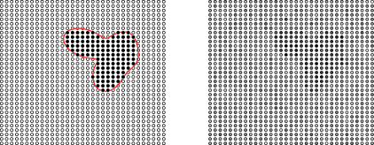
Figure 1: Left: a thick cluster is defined as the nodes within a closed curve, which is a mild deformation of a circle. Right: corresponding noisy data.

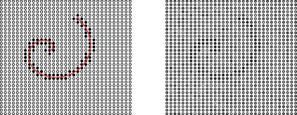
Figure 2: Left: a thin cluster is defined as the nodes within a band around a given curve. Right: corresponding noisy data.

Let $\mathcal{K}_{m}$ be a class of clusters within $\mathbb{V}_{m}$ and define

$$\mathrm{H}_{1}^{m}=\bigcup_{K\in\mathcal{K}_{m}}\mathrm{H}_{1,K}^{m}.$$

We are interested in testing $\mathrm{H}_{0}^{m}$ versus $\mathrm{H}_{1}^{m}$. In other words, under the alternative, the cluster of anomalous nodes is only known to belong to $\mathcal{K}_{m}$. We adopt a minimax point of view. For a test $T$, we define its worst-case risk as

$$\gamma_{\mathcal{K}_{m}}(T)=\mathbb{P}(T=1|\mathrm{H}_{0}^{m})+\max_{K\in\mathcal{K}_{m}}\mathbb{P}(T=0|\mathrm{H}_{1,K}^{m}).$$

The minimax risk for $\mathrm{H}_{0}^{m}$ versus $\mathrm{H}_{1}^{m}$ is defined as

$$\gamma_{\mathcal{K}_{m}}=\inf_{T}\gamma_{\mathcal{K}_{m}}(T).$$

We say that $\mathrm{H}_{0}^{m}$ and $\mathrm{H}_{1}^{m}$ are asymptotically inseparable (in the minimax sense) if

$$\mathop{\underline{\lim}}_{m\to\infty}\gamma_{\mathcal{K}_{m}}=1,$$

which is equivalent to saying that, as $m$ becomes large, no test can perform substantially better than random guessing, without even looking at the data. A sequence of tests $(T_{m})$ is said to asymptotically separate $\mathrm{H}_{0}^{m}$ and $\mathrm{H}_{1}^{m}$ if

$$\lim_{m\to\infty}\gamma_{\mathcal{K}_{m}}(T_{m})=0,$$

and $\mathrm{H}_{0}^{m}$ and $\mathrm{H}_{1}^{m}$ are said to be asymptotically separable if there is such a sequence of tests. For example, in view of (1), for any sequence of clusters $K_{m}\subset\mathbb{V}_{m}$, $\mathrm{H}_{0}^{m}$ and $\mathrm{H}_{1,K_{m}}^{m}$ are asymptotically inseparable if $\Lambda_{K_{m}}\to 0$ and they are asymptotically separable if $\Lambda_{K_{m}}\to\infty$. For convenience, we assume that no cluster in the class $\mathcal{K}_{m}$ is of size comparable to that of the entire network, that is, $\max\{|K|\dvtx K\in\mathcal{K}_{m}\}=o(m)$. This simplifies the statement of our results and detecting such clusters can easily be achieved using the test that rejects for large values of $\sum_{v\in\mathbb{V}_{m}}X_{v}$.

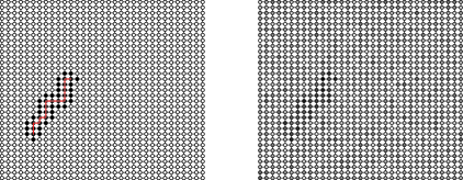
Figure 3: Left: a band defined around a path. Right: corresponding noisy data.

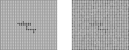
Figure 4: Left: an arbitrary connected component. Right: corresponding noisy data.

The situation we just described is purely spatial and relevant in some applications not involving time. Such situations are common in image processing. In other applications, especially in surveillance, time is an intrinsic part of the setting. In the following section, we modify the model above to incorporate time.

1.2.2 Spatio-temporal model

Building on the framework introduced in the previous section, we assume that each $X_{v}$ is now a (discrete) time series, $(X_{v}(t),t\in\mathbb{T}_{m})$, where $\mathbb{T}_{m}\subset[0,\infty)$ is finite with $|\mathbb{T}_{m}|\to\infty$; let $t_{m}=\max\{t\in\mathbb{T}_{m}\}$. Let $\mathcal{K}_{m}$ be a class of cluster sequences of the form $(K_{t},t\in\mathbb{T}_{m})$ such that $K_{t}\subset\mathbb{V}_{m}$ for all $t\in\mathbb{T}_{m}$. For example, assuming that $\mathbb{V}_{m}$ is embedded in a Euclidean space, with norm denoted by $\|\cdot\|$, a space–time cylinder (e.g., one used in disease outbreak detection diseaseoutbreak ) is a cluster sequence $(K_{t},t\in\mathbb{T}_{m})$ of the form $K_{t}=\{v\in\mathbb{V}_{m}\dvtx\|v-x_{0}\|\leq r_{0}\}$ if $t\geq t_{0}$, and $K_{t}=\varnothing$ otherwise, so that $t_{0}$ is the origin of the cluster in time and $x_{0}$ its center. Note that the radius remains constant here. Another example is that of a space–time cone, of the form $K_{t}=\{v\in\mathbb{V}_{m}\dvtx\|v-x_{0}\|\leq C(t-t_{0})\}$ if $t\geq t_{0},$ and $K_{t}=\varnothing$ otherwise, so that $(x_{0},t_{0})$ is the origin of the cluster in space–time. The random variables $\{X_{v}(t)\dvtx v\in\mathbb{V}_{m},t\in\mathbb{T}_{m}\}$ are assumed to be independent. This spatio-temporal setting is a special case of the purely spatial setting with the set of nodes $\mathbb{V}_{m}\times\mathbb{T}_{m}$. Understood as such, we are interested in testing $\mathrm{H}_{0}^{m}$ versus $\mathrm{H}_{1}^{m}$ as before.

1.3 Structured multiple hypothesis testing

Although the detection problem formulated above seems of great practical relevance, the statistics literature is almost silent on the subject, with the notable exception of the closely related topics of change-point analysis brodsky1993nmc and sequential analysis MR799155 . Indeed, the former is a special case of the spatial setting with the one-dimensional lattice, while the latter is a special case of the spatio-temporal setting where $\mathbb{V}_{m}$ has only one node. In our context, these two settings are actually equivalent.

What is further puzzling is that a number of publications addressing the task of detection in sensor networks all assume overly simplistic models. For example, in decentralized , energydriven , hierarchicalcensoring , optimaldistributed , cooperate , MR2450850 , the values at the sensors are assumed to all have the same distribution under the null and the alternative. That is, either all of the nodes are all right or they are all anomalous—in our notation, $\mathcal{K}_{m}=\{\mathbb{V}_{m}\}$. First, this is not a subtle statistical problem since, in such circumstances, it suffices to apply the optimal likelihood ratio test. Second, this assumption does not make sense in all of the applications described above, where the event to be detected is expected to only affect a small fraction of locations in the network.

In stark contrast, in all of the applications described earlier, the set of alternatives is composite. Viewing each node as performing a test of hypotheses, which is common in the literature on sensor networks, our problem falls within the framework of multiple comparisons. Multiple hypothesis testing is a rich and active line of research which is receiving a considerable amount of attention within the statistical community at the moment; see MR2387976 and references therein. The vast majority of the papers assume that the tests are independent of each other, which is clearly not the case here since, in general, the class contains clusters that intersect. This is particularly true in engineering applications, although this assumption is often made MR2213561 , MR926001 , MR1951265 .

1.4 The scan statistic

We will focus on the test that rejects for large values of the following version of the scan statistic:

$$\max_{K\in\mathcal{K}_{m}}\frac{1}{\sqrt{|K|}}\sum_{v\in K}X_{v}.$$ (2)

The chosen normalization is such that each term in the maximization is standard normal under the null and allows us to compare clusters of different sizes. It corresponds to the generalized likelihood ratio test in our context if $\Lambda_{K}$ is independent of $K\in\mathcal{K}_{m}$. The scan statistic was originally proposed in the context of cluster detection in point clouds glaz01 . This is the method of matched filters which is ubiquitous in problems of detection in a wide variety of fields, sometimes in the form of deformable templates in the engineering literature deformablereview , medicalsurvey or their nonparametric equivalent, active contours or snakes xu1998ssa . Note that the scan statistic is the prevalent method in disease outbreak detection, with many variations kulldorff2005stp , treebased , kulldorff2006ess , duczmal2006ess .

As advocated in MGD , we will not use the scan statistic directly in most cases, but rather restrict the scanning to a subset of $\mathcal{K}_{m}$. More precisely, we will introduce, on subsets of nodes $K,L\subset\mathbb{V}_{m}$, the metric

$$\delta(K,L)=\sqrt{2}\biggl{(}1-\frac{|K\cap L|}{\sqrt{|K||L|}}\biggr{)}^{1/2}$$ (3)

and will restrict the scanning to an $\varepsilon$-net of $\mathcal{K}_{m}$ with respect to $\delta$, that is, a subset $\{K_{j}\dvtx j\in J\}\subset\mathcal{K}_{m}$ with the property that for each $K\in\mathcal{K}_{m}$, there is a $j\in J$ such that $\delta(K,K_{j})\leq\varepsilon$. We will elaborate on this approach in the LABEL:supp. When $J$ is minimal, we call the resulting statistic an $\varepsilon$-scan statistic. The approximation precision $\varepsilon$ will be chosen appropriately, depending on the situation.

We focus on $\varepsilon$-scan statistics for two reasons. First, their performance is easier to analyze than that of the scan statistic itself; in fact, the main approach to analyzing the scan statistic, the chaining method of Dudley MR0220340 , MR2133757 , is via a properly chosen $\varepsilon$-scan statistic. Second, some of the classes we consider are rather large and we believe that it would be computationally impractical to scan through all of the clusters in the class; furthermore, our results show that, from an asymptotic standpoint, no substantial improvement would be gained by using the full scan statistic.

We also note that the tuning parameter $\varepsilon$ may be dispensed with if we scan over subsets of different sizes in a multiscale fashion and use a scale-dependent threshold.

1.5 Existing theoretical results

The vast majority of the literature assumes that the set of nodes is embedded in some Euclidean space, that is, $\mathbb{V}_{m}\subset\mathbb{R}^{d}$. This is the case when the nodes represent spatial locations, such as in most sensor networks. In this context, the cluster class $\mathcal{K}_{m}$ is often derived from a class of domains $\mathcal{A}$ in $\mathbb{R}^{d}$, in the following way:

$$\mathcal{K}_{m}=\{K=A\cap\mathbb{V}_{m}\dvtx A\in\mathcal{A}\}.$$ (4)

Most of the literature assumes that the class $\mathcal{A}$ is parametric, exemplified by deformable templates, for which theoretical results are available, especially in the case of the square lattice boxscan , MGD , morel , jiang , perone , boutsikas . In particular, with a normal location model, the scan statistic performs well, in the sense that it is asymptotically minimax; this is shown in MGD in a slightly different context tailored to image processing applications. We also mention the recent work HJ09 , which considers the detection of multiple clusters (intervals) of various amplitudes in the one-dimensional lattice. As for nonparametric classes of domains, MGD argues that the scan statistic is asymptotically minimax for the case of star-shaped clusters with smooth boundaries.

When $\mathbb{V}_{m}$ is endowed with a graph structure, maze considers paths of a certain length. In this setting, the scan statistic is shown to be asymptotically minimax when the graph $\mathbb{V}_{m}$ is a complete, regular tree and near-minimax for many other types of graphs, such as the $d$-dimensional lattice for $d\geq 3$. Addario-Berry et al. lugosi considers the same general testing problem with a focus on cluster classes defined within the complete graph, such as cliques and spanning trees. Note that part of the material presented here appeared in isicluster .

1.6 New theoretical results

We describe here in an informal way the results we obtain.

In Section 2, we focus on situations where the vertex set $\mathbb{V}_{m}$ is embedded in a Euclidean space and well spread out in a compact domain. Within this framework, we consider in Section 2.1 a geometric class of clusters obtained as in (4) with $\mathcal{A}$ a class of blobs that are mild deformations of the unit ball. The clusters obtained in this way are “thick,” in the sense that they are not filamentary. See Figure 1. In particular, this class contains all the common parametric classes obtained from parametric shapes such as hyperrectangles and ellipsoids, as long as the shape is not too narrow. Note that the size, the (exact) shape and the spatial location of the anomalous cluster under the alternative is unknown. In Corollary 1, we show that (under specific conditions) $\mathrm{H}_{0}^{m}$ and $\mathrm{H}_{1}^{m}$ are asymptotically inseparable if there is $\eta_{m}\to 0$ slowly enough such that, for all $K\in\mathcal{K}_{m}$,

$$\Lambda_{K}\leq(1-\eta_{m})\sqrt{2\log(m/|K|)};$$

and conversely, we show that a version of the scan statistic asymptotically separates $\mathrm{H}_{0}^{m}$ and $\mathrm{H}_{1}^{m}$ if there is $\eta_{m}\to 0$ slowly enough such that, for all $K\in\mathcal{K}_{m}$,

$$\Lambda_{K}\geq(1+\eta_{m})\sqrt{2\log(m/|K|)}.$$

Note that the detection rate is the same as for the class of balls so that, perhaps surprisingly, scanning for the location (and not the shape) is what drives the minimax detection risk.

In Section 2.2, we consider “thin” clusters, obtained as in (4) with $\mathcal{A}$ a class of “bands” around smooth curves, surfaces or higher-dimensional submanifolds. In particular, this class contains hyperrectangles and ellipsoids that are sufficiently thin; see Figure 2. It turns out that, contrary to what happens for thick clusters, scanning for the actual shape impacts the minimax detection risk and is, in fact, the main contributor for some nonparametric classes. The situation is mathematically more challenging, yet we are able to prove the following in Proposition 3. Consider the class of bands of thickness $r_{m}$ around $C^{2}$ curves of bounded curvature. Then (under specific conditions), $\mathrm{H}_{0}^{m}$ and $\mathrm{H}_{1}^{m}$ are asymptotically inseparable if

$$\overline{\Lambda}_{m}r_{m}^{1/4}(\log m)^{3/2}\to 0.$$

In Theorem 2, we show that, in the same setting, some $\varepsilon_{m}$-scan statistic asymptotically separates $\mathrm{H}_{0}^{m}$ and $\mathrm{H}_{1}^{m}$ if

$$\underline{\Lambda}_{m}r_{m}^{1/4}\to\infty.$$

Hence, some form of scan statistics achieves a detection rate within a factor of $(\log m)^{3/2}$ from the minimax rate.

In Section 2.3, we consider the spatio-temporal setting. We first consider cluster sequences that admit a “thick” limit. Cellular automata, which have been used to model epidemics MR1683061 , satisfy this condition in some cases. In Proposition 5, we show that scanning over space–time cylinders, as done in disease outbreak detection, achieves the asymptotic minimax risk. We then consider cluster sequences with controlled space–time variations, which may be a relevant model for applications such as target tracking targetsensor . We consider a fairly general model in Proposition 7.

In Section 3, we assume that $\mathbb{V}_{m}=\{0,1,\ldots,m^{1/d}-1\}^{d}$, with $m^{1/d}$ an integer, seen as a subgraph of the $d$-dimensional lattice. We first consider, in Section 3.1, bands around nearest-neighbor paths; see Figure 3. We extend the results obtained in maze to paths. For example, consider bands of thickness $h_{m}$ around a path of length $\ell_{m}$, both powers of $m$. The bounds in Theorem 3 imply that $\mathrm{H}_{0}^{m}$ and $\mathrm{H}_{1}^{m}$ are asymptotically inseparable if

$$\overline{\Lambda}_{m}(\ell_{m}/h_{m})^{-1/2}(\log m)^{3/2}\to 0.$$

Conversely, Proposition 8 states that an $\varepsilon$-scan statistic asymptotically separates $\mathrm{H}_{0}^{m}$ and $\mathrm{H}_{1}^{m}$ if

$$\underline{\Lambda}_{m}(\ell_{m}/h_{m})^{-1/2}\to\infty.$$

Therefore, some form of scan statistic is again within a factor of $(\log m)^{3/2}$ from optimal. In Section 3.2, we consider arbitrary connected components, constraining only the size; see Figure 4. In Proposition 9, we obtain a sharp detection rate for clusters of very small size.

1.7 Structure of the paper

We have just described the contents of Sections 2 and 3. Section 4 is our discussion section. We extend the results obtained for the normal location model to any exponential family in Section 4.1. Other extensions are described in Section 4.2. We state some open problems in Section 4.5. In Section 4.4, we briefly discuss the challenge of computing the scan statistic. The technical arguments are gathered in the LABEL:supp.

1.8 Notation

For two sequences of real numbers $(a_{m})$ and $(b_{m})$, $a_{m}\asymp b_{m}$ means that $a_{m}=O(b_{m})$ and $b_{m}=O(a_{m})$; $a_{m}\lesssim b_{m}$ means that $a_{m}\leq(1+o(1))b_{m}$. For $a,b\in\mathbb{R}$, we use $a\vee b$ (resp., $a\wedge b$) to denote $\max(a,b)$ [resp., $\min(a,b)$]. For $a\in\mathbb{R}$, let $[a]$ be the integer part of $a$; $\lfloor a\rfloor=[a]$ if $a$ is not an integer and $[a]-1$ otherwise; and $\lceil a\rceil=[a]+1$. For a set $A$, $|A|$ denotes its cardinality. Define $\log_{\dagger}(x)=\log x$ if $x\geq e$ and $=1$ otherwise. All the limits in the text are when $m\to\infty$. Throughout the paper, we use $C$ to denote a generic constant, independent of $m$, whose particular value may change with each appearance. We introduce additional notation in the text.

2 Clusters as geometric shapes in Euclidean space

We assume that the nodes are embedded in $\Omega_{d}\subset\mathbb{R}^{d}$, a compact set with nonempty interior. Let $\|\cdot\|$ denote the corresponding Euclidean norm. For $A\subset\Omega_{d}$ and $x\in\Omega_{d}$, let $\operatorname{dist}(x,A)={\inf_{y\in A}}\|x-y\|$ and for $r>0$, define

$$B(A,r)=\{x\in\mathbb{R}^{d}\dvtx\operatorname{dist}(x,A)<r\}.$$

In particular, $B(x,r)$ denotes the (open) Euclidean ball with center $x$ and radius $r$. On occasion, we will add a subscript $d$ to emphasize that this is a $d$-dimensional ball.

We consider a sequence $(\mathbb{V}_{m})$ of finite subsets of $\Omega_{d}$, of size $|\mathbb{V}_{m}|=m$, that are evenly spread out, in the following sense: there is a constant $C\geq 1$, independent of $m$ and a sequence $r_{m}^{*}\to 0$ such that

$$C^{-1}mr^{d}\leq|B(x,r)\cap\mathbb{V}_{m}|\leq Cmr^{d}\qquad\forall r\in[r_{m}^{*},1],\forall x\in\Omega_{d}.$$ (5)

In words, the number of nodes in any ball that is not too small is roughly proportional to its volume. For the regular lattice with $m$ nodes in $\Omega_{d}=[0,1]^{d}$, condition (5) is satisfied for $r_{m}^{*}>\sqrt{d}m^{-1/d}$. This is the smallest possible order of magnitude; indeed, for some constant $C>0$ and $r$ small enough, there is a set with more than $Cr^{-d}$ disjoint balls with centers in $\Omega_{d}$, and, by (5), they are all nonempty if $r\geq r_{m}^{*}$, which forces $r_{m}^{*}\geq Cm^{-1/d}$. Another example of interest is that of $\mathbb{V}_{m}$ obtained by sampling $m$ points from the uniform distribution, or any other distribution with a density with respect to the Lebesgue measure on $\Omega_{d}$, bounded away from zero and infinity; in that case, (5) is satisfied with high probability for $r_{m}^{*}\geq C(\log(m)/m)^{1/d}$ when $C$ is large enough; for an extensive treatment of this situation, see penrose , Chapter 4.

2.1 Thick clusters

In this section, we consider clusters as in (4), where $\mathcal{A}$ is a class of bi-Lipschitz deformations of the unit $d$-dimensional ball. This includes the vast majority of all the parametric clusters considered in the literature, such as hyperrectangles and ellipsoids, as long as the shape is not too narrow. Note that a slightly less general situation is briefly mentioned in MGD .

We start with a lower bound on the minimax detection rate for discrete balls of a given radius.

Proposition 1

Consider $\lambda_{m}\to 0$ such that $\lambda_{m}\geq r_{m}^{*}$ and let $\mathcal{K}_{m}$ be the class of all discrete balls of radius $\lambda_{m}$, that is,

$$\mathcal{K}_{m}=\{K=B(x,\lambda_{m})\cap\mathbb{V}_{m}\dvtx x\in\Omega_{d}\}.$$

$\mathrm{H}_{0}^{m}$ and $\mathrm{H}_{1}^{m}$ are then asymptotically inseparable if

$$\overline{\Lambda}_{m}\leq\sqrt{2d\log(1/\lambda_{m})}-\eta_{m},$$

where $\eta_{m}\to\infty$.

We now consider a much larger class of clusters and show that, nevertheless, a form of scan statistic achieves that same detection rate. For a function $f\dvtx A\subset\mathbb{R}^{p}\to\mathbb{R}^{d}$, its Lipschitz constant is defined as

$$\lambda_{f}=\sup_{x\neq y}\frac{\|f(x)-f(y)\|}{\|x-y\|}.$$

For $\kappa\geq 1$, let $\mathcal{F}_{d,d}(\kappa)$ be the subclass of bi-Lipschitz functions $f\dvtx B(0,1)\subset\mathbb{R}^{d}\to\Omega_{d}$ such that $\lambda_{f}\lambda_{f^{-1}}\leq\kappa$ or, equivalently,

$$\sup_{x\neq y}\frac{\|f(x)-f(y)\|}{\|x-y\|}\leq\kappa\inf_{x\neq y}\frac{\|f(x)-f(y)\|}{\|x-y\|}.$$ (6)

For a function $f\dvtx A\to\mathbb{R}^{d}$, define

$$K_{f}=\operatorname{im}(f)\cap\mathbb{V}_{m},\qquad\operatorname{im}(f):=\{f(x)\dvtx x\in A\}.$$

Note that $\lambda_{f}$ is intimately related to the size of $\operatorname{im}(f)$ and therefore of $K_{f}$. Indeed, a simple application of (6) implies that, for any $f\in\mathcal{F}_{d,d}(\kappa)$,

$$B\bigl{(}f(0),\lambda_{f}/\kappa\bigr{)}\subset\operatorname{im}(f)\subset B(f(0),\lambda_{f}).$$ (7)

This implies that sets of the form $\operatorname{im}(f)$, with $f\in\mathcal{F}_{d,d}(\kappa)$, are “thick,” in the sense that the smallest ball(s) containing $\operatorname{im}(f)$ and the largest ball(s) included in $\operatorname{im}(f)$ are of comparable sizes.

Theorem 1

Consider $\lambda_{m}\to 0$ such that $\lambda_{m}\geq r_{m}^{*}$ and define

$$\mathcal{K}_{m}=\{K_{f}\dvtx f\in\mathcal{F}_{d,d}(\kappa),\lambda_{f}\geq\lambda_{m}\}.$$

An $\varepsilon_{m}$-scan statistic with $\varepsilon_{m}\to 0$ and $\varepsilon_{m}(\log(1/\lambda_{m}))^{1/(2d)}\to\infty$ then asymptotically separates $\mathrm{H}_{0}^{m}$ and $\mathrm{H}_{1}^{m}$ if

$$\underline{\Lambda}_{m}\geq\sqrt{2d\log(1/\lambda_{m})}+\eta_{m},$$

where $\eta_{m}=\varepsilon_{m}^{2}\sqrt{2d\log(1/\lambda_{m})}$. Moreover, if $r_{m}^{*}\asymp m^{-1/d}$ and

$$\mathcal{K}_{m}=\{K_{f}\dvtx f\in\mathcal{F}_{d,d}(\kappa)\},$$

then an $\varepsilon_{m}$-scan statistic with $\varepsilon_{m}\to 0$ and $\varepsilon_{m}(\log m)^{1/(2d)}\to\infty$ asymptotically separates $\mathrm{H}_{0}^{m}$ and $\mathrm{H}_{1}^{m}$ if

$$\underline{\Lambda}_{m}\geq\sqrt{2\log m}+\eta_{m},$$

where $\eta_{m}=\varepsilon_{m}^{2}\sqrt{2\log m}$.

Therefore, on a larger class of mild deformations of the unit ball, some form of scan statistic achieves essentially the same detection rate as for the class of balls stated in Proposition 1.

We note that the lower bound on $\underline{\Lambda}_{m}$ is driven by the smaller clusters in the class and that the performance guarantee is subject to a proper choice of $\varepsilon_{m}$. A simple fix for both issues is to combine the tests for different cluster sizes with an appropriate correction for multiple testing. We summarize the consequence of Proposition 1 and Theorem 1 with this observation in the following result, inspired by boxscan .

Corollary 1

Consider $\lambda_{m}\to 0$ such that $\lambda_{m}\geq r_{m}^{*}$ and define

$$\mathcal{K}_{m}=\{K_{f}\dvtx f\in\mathcal{F}_{d,d}(\kappa),\lambda_{m}\geq\lambda_{f}\geq r_{m}^{*}\}.$$

$\mathrm{H}_{0}^{m}$ and $\mathrm{H}_{1}^{m}$ are then asymptotically inseparable if, for all $K\in\mathcal{K}_{m}$,

$$\Lambda_{K}\leq\sqrt{2\log(m/|K|)}-\eta_{m},$$

where $\eta_{m}\to\infty$. Conversely, let $T_{\ell}$ be an $\varepsilon_{\ell}$-scan statistic for the subclass $\{K_{f}\in\mathcal{K}_{m}\dvtx 2^{-\ell}\leq\lambda_{f}<2^{-\ell+1}\}$ with $\varepsilon_{\ell}\ell^{1/(2d)}\to\infty$. There is a test based on $\{T_{\ell}\dvtx\ell\geq 0\}$ that asymptotically separates $\mathrm{H}_{0}^{m}$ and $\mathrm{H}_{1}^{m}$ if, for all $K\in\mathcal{K}_{m}$,

$$\Lambda_{K}\geq\sqrt{2\log(m/|K|)}+\eta_{K},$$

where $\eta_{K}=\varepsilon_{\ell_{K}}^{2}\sqrt{2\log(m/|K|)}$ and $\ell_{K}=\log(m/|K|)$.

The same procedure, that is, combining $\varepsilon$-scan statistics at different (dyadic) scales, may be implemented in any of the settings we consider in this paper to obtain a test that does not depend on a tuning parameter like $\varepsilon_{m}$ and achieves the same optimal rate at every size. This is simply due to the fact that we only need to consider the order of $\log m$ scales and the fast decaying tails of the scan statistics under the null.

Union of thick clusters

In a number of situations, the signal to be detected may be composed of several clusters. Our results extend readily to this case. Let $j_{m}$ be a positive integer and consider sets of the form $\bigcup_{j=1}^{j_{m}}K_{f_{j}}$, where the union is over some $f_{j}\in\mathcal{F}_{d,d}(\kappa)$ such that, for $j,j^{\prime}$, $\lambda_{f_{j}}\leq C\lambda_{f_{j^{\prime}}}$ and

$$\|f_{j}(0)-f_{j^{\prime}}(0)\|\leq C(\lambda_{f_{j}}\vee\lambda_{f_{j^{\prime}}}),$$

so that the sets $\operatorname{im}(f_{j})$ and $\operatorname{im}(f_{j^{\prime}})$ are of comparable sizes and not too far from each other. In that case, Theorem 1 applies unchanged, as long as the number of clusters is not too large, specifically if $j_{m}=o(\log(1/\lambda_{m}))^{1/d}$. (This can be improved if the $K_{f_{j}}$’s do not overlap too much.) If the proximity constraint is dropped, then the term $\log(1/\lambda_{m})$ in Theorem 1 is replaced by $j_{m}\log(1/\lambda_{m})$.

2.2 Thin clusters

In this section, we consider clusters that are built from smooth embeddings in $\Omega_{d}$ of the unit $p$-dimensional ball, where $p<d$. The special case of curves ($p=1$) is, for example, relevant in road tracking roadtracking and in modeling blood vessels in medical imaging bloodvessel04 . As in the previous section, the results we obtain below are valid for (some) unions of such subsets and, in particular, for submanifolds with a wide array of topologies.

For a differentiable function $f$ between two Euclidean spaces, let $Df$ denote its Jacobian matrix. For $\kappa\geq 1$, let $\mathcal{F}_{p,d}(\kappa)$ be the class of twice differentiable, one-to-one functions $f\dvtx B(0,1)\subset\mathbb{R}^{p}\to\operatorname{im}(f)\subset\Omega_{d}$ satisfying $\lambda_{f}\lambda_{f^{-1}}\leq\kappa$ and $\lambda_{Df}\leq\kappa\lambda_{f}$. We consider clusters that are tubular regions around the range of functions in $\mathcal{F}_{p,d}(\kappa)$. For a function $f$ with values in $\mathbb{R}^{d}$ and $r>0$, define

$$K_{f,r}=B(\operatorname{im}(f),r)\cap\mathbb{V}_{m}.$$

Again, $\lambda_{f}$ is intimately related to the size of $B(\operatorname{im}(f),r)$ and $K_{f,r}$. This relationship is made explicit in the LABEL:supp. We consider classes of clusters of the form $\{K_{f,r}\dvtx f\in\mathcal{F}\}$, where $\mathcal{F}$ is a subclass of $\mathcal{F}_{p,d}(\kappa)$.

We start with a result on the performance of the scan statistic. For a class $\mathcal{F}$ of functions with values in $\mathbb{R}^{d}$ and for $\varepsilon>0$, let $N_{\varepsilon}(\mathcal{F})$ denote its $\varepsilon$-covering number for the sup-norm, that is,

$$N_{\varepsilon}(\mathcal{F})=\min\Bigl{\{}n\dvtx\exists f_{1},\ldots,f_{n}\in\mathcal{F}\mbox{, s.t. }{\max_{f\in\mathcal{F}}\min_{j}}\|f-f_{j}\|_{\infty}\leq\varepsilon\Bigr{\}}.$$

Theorem 2

Let $C$ be the constant defined in Lemma B.2 in the reffmtLABEL:suppreffmt. Consider $\lambda_{m},r_{m}\to 0$ such that $C^{-1}\lambda_{m}\geq r_{m}\geq r_{m}^{*}$ and let $\mathcal{F}$ be a subclass of $\mathcal{F}_{p,d}(\kappa)$. Define

$$\mathcal{K}_{m}=\{K_{f,r}\dvtx f\in\mathcal{F},\lambda_{f}\geq\lambda_{m},C^{-1}\lambda_{m}\geq r\geq r_{m}\}.$$

An $\varepsilon_{m}$-scan statistic with $\varepsilon_{m}=o(r_{m}^{1/2})$ then asymptotically separates $\mathrm{H}_{0}^{m}$ and $\mathrm{H}_{1}^{m}$ if

$$\underline{\Lambda}_{m}\geq(1+\varepsilon_{m}^{2})\sqrt{2\log N_{\varepsilon_{m}^{2}}(\mathcal{F})+2d\log(1/\lambda_{m})}.$$

Just as in Theorem 1, if $r_{m}^{*}\asymp m^{-1/d}$, we can dispense with the restriction $r_{m}\geq r_{m}^{*}$ and replace the factor $\log(1/\lambda_{m}^{d})$ by $\log m$ in the bound.

For a typical parametric class $\mathcal{F}$, $\log N_{\varepsilon}(\mathcal{F})\sim a(\mathcal{F})\log(1/\varepsilon)$, so the scan statistic (over an appropriate net) is accurate if

$$\underline{\Lambda}_{m}\geq(1+r_{m})\sqrt{2a(\mathcal{F})\log(1/r_{m})+2d\log(1/\lambda_{m})}.$$ (8)

On the other hand, $\log N_{\varepsilon}(\mathcal{F})\asymp(1/\varepsilon)^{a(\mathcal{F})}$ for a typical nonparametric class $\mathcal{F}$ MR0124720 , so the scan statistic (over an appropriate net) is accurate if

$$\underline{\Lambda}_{m}r_{m}^{a(\mathcal{F})/2}\to\infty.$$ (9)

Finding a sharp lower bound for the minimax detection rate is more challenging for thin clusters compared to thick clusters. By considering disjoint tubes around $p$-dimensional hyperrectangles, we obtain a lower bound that matches, in order of magnitude, the rate achieved by the scan statistic when the class $\mathcal{F}$ is parametric, displayed in (8).

Proposition 2

Consider $\lambda_{m},r_{m}\to 0$ with $\lambda_{m}\geq r_{m}\geq r_{m}^{*}$. Let $U\dvtx\mathbb{R}^{p}\to\mathbb{R}^{d}$ be the canonical embedding so that $Ux=(x,0)$ and let

$$\mathcal{F}=\{f\dvtx B(0,1)\subset\mathbb{R}^{p}\to\Omega_{d},f(x)=\lambda_{m}Ux+b\mbox{, where }b\in\mathbb{R}^{d}\}.$$

Define

$$\mathcal{K}_{m}=\{K_{f,r_{m}}\dvtx f\in\mathcal{F}\}.$$

$\mathrm{H}_{0}^{m}$ and $\mathrm{H}_{1}^{m}$ are then asymptotically inseparable if

$$\underline{\Lambda}_{m}\leq\sqrt{2(d-p)\log(1/r_{m})+2p\log(1/\lambda_{m})}-\eta_{m},$$

where $\eta_{m}\to\infty$.

The proof is parallel to that of Proposition 1 and is therefore omitted.

For at least one family of nonparametric curves ($p=1$), we show that the rate displayed at (9) matches the minimax rate, except for a logarithmic factor. For concreteness, we assume that $\Omega_{d}=[0,1]^{d}$. Let $\mathcal{H}(\alpha,\kappa)$ be the Hölder class of functions $g\dvtx[0,1]\to[0,1]$ satisfying

$$\bigl{|}g^{(s)}(x)\bigr{|} \leq \kappa\qquad\forall x\in[0,1],\forall s<\alpha;$$

$$\bigl{|}g^{(\lfloor\alpha\rfloor)}(x)-g^{(\lfloor\alpha\rfloor)}(y)\bigr{|} \leq \kappa|x-y|^{\alpha-\lfloor\alpha\rfloor}\qquad\forall x,y\in[0,1].$$

Proposition 3

Let $r_{m}\to 0$ with $r_{m}\geq r_{m}^{*}$. Let $\mathcal{F}$ be the class of functions of the form $f(x)=(x,g_{1}(x),\ldots,g_{d-1}(x))$, where $g_{j}\in\mathcal{H}(\alpha,\kappa)$, with $\alpha\geq 2$. Define

$$\mathcal{K}_{m}=\{K_{f,r_{m}}\dvtx f\in\mathcal{F}\}.$$

$\mathrm{H}_{0}^{m}$ and $\mathrm{H}_{1}^{m}$ are then asymptotically inseparable if

$$\overline{\Lambda}_{m}r_{m}^{1/(2\alpha)}(\log m)^{3/2}\to 0.$$

Thus, for the detection of curves with Hölder regularity, a scan statistic achieves the minimax rate within a poly-logarithmic factor. We prove Proposition 3 by reducing the problem of detecting a band in a graph so that we can use results from Section 3.1. We do not know how to generalize this approach to higher-dimensional surfaces (i.e., $p\geq 2$).

2.3 The spatio-temporal setting

In this section, we consider the spatio-temporal setting described in Section 1.2.2. This is a special case of the spatial setting we have considered thus far, with time playing the role of an additional dimension. For their relevance in applications and concreteness of exposition, we focus on two specific models. In Section 2.3.1, we consider cluster sequences with a limit; as we shall see, this assumption is implicit in some popular models for epidemics. In Section 2.3.2, we consider cluster sequences of bounded variations.

In the remainder of this section, we assume, for concreteness, that $\mathbb{T}_{m}=\{0,1,\ldots,t_{m}\}$ with $t_{m}\to\infty$. Our results apply without any changes if the set of nodes varies with time, that is, with index set of the form ${\prod_{t\in\mathbb{T}_{m}}}\mathbb{V}_{m}^{t}$, in the case where each $\mathbb{V}_{m}^{t}$ satisfies (5) with $C$ and $r_{m}^{*}$ independent of $t$.

2.3.1 Cluster sequences with a limit

We focus here on cluster sequences obeying $K_{t_{m}}\neq\varnothing$, that is, the anomalous cluster is present at the last time point. This is a standing assumption in syndromic surveillance systems diseaseoutbreak . To illustrate the difference, consider a typical change-point problem setting, where $\mathbb{V}_{m}$ contains only one node and, for simplicity, assume that $\Lambda_{K}$ is independent of $K$ and that $\Lambda_{m}$ denotes this common value. First, let the cluster be any discrete interval (in time), so the signal may not be present at time $t=t_{m}$. This is a special case of Section 2.1, with time playing the role of a spatial dimension ($d=1$); we saw in Corollary 1 that the detection threshold is at $\Lambda_{m}\sim\sqrt{2\log|\mathbb{T}_{m}|}$. Now, let the emerging cluster be any discrete interval that includes $t=t_{m}$. Detecting such an interval is actually much easier since we do not need to search where the interval is located, which is what drives the detection threshold for the thick clusters in Section 2.1—we need only determine its length. Specifically, the scan statistic over the dyadic intervals containing $t=t_{m}$ asymptotically separates the hypotheses if $\Lambda_{m}\asymp\sqrt{{\log\log}|\mathbb{T}_{m}|}$.

Regarding the actual evolution of the cluster in time, a number of growth models have been suggested, for example, cellular automata MR2367301 , MR1849342 and their random equivalent, threshold growth automata MR2206346 , MR1698409 , which have been used to model epidemics MR1683061 . The latter includes the well-known Richardson model Richardson1973jk . Under some conditions, these models develop an asymptotic shape (with probability one), a convex polygon in the case of threshold growth automata. Less relevant for modeling epidemics, internal diffusion limited aggregation is another growth model with a limiting shape Lawler1992jk .

The simplest cluster sequences with limiting shape are space–time cylinders, for which we have the equivalent of Proposition 1. (The proof is completely parallel and we omit details.)

Proposition 4

Consider $\lambda_{m}\to 0$ with $\lambda_{m}\geq r_{m}^{*}$ and let $\mathcal{K}_{m}$ be the class of all space–time cylinders of the form $K_{t}=B(x,\lambda_{m})\cap\mathbb{V}_{m},\forall t=0,\ldots,t_{m}$, where $x\in\Omega_{d}$. $\mathrm{H}_{0}^{m}$ and $\mathrm{H}_{1}^{m}$ are then asymptotically inseparable if

$$\underline{\Lambda}_{m}\leq\sqrt{2d\log(1/\lambda_{m})}-\eta_{m},$$

where $\eta_{m}\to\infty$.

With only one possible shape and known starting point, such a model is rather uninteresting. We now consider a much larger class of cluster sequences with some sort of limit [in the sense of (10)] and show that, nevertheless, a form of scan statistic achieves that same detection rate. For a cluster sequence $K=(K_{t},t\in\mathbb{T}_{m})$, let $t_{K}=\min\{t\dvtx K_{t}\neq\varnothing\}$, which is the time when $K$ originates. The following is the equivalent of Theorem 1. The metric $\delta$ appearing below is defined in (3).

Proposition 5

Consider sequences $\lambda_{m}\to 0$ with $\lambda_{m}\geq r_{m}^{*}$ and $\log\log t_{m}=o(\log(1/\lambda_{m}))$, and a function $\nu(t)$ with $\lim_{t\to\infty}\nu(t)=0$ and $\nu(t)\leq 1$ for all $t\geq 0$. Let $\mathcal{K}_{m}$ be a class of cluster sequences such that $t_{m}-\max\{t_{K}\dvtx K\in\mathcal{K}_{m}\}\to\infty$ and, for each $K=(K_{t},t\in\mathbb{T}_{m})\in\mathcal{K}_{m}$, there exists $f\in\mathcal{F}_{d,d}(\kappa)$ with $\lambda_{f}\geq\lambda_{m}$ such that

$$\delta\bigl{(}K_{t},\operatorname{im}(f)\cap\mathbb{V}_{m}\bigr{)}\leq\nu(t-t_{K})\qquad\forall t\in\mathbb{T}_{m}.$$ (10)

There is then a scan statistic over a family of space–time cylinders that asymptotically separates $\mathrm{H}_{0}^{m}$ and $\mathrm{H}_{1}^{m}$ if

$$\underline{\Lambda}_{m}\geq(1+\xi_{m})\sqrt{2d\log(1/\lambda_{m})},$$

where $\xi_{m}\to 0$ slowly enough.

If the starting time is uniformly bounded away from $t_{m}$ and the convergence to the thick spatial cluster [in the sense of (10)] occurs at a uniform speed, then all of the cluster sequences in the class have sufficient time to develop into their “limiting” shapes. The space–time cylinders over which we scan are based on an $\varepsilon$-net for the possible limiting shapes, that is, the class of thick clusters.

Scanning over space–time cylinders (with balls as bases) is advocated in the disease outbreak detection literature diseaseoutbreak . Although seemingly naive, this approach achieves, in our asymptotic setting, the minimax detection rate if the cluster sequences develop into balls and, in general, falls short by a constant factor.

We mention that the equivalent of Corollary 1 holds here as well, in that we can combine the different scans at different space–time scales to obtain a test that does not depend on a tuning parameter (implicit here) and which achieves the same rate for the cluster class defined as above, but with $\lambda_{m}\geq\lambda_{f}\geq r_{m}^{*}$, which is the class that appears in Corollary 1.

2.3.2 Cluster sequences of bounded variation

In target tracking linesand , targetsensor , the target is usually assumed to be limited in its movements due to maximum speed and maneuverability. With this example in mind, we consider classes of cluster sequences of bounded variation, meaning that the cluster is limited in the amount it can change in a given period of time. As the rates we obtain in this subsection are the same with or without the condition $K_{t_{m}}\neq\varnothing$, we do not make that assumption. Let $t_{K}^{+}=\max\{t\dvtx K_{t}\neq\varnothing\}$.

We consider space–time tubes around Hölder space–time curves. For $\alpha\in(0,1]$ and $\kappa>0$, let $\mathcal{H}_{\infty}(\alpha,\kappa)$ be the Hölder class of functions $g\dvtx[0,\infty)\to[0,1]$ satisfying

$$|g(x)-g(y)|\leq\kappa|x-y|^{\alpha}\qquad\forall x,y\in[0,\infty).$$ (11)

The following is the equivalent of Proposition 3.

Proposition 6

Assume that $\Omega_{d}=[0,1]^{d}$. Consider sequences $r_{m}\to 0$ with $r_{m}\geq 2r_{m}^{*}$ and $\xi_{m}$ such that $1\leq\xi_{m}\leq t_{m}$. Let $\mathcal{K}_{m}$ be the class of all cluster sequences $K_{g}$ of the form $K_{g,t}=B(g(t/\xi_{m}),r_{m})\cap\mathbb{V}_{m}$ for all $t=t_{K},\ldots,t_{K}^{+}$, for some $g=(g_{1},\ldots,g_{d})$ with $g_{j}\in\mathcal{H}_{\infty}(\alpha,\kappa)$. Then, $\mathrm{H}_{0}^{m}$ and $\mathrm{H}_{1}^{m}$ are asymptotically inseparable if

$$\overline{\Lambda}_{m}(t_{m}/\lceil\xi_{m}r_{m}^{1/\alpha}\rceil)^{-1/2}\log(t_{m}/\lceil\xi_{m}r_{m}^{1/\alpha}\rceil)\bigl{(}\log(\xi_{m})+\log\log(t_{m})\bigr{)}^{1/2}\to 0.$$

Conversely, an $\varepsilon$-scan statistic with $\varepsilon<\sqrt{2}$ asymptotically separates $\mathrm{H}_{0}^{m}$ and $\mathrm{H}_{1}^{m}$ if

$$\underline{\Lambda}_{m}\bigl{(}(t_{m}/\lceil\xi_{m}r_{m}^{1/\alpha}\rceil)\log_{\dagger}(\xi_{m}^{-1}r_{m}^{-1/\alpha})+\log m\bigr{)}^{-1/2}\to\infty.$$

For simplicity, assume that $t_{m}$ is a power of $m$. If $\xi_{m}r_{m}^{1/\alpha}=O(1)$, then the detection threshold is roughly of order $t_{m}^{1/2}$, while if $\xi_{m}r_{m}^{1/\alpha}$ is large, yet small enough that $t_{m}/(\xi_{m}r_{m}^{1/\alpha})$ is still a power of $m$, then the detection threshold is roughly of order $(t_{m}/(\xi_{m}r_{m}^{1/\alpha}))^{1/2}$.

A form of scan statistic is actually able to attain the same detection rate when the radius is unknown, but restricted to $r\geq r_{m}$. In fact, another form of scan statistic achieves a slightly different rate over a much larger class of cluster sequences with bounded variations. Let $\mathcal{S}(r,\kappa)$ be the set of subsets $S\subset\Omega_{d}$ such that $B(x,r)\subset S\subset B(x,\kappa r)$ for some $x\in\Omega_{d}$.

Proposition 7

Consider a sequence $\xi_{m}$ such that $1\leq\xi_{m}\leq t_{m}$ and a constant $\eta>0$. Define $\mathcal{K}_{m}$ as the class of cluster sequences $K$ such that, for each $t=t_{K},\ldots,t_{K}^{+}$, $K_{t}=S_{t}\cap\mathbb{V}_{m}$, where $S_{t}\in\mathcal{S}(r_{t},\kappa)$ for some $r_{t}\geq r_{m}^{*}$, and, for any $s,t=t_{K},\ldots,t_{K}^{+}$,

$$\delta(K_{t},K_{s})\leq\eta\qquad\mbox{if }|t-s|\leq\xi_{m}.$$ (12)

Then, for $\eta$ small enough, an $\varepsilon$-scan statistic with $\varepsilon<\sqrt{2}$ asymptotically separates $\mathrm{H}_{0}^{m}$ and $\mathrm{H}_{1}^{m}$ if

$$\underline{\Lambda}_{m}\bigl{(}(t_{m}/\xi_{m})(\log m)+\log t_{m}\bigr{)}^{-1/2}\to\infty.$$

Consider the condition

$$\delta(K_{t},K_{s})\leq\nu(|t-s|/\xi_{m})\qquad\forall s,t\in\{t_{K},\ldots,t_{K}^{+}\},$$ (13)

for a function $\nu\dvtx[0,\infty)\to[0,\sqrt{2}]$. Then, (12) is satisfied with $\eta=\nu(1)$ and the same $\xi_{m}$. The requirement in Proposition 7 is that $\nu(1)$ be small enough. In particular, the cluster sequences considered in Proposition 6 satisfy, for some constant $C>0$,

$$\delta(K_{t},K_{s})\leq Cr_{m}^{-1/2}\bigl{(}r_{m}^{*}\vee(|t-s|/\xi_{m})^{\alpha}\bigr{)}^{1/2}\qquad\forall s,t\in\{t_{K},\ldots,t_{K}^{+}\}.$$

This comes from Lemma C.1 in the LABEL:supp and (11). Therefore, assuming $\xi_{m}\ll(r_{m}^{*})^{-1/\alpha}$, (13) is satisfied with $\nu(u)=u^{\alpha/2}$ and $\xi_{m}$ replaced by $\xi_{m}r_{m}^{1/\alpha}$. In that case, the detection rates obtained by the scan statistics of Propositions 6 and 7 are of comparable orders of magnitude.

3 Clusters as connected components in a graph

In this section, we model the network with the $d$-dimensional square lattice; specifically, we assume that $m^{1/d}$ is an integer (for convenience) and consider $\mathbb{V}_{m}=\{0,1,\ldots,\break m^{1/d}-1\}^{d}$, seen as a subgraph of the usual $d$-dimensional lattice. We assume that $d\geq 2$ since the case where $d=1$ is treated in Section 2.1. We work with the $\ell^{1}$-norm, which corresponds to the shortest-path distance in the graph; let $B(v,h)$ denote the corresponding open ball with center $v$ and radius $h$ so that $B(v,h)=\{v\}$ for $h\in(0,1]$, and, for a subset of nodes $V$, let $B(V,h)=\bigcup_{v\in V}B(v,h)$.

3.1 Paths and bands

A nearest-neighbor band of length $\ell$ and width $h$ is of the form $B(V,h)$, where $V=(v_{0},\ldots,v_{\ell})$ forms a path in $\mathbb{Z}^{d}$. A band with unit width ($h=1$) is just a path.

We say that a path $(v_{0},\ldots,v_{\ell})$ in ${\mathbb{Z}}^{d}$ is nondecreasing if, for all $t=1,\ldots,\ell$, $v_{t}-v_{t-1}$ has exactly one coordinate equal to 1 and all other coordinates equal to 0. The case of paths was treated in detail in maze ; it corresponds to taking $h_{m}=1$ below.

Theorem 3

Suppose that $d\geq 2$ and let $\mathcal{K}_{m}$ be the class of bands of width $h_{m}$ generated by nondecreasing paths in $\mathbb{V}_{m}$ of length $\ell_{m}$, starting at the origin, with $m^{1/d}\geq\ell_{m}\geq h_{m}$. Then, $\mathrm{H}_{0}^{m}$ and $\mathrm{H}_{1}^{m}$ are asymptotically inseparable if

$$\overline{\Lambda}_{m}(\ell_{m}/h_{m})^{-1/2}\log_{\dagger}(\ell_{m})(\log h_{m}+\log_{\dagger}\log\ell_{m})^{1/2} \to 0\qquad\mbox{for }d=2,$$

$$\overline{\Lambda}_{m}(\ell_{m}/h_{m})^{-1/2}(\log_{\dagger}h_{m})(\log_{\dagger}\log h_{m}) \to 0\qquad\mbox{for }d\geq 3.$$

Conversely, an $\varepsilon$-scan statistic with $\varepsilon<\sqrt{2}$ fixed asymptotically separates $\mathrm{H}_{0}^{m}$ and $\mathrm{H}_{1}^{m}$ if

$$\underline{\Lambda}_{m}(\ell_{m}/h_{m})^{-1/2}\to\infty.$$

For the case of nondecreasing paths, a form of the scan statistic achieves the minimax rate in dimension $d\geq 3$, while it falls short by a logarithmic factor in dimension $d=2$. In the latter setting, Arias-Castro et al. maze introduces a test that asymptotically separates $\mathrm{H}_{0}^{m}$ and $\mathrm{H}_{1}^{m}$ if

$$\underline{\Lambda}_{m}(\ell_{m}/h_{m})^{-1/2}\log_{\dagger}(\ell_{m})^{1/2}\to\infty,$$ (14)

coming slightly closer to the minimax rate.

In fact, even when the band has unknown length, width and starting location, and when the path is not restricted to be nondecreasing, a form of scan statistic achieves the same rate, except for a logarithmic factor.

Proposition 8

Suppose that $d\geq 2$ and let $\mathcal{K}_{m}$ be the class of all bands of width $h$ and length $\ell$, where $\ell_{m}\geq\ell\geq h\geq h_{m}$, that are within $\mathbb{V}_{m}$ and generated by paths that do not self-intersect. An $\varepsilon$-scan statistic, with $\varepsilon<\sqrt{2}$, then asymptotically separates $\mathrm{H}_{0}^{m}$ and $\mathrm{H}_{1}^{m}$ if

$$\underline{\Lambda}_{m}\bigl{(}\ell_{m}/h_{m}+\log(m/h_{m}^{d})+\log_{\dagger}\log\ell_{m}\bigr{)}^{-1/2}\to\infty.$$

3.2 Arbitrary connected components

We consider here classes of connected components with a constraint on their sizes. Arbitrary connected components in the square lattice are sometimes called animals or polyominoes (polycubes in dimension $d\geq 3$), which are well-studied objects in combinatorics, where the goal is to count the number of polyominoes Klarner1967fp . We mention in passing the results in MR1825148 which provide a law of large numbers for the scan statistic under the null. Otherwise, such objects are fairly new to statistics. Detecting animals is, of course, harder than detecting paths since paths are themselves animals. The result below offers a sharp detection threshold for connected components of sufficiently small size.

Proposition 9

Let $\mathcal{K}_{m}$ be the class of animals of size $k_{m}=o(m)$ within $\mathbb{V}_{m}$. $\mathrm{H}_{0}^{m}$ and $\mathrm{H}_{1}^{m}$ are then asymptotically inseparable if

$$\overline{\Lambda}_{m}\leq\sqrt{2\log m}-\eta_{m},$$

where $\eta_{m}\to\infty$. Conversely, let $\mathcal{K}_{m}$ be the class of animals of size not exceeding $k^{+}_{m}=o(\log m)$ within $\mathbb{V}_{m}$. The actual scan statistic then asymptotically separates $\mathrm{H}_{0}^{m}$ and $\mathrm{H}_{1}^{m}$ if

$$\underline{\Lambda}_{m}\geq\sqrt{2\log m}.$$

Note that, in general, we can obtain a quick (naive) upper bound on the detection rate for large clusters by considering the simple test that rejects for large values of $\sum_{v\in\mathbb{V}_{m}}X_{v}$ (this is the “average test” in lugosi ). This test asymptotically separates $\mathrm{H}_{0}^{m}$ and $\mathrm{H}_{1}^{m}$ if $\underline{\Lambda}_{m}k_{m}^{1/2}m^{-1/2}\to\infty$, assuming the clusters in $\mathcal{K}_{m}$ are of size bounded below by $k_{m}$. An open question of theoretical interest is whether, for the class of animals of size $k_{m}=\sqrt{m}$ in the two-dimensional lattice, there is a test that asymptotically separates $\mathrm{H}_{0}^{m}$ and $\mathrm{H}_{1}^{m}$ when $\underline{\Lambda}_{m}k_{m}^{-1/2}\to 0$ slowly enough. In dimension three or higher, Theorem 3 implies that this is not possible, even for paths.

4 Discussion

4.1 Extension to exponential families

Although the previous results were stated for the normal location model, they extend to any one-parameter exponential model if the anomalous clusters are large enough. For example, consider a Bernoulli model where the variables are Bernoulli with parameter $1/2$ under the null and with parameter $p_{K}>1/2$ when they belong to the anomalous cluster $K$; or, a Poisson model where the variables are Poisson with mean 1 under the null and $\mu_{K}>1$ when they belong to the anomalous cluster $K$. In general, transforming the variables and/or the parameter if necessary, we may assume that the model is of the form $F_{\theta}$, with density $f_{\theta}(x)=\exp(\theta x-\log\varphi(\theta))$ with respect to $F_{0}$, where, by definition, $\varphi(\theta)=\mathbb{E}_{0}[\exp(\theta X)]$, where $\mathbb{E}_{0}$ denotes the expectation under $F_{0}$. We always assume that $\varphi(\theta)<\infty$ for $\theta$ in a neighborhood of $0$. Let $\sigma^{2}=\operatorname{Var}_{0}(X)$, the variance of $X\sim F_{0}$. In the Bernoulli model, the correspondence is $\theta=\log(p/(1-p))$ and $\sigma^{2}=1/4$; in the Poisson model, $\theta=\log\lambda$ and $\sigma^{2}=1$. Under the null hypothesis, all of the variables at the nodes have distribution $F_{0}$, that is,

$$\mathrm{H}_{0}^{m}\dvtx X_{v}\sim F_{0}\qquad\forall v\in\mathbb{V}_{m}.$$

Under the alternative, the variables at the nodes belonging to the anomalous cluster $K\in\mathcal{K}_{m}$ have distribution $F_{\theta_{K}}$ with $\theta_{K}:=\sigma\Lambda_{K}|K|^{-1/2}$, that is,

$$\mathrm{H}_{1,K}^{m}\dvtx X_{v}\sim F_{\theta_{K}}\qquad\forall v\in K;\qquad X_{v}\sim F_{0}\qquad\forall v\notin K.$$

As before, the variables are assumed to be independent.

If the clusters in the class are sufficient large, then the results presented for the normal location family hold unchanged. Intuitively, large enough clusters allow for the sums over them to be approximately normally distributed. Details are provided in the LABEL:supp. For example, we have the following equivalent of Corollary 1 in the context of thick clusters as in Section 2.1. Consider $\lambda_{m}\geq r_{m}\geq r_{m}^{*}$ with $mr_{m}^{d}(\log 1/r_{m})^{-3}\to\infty$ (which guarantees that the clusters in the class are large enough) and define the class

$$\mathcal{K}_{m}=\{K_{f}\dvtx f\in\mathcal{F}_{d,d}(\kappa),\lambda_{m}\geq\lambda_{f}\geq r_{m}\}.$$

In this setting, under the Bernoulli model, the detection threshold is at

$$p_{K}=\frac{1}{2}+\frac{1}{8|K|^{1/2}}\bigl{(}2\log(m/|K|)\bigr{)}^{1/2};$$

under the Poisson model, the detection threshold is at

$$\mu_{K}=1+\frac{1}{|K|^{1/2}}\bigl{(}2\log(m/|K|)\bigr{)}^{1/2}.$$

Note that without a lower bound on the minimum size of the anomalous clusters, the general analysis breaks down and the results depend on the specific exponential model. For example, unless $\min\{|K|\dvtx K\in\mathcal{K}_{m}\}\to\infty$ fast enough, detection is impossible in the Bernoulli model, even if the anomalous nodes have value 1 under the alternative.

4.2 Other extensions

The array of possible models is as wide as the breadth of real-world applications. We mention a few possible variations below.

Beyond exponential families

Using an exponential family of distributions allows us to obtain sharp detection lower bounds. Otherwise, similar results, although not as sharp, may be obtained for essentially any family of distribution $F_{\theta}$, where the distance between the null $\theta=0$ and an alternative $\theta$ is in terms of the chi-square distance between $F_{0}$ and $F_{\theta}$; see maze , Section 5.

Different means at the nodes

We could consider a situation where the mean varies over the nodes of the anomalous cluster. This situation is considered in HJ09 for the case of intervals, and the constant in the detection rate is indeed different. We implicitly considered a worst case scenario where the mean is bounded below over the anomalous cluster and subsequently assumed it was equal to that lower bound everywhere over the anomalous cluster. However, our results hold unchanged if we allow $X_{v}$ to have any mean above $\theta_{K}$, for every $v\in K$, $K$ being the anomalous cluster.

Dependencies

Also of interest is the case where the variables are dependent. In the spatial setting, the same paper HJ09 solves this problem for the case of the one-dimensional lattice, with the correlation between $X_{v}$ and $X_{w}$ decaying as a function of distance between $v$ and $w$. We postulate that the same result holds in higher dimensions. In the spatio-temporal setting, variables could be dependent across time as well, involving a higher degree of sophistication. We plan on pursuing these generalizations in future publications.

Unknown variance or other parameters

We assumed throughout that the variance was known (and equal to 1 after normalization). This is, in fact, a mild assumption, as one can consistently estimate the variance using a robust estimator, say the median absolute deviation (MAD), with the usual $\sqrt{m}$-convergence rate, assuming that the anomalous cluster corresponds to a small part of the entire network. When dealing with one-parameter families such as Bernoulli or Poisson, the issue is to estimate the parameter under the null and a robust version of the maximum likelihood (e.g., trimmed mean for these two examples) can be used for that purpose.

4.3 Energy, bandwidth and other constraints

We assume throughout that a central processor has access to all the information measured at the nodes and, based on that, makes a decision as to whether there is an anomalous cluster of nodes in the network or not. This assumption is reasonable in, for example, the context of image processing or syndromic surveillance. However, real-world sensor networks of the wireless type are often constrained by energy and/or bandwidth considerations. A growing body of literature targetsensor is dedicated to designing efficient (e.g., decentralized) communication protocols for sensor networks under such constraints. As mentioned in Section 1.3, the papers we are aware of consider very simplistic detection settings. In the context of the present paper, it would be interesting to study how the detection rates change when different communication protocols are used.

We also assume that we have infinite computational power. However, all real-world systems operate under finite energy and processing resources. In the same way, it would be interesting to know what detection rates are achievable under such computational constraints.

4.4 On computing the scan statistic

In all of the settings we consider in this paper, the scan statistic comes close to achieving the minimax detection rate. Turning to computational issues, however, it is very demanding, even when scanning for simple parametric clusters such as rectangles. For general shapes, Duczmal, Kulldorff and Huang duczmal2006ess suggests a simulated annealing algorithm, which, from a theoretical point of view, is extremely difficult to analyze. For parametric shapes and blobs, Arias-Castro, Donoho and Huo MGD advocates the use of $\varepsilon_{m}$-scan statistics based on multiscale nets built out of unions of dyadic hypercubes; similar ideas appear in boxscan . Partial results suggest that this approach yields, in theory, a near-optimal algorithm for detecting the more general thick clusters considered in Section 2.1.

For the thin clusters of Section 2.2, or for the bands of Section 3.1, the situation is quite different. Take the latter. After pre-processing the data by performing a moving average with an appropriate radius, it remains to find the maximum over a restricted, yet exponentially large, set of paths. Without further restriction, this problem, known as the “bank robber problem” or “reward budget problem” DasGuptaHespanhaRiehlSontag06 , is NP-hard. Note that DasGupta et al. DasGuptaHespanhaRiehlSontag06 suggests a polynomial time approximation that deserves further investigation. The case of thin clusters is even harder. In the context of point clouds, Arias-Castro, Efros and Levi AriasCastro2009 introduces multiscale nets that could be adapted to the setting of a network. It remains to compute the scan statistic over this net, which seems particularly challenging for surfaces of dimension $p\geq 2$, which no longer correspond to paths. In the spatio-temporal setting of Section 2.3, dynamic programming ideas could be used, as done in MSDFS in the context of point clouds and in chirpletpursuit in the context of a harmonic analysis decomposition of chirps.

4.5 Open theoretical problems

The paper leaves two main theoretical problems unresolved. The first one concerns obtaining sharper bounds for the detection of thin clusters. This is in the context of Section 2.2. For parametric classes, the challenge is to match constants in the rate, while, for nonparametric classes, the challenge is to obtain sharper lower bounds, perhaps closer to what a scan statistic is shown to achieve in Theorem 1. We were only able to do the latter for curves; see Proposition 3.

The second one concerns comparing the detection rates for arbitrary connected components and for paths. At a given size, the thicker the band (relative to its length), the easier it is to detect it; see Theorem 3. It seems, therefore, that the most difficult connected components to detect are paths or unions of paths. But is this true? In other words, are the minimax detection rates for arbitrary connected components and paths of a similar order of magnitude?

References

- (1) Addario-Berry, L., Broutin, N., Devroye, L. and Lugosi, G. (2010). On combinatorial testing problems. Ann. Statist. 38 3063–3092.
- (2) Agur, S., Diekmann, O., Heesterbeek, H., Cushing, J., Gyllenberg, M., Kimmel, M., Milner, F., Jagers, P. and Kostova, T., eds. (1999). Epidemiology, Cellular Automata and Evolution. Elsevier, Oxford. \MR1683061
- (3) Akyildiz, I., Su, W., Sankarasubramaniam, Y. and Cayirci, E. (2002). A survey on sensor networks. IEEE Communications Magazine 40 102–114.
- (4) Aldosari, S. and Moura, J. (2004). Detection in decentralized sensor networks. In Proceedings of IEEE International Conference on Acoustics, Speech and Signal Processing 2004 (ICASSP’04) 2 277–280.
- (5) Arias-Castro, E., Candès, E. J. and Durand, A. (2009). Detection of an abnormal cluster in a network. In Proc. 57th Session of the International Statistical Institute, Durban, South Africa.
- (6) Arias-Castro, E., Candès, E. J. and Durand, A. (2010). Supplement to “Detection of an anomalous cluster in a network.” DOI: 10.1214/10-AOS839SUPP.
- (7) Arias-Castro, E., Candès, E. J., Helgason, H. and Zeitouni, O. (2008). Searching for a trail of evidence in a maze. Ann. Statist. 36 1726–1757. \MR2435454
- (8) Arias-Castro, E., Donoho, D. and Huo, X. (2005). Near-optimal detection of geometric objects by fast multiscale methods. IEEE Trans. Inform. Theory 51 2402–2425. \MR2246369
- (9) Arias-Castro, E., Donoho, D. and Huo, X. (2006). Adaptive multiscale detection of filamentary structures in a background of uniform random points. Ann. Statist. 34 326–349. \MR2275244
- (10) Arias-Castro, E., Efros, B. and Levi, O. (2010). Networks of polynomial pieces with application to the analysis of point clouds and images. J. Approx. Theory 162 94–130. \MR2565828
- (11) Arora, A., Dutta, P., Bapat, S., Kulathumani, V., Zhang, H., Naik, V., Mittal, V., Cao, H., Demirbas, M., Gouda, M., Choi, Y., Herman, T., Kulkarni, S., Arumugam, U., Nesterenko, M., Vora, A. and Miyashita, M. (2004). A line in the sand: A wireless sensor network for target detection, classification and tracking. Comput. Networks 46 605–634.
- (12) Bohman, T. and Gravner, J. (1999). Random threshold growth dynamics. Random Structures Algorithms 15 93–111. \MR1698409
- (13) Boutsikas, M. V. and Koutras, M. V. (2006). On the asymptotic distribution of the discrete scan statistic. J. Appl. Probab. 43 1137–1154. \MR2274642
- (14) Braams, J., Pruim, J., Freling, N., Nikkels, P., Roodenburg, J., Boering, G., Vaalburg, W. and Vermey, A. (1995). Detection of lymph node metastases of squamous-cell cancer of the head and neck with FDG-PET and MRI. Journal of Nuclear Medicine 36 211.
- (15) Brennan, S. M., Mielke, A. M., Torney, D. C. and Maccabe, A. B. (2004). Radiation detection with distributed sensor networks. IEEE Computer 37 57–59.
- (16) Brodsky, B. and Darkhovsky, B. (1993). Nonparametric Methods in Change-Point Problems. Mathematics and Its Applications 243. Kluwer Academic, Dordrecht. \MR1228205
- (17) Candès, E. J., Charlton, P. R. and Helgason, H. (2008). Detecting highly oscillatory signals by chirplet path pursuit. Appl. Comput. Harmon. Anal. 24 14–40. \MR2379113
- (18) Caron, Y., Makris, P. and Vincent, N. (2002). A method for detecting artificial objects in natural environments. In Proceedings 16th International Conference on Pattern Recognition 1 10600. IEEE Comput. Soc., New York.
- (19) Cui, Y., Wei, Q., Park, H. and Lieber, C. (2001). Nanowire nanosensors for highly sensitive and selective detection of biological and chemical species. Science 293 1289–1292.
- (20) Culler, D., Estrin, D. and Srivastava, M. (2004). Overview of sensor networks. Computer 37 41–49.
- (21) DasGupta, B., Hespanha, J. P., Riehl, J. and Sontag, E. (2006). Honey-pot constrained searching with local sensory information. Nonlinear Anal. 65 1773–1793. \MR2252129
- (22) Dembo, A., Gandolfi, A. and Kesten, H. (2001). Greedy lattice animals: Negative values and unconstrained maxima. Ann. Probab. 29 205–241. \MR1825148
- (23) Demirbaş, K. (1987). Maneuvering target tracking with hypothesis testing. IEEE Trans. Aerospace Electron. Systems 23 757–766. \MR0926001
- (24) Desolneux, A., Moisan, L. and Morel, J.-M. (2003). Maximal meaningful events and applications to image analysis. Ann. Statist. 31 1822–1851. \MR2036391
- (25) Duczmal, L., Kulldorff, M. and Huang, L. (2006). Evaluation of spatial scan statistics for irregularly shaped clusters. J. Comput. Graph. Statist. 15 428–442. \MR2256152
- (26) Dudley, R. M. (1967). The sizes of compact subsets of Hilbert space and continuity of Gaussian processes. J. Funct. Anal. 1 290–330. \MR0220340
- (27) Fitch, J., Raber, E. and Imbro, D. (2003). Technology challenges in responding to biological or chemical attacks in the civilian sector. Science 302 1350–1354.
- (28) Geelhood, B., Ely, J., Hansen, R., Kouzes, R., Schweppe, J. and Warner, R. (2003). Overview of portal monitoring at border crossings. 2003 IEEE Nuclear Science Symposium Conference Record 1 513–517.
- (29) Geman, D. and Jedynak, B. (1996). An active testing model for tracking roads in satellite images. IEEE Trans. Pattern Anal. Mach. Intell. 18 1–14.
- (30) Glaz, J., Naus, J. and Wallenstein, S. (2001). Scan Statistics. Springer, New York. \MR1869112
- (31) Gravner, J. and Griffeath, D. (2006). Random growth models with polygonal shapes. Ann. Probab. 34 181–218. \MR2206346
- (32) Hall, P. and Jin, J. (2008). Properties of higher criticism under strong dependence. Ann. Statist. 36 381–402. \MR2387976
- (33) Hall, P. and Jin, J. (2010). Innovated higher criticism for detecting sparse signals in correlated noise. Ann. Statist. 38 1686–1732. \MR2662357
- (34) Heffernan, R., Mostashari, F., Das, D., Karpati, A., Kulldorff, M. and Weiss, D. (2004). Syndromic surveillance in public health practice, New York City. Emerging Infectious Diseases 10 858–864.
- (35) Hills, R. (2001). Sensing for danger. Sci. Technol. Rev. Available at https://www.llnl.gov/str/JulAug01/Hills.html.
- (36) Husby, O. and Rue, H. (2004). Estimating blood vessel areas in ultrasound images using a deformable template model. Stat. Model. 4 211–226. \MR2062101
- (37) Ilachinski, A. (2001). Cellular Automata: A Discrete Universe. World Scientific, River Edge, NJ. \MR1849342
- (38) Jain, A., Zhong, Y. and Dubuisson-Jolly, M. (1998). Deformable template models: A review. Signal Processing 71 109–129.
- (39) James, D., Clymer, B. D. and Schmalbrock, P. (2001). Texture detection of simulated microcalcification susceptibility effects in magnetic resonance imaging of breasts. Journal of Magnetic Resonance Imaging 13 876–881.
- (40) Jiang, T. (2002). Maxima of partial sums indexed by geometrical structures. Ann. Probab. 30 1854–1892. \MR1944008
- (41) Klarner, D. (1967). Cell growth problems. Canad. J. Math. 19 851–863. \MR0214489
- (42) Kolmogorov, A. N. and Tihomirov, V. M. (1961). -entropy and -capacity of sets in functional space. Amer. Math. Soc. Transl. (2) 17 277–364. \MR0124720
- (43) Kulldorff, M. (1997). A spatial scan statistic. Comm. Statist. Theory Methods 26 1481–1496. \MR1456844
- (44) Kulldorff, M. (2001). Prospective time periodic geographical disease surveillance using a scan statistic. J. Roy. Statist. Soc. Ser. A 164 61–72. \MR1819022
- (45) Kulldorff, M., Fang, Z. and Walsh, S. J. (2003). A tree-based scan statistic for database disease surveillance. Biometrics 59 323–331. \MR1987399
- (46) Kulldorff, M., Heffernan, R., Hartman, J., Assuncao, R. and Mostashari, F. (2005). A space–time permutation scan statistic for disease outbreak detection. PLOS Medicine 2 216.
- (47) Kulldorff, M., Huang, L., Pickle, L. and Duczmal, L. (2006). An elliptic spatial scan statistic. Stat. Med. 25 3929–43. \MR2297401
- (48) Lawler, G., Bramson, M. and Griffeath, D. (1992). Internal diffusion limited aggregation. Ann. Probab. 20 2117–2140. \MR1188055
- (49) Lexa, M., Rozell, C., Sinanovic, S. and Johnson, D. (2004). To cooperate or not to cooperate: Detection strategies in sensor networks. In Proceedings of IEEE International Conference on Acoustics, Speech and Signal Processing 2004 (ICASSP’04) 3 841–844.
- (50) Li, D., Wong, K., Hu, Y. H. and Sayeed, A. (2002). Detection, classification and tracking of targets. IEEE Signal Processing Magazine 19 17–29.
- (51) McInerney, T. and Terzopoulos, D. (1996). Deformable models in medical image analysis: A survey. Medical Image Analysis 1 91–108.
- (52) Mei, Y. (2008). Asymptotic optimality theory for decentralized sequential hypothesis testing in sensor networks. IEEE Trans. Inform. Theory 54 2072–2089. \MR2450850
- (53) Moon, N., Bullitt, E., van Leemput, K. and Gerig, G. (2002). Automatic brain and tumor segmentation. In MICCAI’02: Proceedings of the 5th International Conference on Medical Image Computing and Computer-Assisted Intervention—Part I 372–379. Springer, London.
- (54) Patil, G. P., Balbus, J., Biging, G., Jaja, J., Myers, W. L. and Taillie, C. (2004). Multiscale advanced raster map analysis system: Definition, design and development. Environ. Ecol. Stat. 11 113–138. \MR2086391
- (55) Patwari, N. and Hero, A. (2003). Hierarchical censoring for distributed detection in wireless sensor networks. In Proceedings of 2003 IEEE International Conference on Acoustics, Speech and Signal Processing 2003 (ICASSP’03) 4 848–851.
- (56) Penrose, M. (2003). Random Geometric Graphs. Oxford Studies in Probability 5. Oxford Univ. Press, Oxford. \MR1986198
- (57) Perone Pacifico, M., Genovese, C., Verdinelli, I. and Wasserman, L. (2004). False discovery control for random fields. J. Amer. Statist. Assoc. 99 1002–1014. \MR2109490
- (58) Pozo, D., Olmo, F. and Alados-Arboledas, L. (1997). Fire detection and growth monitoring using a multitemporal technique on AVHRR mid-infrared and thermal channels. Remote Sensing of Environment 60 111–120.
- (59) Richardson, D. (1973). Random growth in a tessellation. Proc. Cambridge Philos. Soc. 74 515–528. \MR0329079
- (60) Rotz, L. and Hughes, J. (2004). Advances in detecting and responding to threats from bioterrorism and emerging infectious disease. Nature Medicine S130–S136.
- (61) Schiff, J. L. (2008). Cellular Automata. Wiley, Hoboken, NJ. \MR2367301
- (62) Şendur, L., Maxim, V., Whitcher, B. and Bullmore, E. (2005). Multiple hypothesis mapping of functional MRI data in orthogonal and complex wavelet domains. IEEE Trans. Signal Process. 53 3413–3426. \MR2213561
- (63) Shen, X., Huang, H.-C. and Cressie, N. (2002). Nonparametric hypothesis testing for a spatial signal. J. Amer. Statist. Assoc. 97 1122–1140. \MR1951265
- (64) Siegmund, D. (1985). Sequential Analysis: Tests and Confidence Intervals. Springer, New York. \MR0799155
- (65) Strickland, R. and Hahn, H. Wavelet transform methods for object detection and recovery. IEEE Trans. Image Process. 6 724–735.
- (66) Szor, P. (2005). The Art of Computer Virus Research and Defense. Addison-Wesley Professional.
- (67) Talagrand, M. (2005). The Generic Chaining. Springer, Berlin. \MR2133757
- (68) Tan, H. and Zhang, Y. (2006). An energy minimization process for extracting eye feature based on deformable template. Lecture Notes in Computer Science 3852 663. Springer, Berlin.
- (69) Thomopoulos, S., Viswanathan, R. and Bougoulias, D. (1989). Optimal distributed decision fusion. IEEE Transactions on Aerospace and Electronic Systems 25 761–765.
- (70) Wagner, M., Tsui, F., Espino, J., Dato, V., Sittig, D., Caruana, R., Mcginnis, L., Deerfield, D., Druzdzel, M. and Fridsma, D. (2001). The emerging science of very early detection of disease outbreaks. Journal of Public Health Management and Practice 7 51–59.
- (71) Walther, G. (2010). Optimal and fast detection of spatial clusters with scan statistics. Ann. Statist. 38 1010–1033. \MR2604703
- (72) Xu, C. and Prince, J. (1998). Snakes, shapes and gradient vector flow. IEEE Trans. Image Process. 7 359–369. \MR1669528
- (73) Yu, L., Yuan, L., Qu, G. and Ephremides, A. (2006). Energy-driven detection scheme with guaranteed accuracy. Processing of the Fifth International Conference on Information in Sensor Networks 2006 (IPSN’2006) 284–291.
- (74) Zhao, F. and Guibas, L. (2004). Wireless Sensor Networks: An Information Processing Approach. Morgan Kaufmann, San Francisco.
- (75) Zhong, Y., Jain, A. and Dubuisson-Jolly, M.-P. (2000). Object tracking using deformable templates. IEEE Trans. Pattern Anal. Mach. Intell. 2 544–549.