Electron Holes and Heating in the Reconnection Dissipation Region

Abstract

Using particle-in-cell simulations and kinetic theory, we explore the current-driven turbulence and associated electron heating in the dissipation region during 3D magnetic reconnection with a guide field. At late time the turbulence is dominated by the Buneman and lower hybrid instabilities. Both produce electron holes that co-exist but have very different propagation speeds. The associated scattering of electrons by the holes enhances electron heating in the dissipation region.

Che ET AL. LH Instability and Electron Holes Che, H., J. F. Drake, and M. Swisdak, IREAP, Department of Physics, University of Maryland, College Park, MD, USA J. F. Drake, and P. H. Yoon, IPST, University of Maryland, College Park, USA

1 Introduction

Magnetic reconnection is the driver of explosive events in nature, such as solar flares, substorms in the magnetosphere of the Earth and flares from magnetars and the accretion disks of black holes. Satellite observations in the Earth’s magnetosphere indicate that magnetic reconnection drives turbulence. Electron holes, which are localized, positive-potential structures caused by plasma kinetic instabilities, have been linked to current sheets associated with magnetic reconnection in the magnetotail (Farrell et al., 2002; Cattell et al., 2005; Andersson et al., 2009), the magnetopause(Matsumoto et al., 2003), and the laboratory(Fox et al., 2008). Lower hybrid (LH) waves and other plasma waves appear in conjunction with electron holes in the magnetotail events. Electron holes can scatter electrons, causing heating and possibly anomalous resistivity to facilitate fast magnetic reconnection.

During magnetic reconnection, a parallel electric field generated around the x-line drives electron beams. Simulations with a guide field show that these intense beams can drive the Buneman instability, which forms bipolar structures in the parallel electric field (Drake et al., 2003). Later in time transverse electric fields develop. Following a suggestion that these transverse fields were current-driven lower hybrid waves (LHI) (McMillan and Cairns, 2006), Che et al. (Che et al., 2009) showed that both the LH and electron-electron two-stream instabilities resonate with the high velocity electrons and therefore dominate the interactions with the highest velocity electrons in narrow current layers. Which instabilities develop during reconnection and how they interact remains unknown.

During magnetic reconnection we demonstrate that two distinct classes of electron holes with very different propagation speeds exist simultaneously. Slow moving holes are driven by the Buneman instability and at the same time and locations fast moving holes are driven by the LHI. Both take the form of nonlinear Bernstein-Greene-Kruskal (BGK) solutions (Bernstein et al., 1957) since the measured bounce time of electrons in the holes is short compared with the hole lifetime. The trapping and scattering of electrons by holes of disparate phase speed enhances dissipation during reconnection.

2 Simulation

We carry out 3D magnetic reconnection simulations with a strong guide field similar to those carried out earlier (Drake et al., 2003) but with a much larger simulation domain: $L_{x}=4d_{i}$, $L_{y}=2d_{i}$, and $L_{z}=4d_{i}$, where $d_{i}=c/\omega_{pi}$ and $\omega_{pj}$ is the plasma frequency of a particle species $j$. The reconnecting magnetic field is $B_{x}/B_{0}=\tanh[(y-L_{y}/4)/w_{0}]-\tanh[(y-3L_{y}/4)/w_{0}]-1$, where $B_{0}$ is the asymptotic amplitude of $B_{x}$ outside of the current layer, and $w_{0}$ is the half-width of the initial current sheet. The guide field $B_{z}^{2}=B^{2}-B_{x}^{2}$ is chosen so that the total field $B$ is constant. In our simulation, $B$ is taken as $26^{1/2}B_{0}$. The initial temperature is $T_{e}=T_{i}=0.04m_{i}c_{A}^{2}$, the ion to electron mass ratio is $100$, the speed of light $c$ is $20c_{A}$ with $c_{A}=B_{0}/(4\pi n_{0}m_{i})^{1/2}$, the Alfvén speed. The initial drift speed of $4c_{A}$ is just above the electron thermal speed $3c_{A}$ and marginally exceeds the threshold to trigger the Buneman instability.

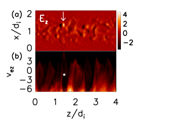
Figure 3: (a): Spatial structure of $E_{z}$ at $\Omega_{i}t=3$ in the current layer. (b): The phase space $z-v_{ez}$ at $x\sim 1.2$ of (a).

Magnetic reconnection induces a parallel electric field around the x-line and drives an intense electron beam. At $\Omega_{i}t=3$ ($\Omega_{i}=eB_{0}/m_{i}c$), the electron beams have been accelerated to $10c_{A}$ and to $14c_{A}$ at $\Omega_{i}t=4$. We show the current sheet around the x-line in the $x-y$ plane at $\Omega_{i}t=3.3$ in Fig. 1 (a). At the beginning of the magnetic reconnection simulation, the Buneman instability with wavevector along the magnetic field $z$ direction is excited. In the cold plasma limit, the phase speed is $(m_{e}/(2m_{i}))^{1/3}|v_{dz}|/2\sim 1c_{A}$ and the growth rate is $\gamma\sim\sqrt{3}\omega_{pe}(m_{e}/(2m_{i}))^{1/3}/2\sim 29\Omega_{i}$ (Galeev and Sagdeev, 1984). The Buneman instability saturates within a short time. Later in time two distinct spatial structures of the electric field are observed: localized bipolar structures dominate $E_{z}$ and long oblique stripes dominate $E_{x}$. A surprise is that there are two types of bipolar structures. At $\Omega_{i}t=3$ one has a velocity close to zero and the other moves with a velocity of $3c_{A}$. By $\Omega_{i}t=4$ the velocity of the second increases to $7c_{A}$. In Fig. 1 (b, c) we show $E_{z}$ and $E_{x}$ in the midplane $x-z$ of the current sheet at $\Omega_{i}t=3.3$. The structures move to the left in this figure, which is in the direction of the electron drift. The downward (upward) arrows point to fast (slow) moving electron holes. To see the two classes of holes more clearly, in Fig. 2 (a, b) we stack cuts of $E_{x}(z)$ and $E_{z}(z)$ at the x-line versus time. The dark and light bands mark the development of the bipolar structures seen in Fig. 1 (b, c). The slopes of these bands are the phase speeds of the waves. During the time interval $\Omega_{i}t=0-2$, the phase speed of the waves increases, which was expected since the streaming velocity of the electrons increased as the reconnection driven current layer shown in Fig. 1 (a) developed. During the time interval $\Omega_{i}t=2-4$ two distinct phase speeds, particularly in $E_{z}$, are evident. In Fig. 2 (b) the structures cross each other at the same value of $z$, which indicates that this result is not due to the spatial structure of the streaming velocity. In Fig. 3 we show $E_{z}$ and the $z-v_{z}$ phase space around $(x,y)=(1.2d_{i},1.5d_{i})$ at $\Omega_{i}t=3$ to reveal the structure of the fast moving holes. There are no slow holes in this region at this time. In (a) the most intense hole is marked by the arrow. In (b) the center of the $z-v_{ez}$ phase space of this bipolar structure is marked by the star. The electrons encircling the star indicate that electrons are trapped by the bipolar field. The strong electron heating due trapping is evident.

Electron holes in the simulation exhibit a complex dynmics: formation, dissipation and reformation. The lifetimes $\tau_{l}$ of the two classes of electron holes are distinct, around $0.1\Omega_{i}^{-1}$ and $0.2\Omega_{i}^{-1}$ for the fast and slow holes, respectively. In both $\tau_{l}$ exceeds the bounce time of the trapped electrons, $\tau_{b}\approx\sqrt{m_{e}\lambda_{b}}/\sqrt{2e\delta E_{z}}\sim 0.02\Omega^{-1}_{i}$, where $\lambda_{b}$ is the characteristic wavelength of the electron hole. Thus, electron trapping takes place and we therefore interpret the holes as BGK structures. (Bernstein et al., 1957).

3 Kinetic Model and Analytic Results

We now investigate which instabilities drive the two distinct types of holes by examining in more detail the development of streaming instabilities. Using two drifting Maxwellians to model the electron distribution and a single Maxwellian to model the ion distribution, we fit the distribution functions obtained from the simulations and substitute the theoretical fittings into the local dispersion function derived from kinetic theory for waves with $\Omega_{i}\ll\omega\ll\Omega_{e}$ (Che, 2009):

$$1+\frac{2\omega_{pi}^{2}}{k^{2}v^{2}_{ti}}[1+\zeta_{i}Z(\zeta_{i})]+\frac{2(1-\delta)\omega^{2}_{pe}}{k^{2}v^{2}_{te1}}[1+I_{0}(\lambda)e^{-\lambda}\zeta_{e1}Z(\zeta_{e1})]$$ (1)

$$+\frac{2\delta\omega^{2}_{pe}}{k^{2}v^{2}_{te2}}[1+I_{0}(\lambda)e^{-\lambda}\zeta_{e2}Z(\zeta_{e2})]=0,$$

where $\zeta_{i}=(\omega-k_{z}v_{di})/kv_{ti}$, $\zeta_{e1}=(\omega-k_{z}v_{de1})/k_{z}v_{zte1}$, $\zeta_{e2}=(\omega-k_{z}v_{de2})/k_{z}v_{zte2}$, $\lambda=k^{2}_{x}v^{2}_{xte}/2\Omega^{2}_{e}$, $\delta$ is the weight of the low velocity drifting Maxwellian, $Z$ is the plasma dispersion function and $I_{0}$ is the modified Bessel function of the first kind with order zero. The thermal velocity of species $j$ is defined by $v^{2}_{tj}=2T_{tj}/m_{j}$ and drift speed by $v_{dj}$, which is parallel to the magnetic field ($z$ direction). The electron temperature takes a different value along and across the magnetic field while the ions are taken to be isotropic.

The fitting parameters of the distribution functions at $\Omega_{i}t=3,4$ are listed in Table 1. The match between the parallel distribution and our fitted distribution is shown in Fig. 4 (a). We can see from the Table that the weight $\delta$ of the low velocity electrons increases with time, indicating that momentum is transferred from the high velocity to the low velocity electrons.

The theoretical 2D spectrum at $\Omega_{i}t=3$ is shown in Fig. 4 (b). Two distinct modes are found, one with $\mathbf{k}$ parallel and the other with $\mathbf{k}$ nearly perpendicular to $\mathbf{B}$. The peak of the parallel mode is around $k_{z}d_{i}\sim 20$, which is close to the wavenumber of the cold plasma limit of the Buneman instability, $k_{z}d_{i}=\omega_{pe}/v_{de}\sim 20$. To confirm that the parallel mode is the Buneman instability rather than the two-stream instability, we exclude ions from our calculations. The mode obtained only with electrons is shown in Fig. 4 (c). The two-stream instability has a much smaller growth rate. Thus, the parallel mode is the Buneman instability. The peak of the nearly-perpendicular mode is centered at $(k_{x}d_{i},k_{z}d_{i})=(22,5)$. The frequency of this mode is $\sim 13\Omega_{i}$ which is in the LH frequency range for the present simulation so the nearly-perpendicular mode is the LHI (McMillan and Cairns, 2006; Che et al., 2009).

As a test of this interpretation, we compare the phase speed of the modeled waves across ($v_{px}$) and along ($v_{pz}$) $\mathbf{B}$ with the simulation data. The assumption here is that since the fraction of trapped electrons in any given electron hole is small, the non-trapped particles control the phase speeds of the wave and the linear dispersion characteristics can be used to interpret hole propagation. It is well known that the Buneman instability can form parallel bipolar structures. This instability, which has a very low parallel phase speed to enable coupling to the ions, is the source of the electron holes moving slowly parallel to the magnetic field. Thus, the LHI should be responsible for the oblique, fast-moving electron holes marked by the downward arrows in $E_{z}$ and the oblique stripes in $E_{x}$ in Fig. 1. This interpretation is consistent with the parallel phase speeds $v_{pz}$ of the Buneman and LH instabilities obtained by the kinetic model which are shown in Fig. 2 (c). The phase speed of the Buneman instability with $\theta\sim 0$ is close to zero. The three arrows from left to right (black,red and green) indicate the position $\theta$ of the maximum-growing mode of the LH instability at $\Omega_{i}t=1,3,4$ shown in Fig. 2. The phase speed of the LH instability is initially low and then increases to $4c_{A}$ at $\Omega_{i}t=3$ and to $7c_{A}$ at $\Omega_{i}t=4$ . The high phase speed of the LHI is consistent with the fast-moving electron holes seen at late time in the simulation. As a further check on this interpretation, in Fig. 5 (a) we stack the cuts of $E_{x}(x)$ along $x$ at different times. The slope of the curves is the phase speed $v_{px}$. We see that at $\Omega_{i}t=3$ $v_{px}\sim 0.6c_{A}$. In (b) is the theoretical phase speed $v_{px}$ at $\Omega_{i}t=1,3,4$ calculated from the model. At $\Omega_{i}t=3$ the $v_{px}$ of the LH wave, marked with the “*”, is around $0.6c_{A}$, consistent with the value from the simulation.

4 Conclusion

In summary, we have demonstrated through simulations and an analytic model that two distinct classes of electron holes are generated simultaneously in the intense current layers that form during magnetic reconnection. The sources of the holes are the Buneman and LHI. The LH waves produce a transverse field $E_{x}$ as well as the bipolar structures $E_{z}$ that trap electrons to form electron holes. These electron holes move along the magnetic field at the phase speed of the LH wave. Electron holes formed by the Buneman instability move more slowly. The simultaneous existence of electron holes with two distinct phase speeds enables electron scattering over a much larger range of velocity space than would be possible by either either instability alone. Electron dissipation in the intense current layers that form during reconnection is therefore enhanced. The LH electron hole was also independently observed by 2D Vlasov simulations (Newman and Goldman, 2008).

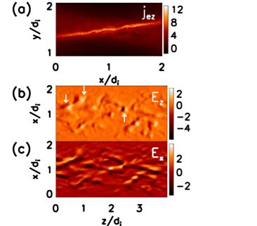
Figure 1: (a): The current sheet $j_{ez}$ in the $x-y$ plane at $\Omega_{i}t=3.3$. (b, c): The spatial structures of the electric fields $E_{x}$ and $E_{z}$ in the $x-z$ plane in a cut through the current layer.

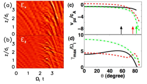
Figure 2: (a, b): Cuts of $E_{x}(z)$ and $E_{z}(z)$ around the x-line at different times from the simulation. (c): The theoretical parallel phase speed $v_{pz}$ vs. the angle $\theta$ between wavevector $\mathbf{k}$ and magnetic field at $\Omega_{i}t=1,3,4$ (black solid, red dashed and green dash-dotted lines). The arrows denote the angle $\theta$ of the fastest-growing mode of the LH instability at the three times in (d). (d) The theoretical growth rate $\gamma_{max}$ of fast-growing mode vs. the angle $\theta$ at the three times in (c).

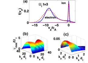
Figure 4: (a): Electron and ion distribution functions $f(v_{z})$ around the x-line at $\Omega_{i}t=3$ from simulations (blue solid) and the model (red-dashed) with the ion distribution function reduced by a factor of four. In (b) the 2D spectrum includes both electrons and ions and in (c) is without the ions.

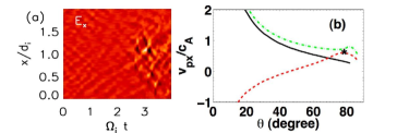
Figure 5: (a): Cuts of $E_{x}(x)$ at different times from the simulation. (b): Theoretical phase speed $v_{px}$ vs. $\theta$ at $\Omega_{i}t=1,3,4$, denoted by black solid, red-dashed and green dash-dotted lines.

Table 1: Parameters of Model Dist. Funs.

	$v_{xte}$	$v_{zte1}$	$v_{zte2}$	$v_{de1}$	$v_{de2}$	$v_{ti}$	$v_{di}$	$\delta$
$\Omega_{i}t$= 3	2.8	3.6	3.5	-9.0	-2.0	0.3	0	0.16
$\Omega_{i}t$= 4	2.8	4.0	4.2	-9.0	-5.0	0.34	0.1	0.26

References

- Andersson et al. (2009) Andersson, L., et al. (2009), New Features of Electron Phase Space Holes Observed by the THEMIS Mission, Phys. Rev. Lett., 102(22), 225,004–+, 10.1103/PhysRevLett.102.225004.
- Bernstein et al. (1957) Bernstein, I. B., J. M. Greene, and M. D. Kruskal (1957), Exact Nonlinear Plasma Oscillations, Physical Review , 108, 546–550, 10.1103/PhysRev.108.546.
- Cattell et al. (2005) Cattell, C., et al. (2005), Cluster observations of electron holes in association with magnetotail reconnection and comparison to simulations, J. Geophys. Res., 110, 1211–+, 10.1029/2004JA010519.
- Che (2009) Che, H. (2009), Non-linear Development of Streaming Instabilities in Magnetic Reconnection with a Strong Guide Field, Ph.D. thesis, University of Maryland, College Park, United States – Maryland.
- Che et al. (2009) Che, H., J. F. Drake, M. Swisdak, and P. H. Yoon (2009), Nonlinear Development of Streaming Instabilities in Strongly Magnetized Plasma, Phys. Rev. Lett., 102(14), 145,004–+, 10.1103/PhysRevLett.102.145004.
- Drake et al. (2003) Drake, J. F., M. Swisdak, C. Cattell, M. A. Shay, B. N. Rogers, and A. Zeiler (2003), Formation of Electron Holes and Particle Energization During Magnetic Reconnection, Science, 299, 873–877, 10.1126/Science.1080333.
- Farrell et al. (2002) Farrell, W. M., M. D. Desch, M. L. Kaiser, and K. Goetz (2002), The dominance of electron plasma waves near a reconnection X-line region, Geophys. Res. Lett., 29(19), 190,000–1.
- Fox et al. (2008) Fox, W., M. Porkolab, J. Egedal, N. Katz, and A. Le (2008), Laboratory Observation of Electron Phase-Space Holes during Magnetic Reconnection, Phys. Rev. Lett., 101(25), 255,003–+, 10.1103/PhysRevLett.101.255003.
- Galeev and Sagdeev (1984) Galeev, A. A., and R. Z. Sagdeev (1984), Wave-particles interactions, in Basic Plasma Physics: Selected Chapters, Handbook of Plasma Physics, Volume I, edited by A. A. Galeev and R. N. Sudan, pp. 683–711.
- Matsumoto et al. (2003) Matsumoto, H., X. H. Deng, H. Kojima, and R. R. Anderson (2003), Observation of Electrostatic Solitary Waves associated with reconnection on the dayside magnetopause boundary, Geophys. Res. Lett., 30(6), 060,000–1.
- McMillan and Cairns (2006) McMillan, B. F., and I. H. Cairns (2006), Lower hybrid turbulence driven by parallel currents and associated electron energization, Phys. Plasma, 13(5), 052,104–+, 10.1063/1.2198212.
- Newman and Goldman (2008) Newman, D. L., and M. V. Goldman (2008), Perpendicular Localization of Electron Holes by Spatially Inhomogeneous Flows During Magnetic Reconnection*, AGU Fall Meeting Abstracts, pp. B1735+.