A performance analysis of multi-hop ad hoc networks with adaptive antenna array systems

Abstract

Based on a stochastic geometry framework, we establish an analysis of the multi-hop spatial reuse aloha protocol (MSR-Aloha) in ad hoc networks. We compare MSR-Aloha to a simple routing strategy, where a node selects the next relay of the treated packet as to be its nearest receiver with a forward progress toward the final destination (NFP). In addition, performance gains achieved by employing adaptive antenna array systems are quantified in this paper. We derive a tight upper bound on the spatial density of progress of MSR-Aloha. Our analytical results demonstrate that the spatial density of progress scales as the square root of the density of users, and the optimal contention density (that maximizes the spatial density of progress) is independent of the density of users. These two facts are consistent with the observations of Baccelli et al., established through an analytical lower bound and through simulations in [1] and [2].

I Introduction

An ad hoc network is a collection of autonomous nodes that communicate in a decentralized fashion without relying on a pre-established infrastructure or on a control unit. The design of communication protocols and the analysis of their performance limits in this class of networks have been the subject of intense investigation over the last decade. This design involves the definition of strategies and procedures necessary for transferring data between the nodes of the network, namely, the development of medium access rules and routing algorithms. The analysis of the reliability of these protocols in the context of ad hoc networks is more complex than in the context of cellular or controlled networks because of the distributed nature of the former. New lines of research have been introduced using analytical tools from the theory of stochastic geometry. Stochastic geometry represents the nodes of the network as elements of a point process and studies their average behaviour under predefined communication strategies [3, 4]. This paper follows this methodology and proposes an analytical evaluation of the performance of two communication protocols under a random access strategy, namely, the multi-hop spatial reuse Aloha protocol (MSR-Aloha) [2], and the nearest receiver with forward progress (NFP) routing [5, 6]. In addition, this paper considers the quantification of the performance improvement that could be reached by employing adaptive antenna array systems. In point-to-point communication, multiple antennas can increase the link capacity by providing some form of diversity. In the presence of concurrent transmissions, the signals from multiple antennas can be combined to mitigate interference, and consequently, the link reliability is improved [7, 8]. The performance of multi-antenna systems in the context of ad hoc networks has been previously studied in [9, 10, 11, 12] (and references therein). However, unlike the work presented in the current paper, these previous works only consider single-hop communication. The main contribution of this paper is the derivation of a closed-form expression for the expected progress of packets (i.e., the mean distance covered in one hop by a transmitted packet toward its destination) under MSR-Aloha and NFP schemes, and with nodes employing adaptive antenna array systems. The mean progress allows to compute the spatial density of progress of the network, i.e., the mean distance traversed by all emitted packets per unit area toward their intended destinations in a single time slot, which in turn provides direct insight into the network transport capacity [1, 13]. The rest of this paper is organized as follows. Section II describes the system model and the communication protocols considered. In section III, we briefly discuss some related works and position the contribution of this paper. Sections IV and V present our analytical results as well as some numerical examples. Finally, section VI concludes the paper.

II System model

II-A Network model

We adopt the so-called stochastic geometric representation of ad hoc networks, which is described as a planar network formed by a set of nodes that are randomly located on the points of a homogeneous Poisson point process (PPP) with density $\lambda$ nodes per unit area. We assume that each node has an infinite number of packets to transmit, and access the common medium according to the slotted Aloha protocol, with a predefined transmission probability $p$. Thus, by the property of independent thinning of PPPs [3], the sets of transmitters and receivers form two independent homogeneous PPPs with density $\lambda^{t}=\lambda p$ and $\lambda^{r}=\lambda(1-p)$, respectively.

II-B Channel and capture models

We assume that every node uses a single transmit antenna and $L$ receive antennas. A transmitted signal undergoes both large-scale fading with a path-loss exponent greater than $2$, and small-scale Rayleigh fading. We assume that the channel coefficients do not vary during the transmission of one packet. A data packet is said to be successfully captured by a receiver node if the signal-to-interference-plus-noise ratio (SINR) perceived by this node exceeds a prefixed threshold $\beta$.
Formally, let us denote by $\Phi_{t}=\{X_{i},i\in\mathbb{N}\}$ and $\Phi_{r}=\{Y_{i},i\in\mathbb{N}\}$ the PPPs corresponding to the transmitter and the receiver sets, respectively; where the variables $X_{i}$ and $Y_{i}$ are random locations of transmitters and receivers, respectively. Consider an emitting node located at $X_{j}$ and a receiver node located at $Y_{k}$. The signal emitted by $X_{j}$ arrives at $Y_{k}$ corrupted by interference and noise. Thus the received signal vector is expressed as:

$$\mathbf{x}=|X_{j}-Y_{k}|^{-\alpha/2}\mathbf{h}_{jk}s_{j}+\sum_{X_{i}\in\Phi^{t}\setminus\{X_{j}\}}|X_{i}-Y_{k}|^{-\alpha/2}\mathbf{h}_{ik}s_{i}+\mathbf{n},$$ (1)

where $s_{i}$ is the signal emitted by node $X_{i}$; $\mathbf{h}_{ik}$ is the channel propagation vector between nodes $X_{i}$ and $Y_{k}$, that is distributed according to the multivariate complex Normal law with dimension $L$; $\mathbf{n}$ is a complex Gaussian noise vector, with variance $\sigma^{2}$ per dimension; $|X_{i}-Y_{k}|$ is the distance between $X_{i}$ and $Y_{k}$; and $\alpha$ is the path-loss exponent. In statistical antenna array processing, a weight vector is applied to the received signal, which is chosen based on the statistics of the data received and optimized under a given criterion. When the optimum vector, in the sense of SINR maximization, is applied, the resulting SINR is [7, 8]:

$$SINR_{jk}=|X_{j}-Y_{k}|^{-\alpha}\mathbf{h}_{jk}^{T}\mathbf{R}^{-1}\mathbf{h}_{jk},$$ (2)

where $\mathbf{R}$ is the interference-plus-noise covariance matrix expressed as: $\mathbf{R}=\sum_{X_{i}\in\Phi^{t}\setminus\{X_{j}\}}|X_{i}-Y_{k}|^{-\alpha}\mathbf{h}_{ik}\mathbf{h}_{ik}^{T}+\sigma^{2}\mathbf{I}_{L}$, the operator ^T denotes the Hermitian operator, and $\mathbf{I}_{L}$ is the identity matrix with dimension $L\times L$. In our paper [12], we have established the following key result on the probability of successful reception:

Proposition 1 ([12]):

Let $X_{i}$ and $Y_{j}$ be a transmitter and a receiver node. Employing the optimum combining detector, the probability of successful communication in a Poisson field of interferers and Rayleigh fading channel is:

$$\begin{array}[]{lcr}P_{s}(\lambda^{t},d_{ij},\beta,L)=&P(SINR_{ij}\geq\beta)&~{}\text{~{}~{}~{}~{}~{}~{}~{} ~{}~{}~{}~{}~{}~{}~{}~{}~{}~{}~{}~{}~{}~{}~{}~{}~{}~{}~{}~{} ~{}}\end{array}$$

$$\text{~{}~{}~{}~{}~{}~{}~{}~{}~{}~{}~{}~{}}=\sum_{k=0}^{L-1}\frac{(\lambda^{t}\Delta\beta^{2/\alpha}d_{ij}^{2}+\sigma^{2}\beta)^{k}}{k!}\exp{(-\lambda^{t}\Delta\beta^{2/\alpha}d_{ij}^{2}-\sigma^{2}\beta)},$$ (3)

where $d_{ij}=|X_{i}-Y_{j}|$, $\Delta=2\pi/\alpha\Gamma(2/\alpha)\Gamma(1-2/\alpha)$, and $\Gamma$ denotes the gamma function.

In order to simplify the mathematical analysis, the noise term will be ignored in the next sections. This simplification is reasonable since ad-hoc networks are interference-limited.

II-C Communication protocol

We will now describe the two communication schemes considered. A source node has a packet that it wishes to deliver to a distant destination. Unlike traditional routing protocols, no specific route (in terms of relays list) is determined in advance. At each time slot, a source (or a relay) node authorized to transmit selects the next relay, among the set of nodes in place, according to some predefined rules. In NFP routing, a transmitter selects the next relay to be its closest non-emitting node that lies in the direction of the final destination of the packet processed. Selecting the closest receiver allows the probability of successful communication to be maximized. However, this scheme implies short paths, which means a small spatial reuse factor. In the MSR-Aloha scheme, the next relay is selected to be the closest node to the final destination, among the set of receivers that successfully captured the data packet. This scheme provides the maximum possible progress toward the destination in each time slot, but needs the implementation of an elaborate relay selection procedure.

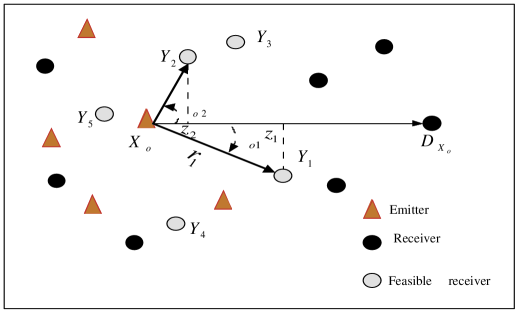
Figure 1: Simulation Results

Figure 1 shows an example of a snapshot of the network at an arbitrary time slot. The node $X_{o}$ is authorized to transmit, and has a packet for $D_{X_{o}}$. According to the NFP scheme, $Y_{2}$ is designated to be the next relay, since it is the closest receiver to $X_{o}$ in the direction of $D_{X_{o}}$. Because, in the case presented by figure 1, $Y_{2}$ can successfully capture the signal from $X_{o}$, the progress toward $D_{X_{o}}$, i.e., the distance travelled by the packet toward $D_{X_{o}}$, is equal to $|X_{o}D_{X_{o}}-Y_{2}D_{X_{o}}|$. This last quantity could be approximated by $z_{2}=r_{2}cos(\theta_{o2})$ if $|X_{o}D_{X_{o}}|\gg 1$. Among the set of non-emitting nodes, only $Y_{1},Y_{2},Y_{3},Y_{4}$, and $Y_{5}$ can successfully receive the packet. Applying the MSR-Aloha scheme, $Y_{1}$ is the next relay, since it is the closest to the destination, and thus provides the best progress.

III Related works

The idea of designing routing protocols with the notion of progress is first introduced in [5], where the authors propose the most forward within radius (MFR) routing. In MFR routing, an emitter selects its next relay, among the nodes within some given range from it, to be the nearest receiver to the destination. Baccelli et al. [1] propose the more sophisticated selection rule of the MSR-Aloha scheme described above. However, in their analytical framework, they find this selection rule to be difficult to manipulate, and so they apply some modifications to it. These modifications will be discussed and compared to our framework in the next sections. In [14], the authors propose and analyze the longest edge routing (LER), which applies a similar selection rule as MSR-Aloha. MSR-Aloha and LER differ in one key aspect that is that LER does not consider the direction of the intended destination, which is a challenging analytical aspect. It should be noted that all works cited do not consider the use of adaptive antenna array systems, which is one of the new aspects proposed in this work. Finally, practical implementation issues and complete simulation packages of MSR-Aloha routing are considered and detailed in [1, 2].

IV Performance analysis of NFP and MSR-Aloha schemes

IV-A Problem formulation

Before going through mathematical analyses, we must formally define some notions described in the previous section. Let $X_{i}\in\Phi_{t}$ be an arbitrary emitting node.

Definition 1 (Random set of feasible receivers):

The random set of feasible receivers for $X_{i}\in\Phi_{t}$ is formed by the subset of node in $\Phi_{r}\cup\{X_{i}\}$ that can capture the packet of $X_{i}$. Denoting this subset by $\mathcal{D}_{i}$, we have [1]:

$$\mathcal{D}_{i}=\left\{Y_{j}\in\Phi_{r}:SINR_{ij}\geq\beta\right\}\cup\{X_{i}\}$$ (4)

Definition 2 (Relay selection rules for NFP and MSR-Aloha):

Denoting by $Y^{*}_{NFP}$ and $Y^{*}_{MSR}$ the next relays selected by $X_{i}$ according to the NFP and MSR-Aloha schemes, respectively, we have:

$$Y^{*}_{NFP}=\arg\min_{Y_{k}\in\Phi_{r}:|\theta_{ik}|\leq\pi/2}|Y_{k}-X_{i}|,$$ (5)

and

$$Y^{*}_{MSR}=\arg\max_{Y_{k}\in\mathcal{D}_{i}}cos(\theta_{ik})|Y_{k}-X_{i}|,$$ (6)

where $\theta_{ik}$ is the angle between the two segments emerging from $X_{i}$ and pointing to the direction of its intended destination and to the direction of $Y_{k}$, respectively (Figure 1).

Note that, in definition 2, the quantity $cos(\theta_{ik})|Y_{k}-X_{i}|$ is an approximation on the progress, which is very accurate when the final destination is further away from the transmitter.

Definition 3 (Spatial density of progress):

The expected progress values for NFP and MSR-Aloha are computed as: $prog_{NFP}=\mathrm{E}\left[|Y^{*}_{NFP}|\cos\theta_{Y^{*}_{NFP}}P_{s}(\lambda^{t},|Y^{*}_{NFP}|,\beta)\right]$ and $prog_{MSR}=\mathrm{E}\left[|Y^{*}_{MSR}|\right]$, respectively. The spatial density of progress is simply equal to the transmission density times the expected progress.

IV-B Spatial average of progress derivation

IV-B1 NFP routing

Theorem 1:

The expected progress for NFP routing is:

$$prog_{NFP}(\lambda,p)=\frac{1}{\sqrt{\lambda}}\sum_{k=0}^{L-1}\frac{\Gamma(k+3/2)(\beta^{2/\alpha}\Delta)^{k}p^{k}(1-p)}{k!((1-p)\pi/2+\Delta\beta^{2/\alpha}p)^{k+3/2}}.$$ (7)

Proof.

The PPPs $\Phi_{r}$ and $\Phi_{t}$ are stationary (invariance by translation and rotation). Thus, we consider without any loss of generality, a typical emitter located at the center of the network ($X_{o}=(0,0)$) with an intended destination located on the horizontal axis. The distribution of the distance separating $X_{o}$ from its closest receiver in the direction of the destination verifies [3, 1]:

$$P(|Y^{*}_{NFP}|\leq r)=\exp{(-\frac{\lambda^{r}\pi}{2r^{2}})}.$$ (8)

Moreover, the angle between the direction of $Y^{*}_{NFP}$ and the horizontal axis is uniformly distributed in $[-\pi/2,\pi/2]$. Consequently, the average progress is:

$$\begin{array}[]{lcr}prog_{NFP}(\lambda,p)=&\mathrm{E}_{Y^{*}_{NFP}}\left[|Y^{*}_{NFP}|\cos\theta_{Y^{*}_{NFP}}P_{s}(\lambda^{t},|Y^{*}_{NFP}|,\beta)\right]&~{}\text{~{}~{}~{}~{}~{}~{}~{} ~{}~{}~{}~{}~{}~{}~{}~{}~{}~{}~{}~{}~{}~{}~{}~{}~{}~{}~{}~{} ~{}}\end{array}$$

$$\text{~{}~{}~{}~{}}=\int_{-\frac{\pi}{2}}^{\frac{\pi}{2}}\int_{0}^{\infty}r\cos\theta P(\theta)P(|Y^{*}_{NFP}|=r)P_{s}(\lambda^{t},r,\beta)drd\theta.$$ (9)

where $\mathrm{E}_{x}[\cdot]$ denotes the expectation with respect to the random variable $x$. Replacing $P_{s}(\lambda^{t},r,\beta)$ by its expression given by relation (9), we get the result of theorem 1. ∎

IV-B2 MSR-Aloha routing

As mentioned in section III, the MSR-Aloha scheme was previously analyzed by Baccelli et al. in [1]. However, rather than evaluating the mean progress according to the rule (6), the authors considered an approximation on it, which consisted in replacing the event of successful reception, i.e., $Y_{k}\in\mathcal{D}_{o}$ by its probability of occurrence. In other words, the following modified rule is used:

$$\tilde{Y}^{*}_{MSR}=\arg\max_{Y_{k}\in\Phi^{r}}P_{S}(\lambda,d_{ok},\beta)r_{k}\cos\theta_{k}.$$ (10)

The following proposition is demonstrated in [1].

Proposition 2:

The mean progress obtained when using the modified selection rule (10), denoted as $\widetilde{prog}_{MSR}(\lambda,p)$, is a lower bound on the mean progress associated to the selection rule (6), and is expressed as:

$$\widetilde{prog}_{MSR}(\lambda,p)=\frac{1}{\beta^{1/\alpha}\sqrt{\lambda p2\Delta\exp{(1)}}}\tilde{H}(p,\beta),$$ (11)

where $\tilde{H}(p,\beta)=\int_{0}^{1}1-\exp{\left(-\frac{1-p}{p}\frac{G(z)}{2\beta^{2/\alpha}\Delta}\right)}dz$, and $G(z)=2\int_{t:\frac{\exp{(t)}}{\sqrt{2\exp{(1)}t}}\leq 1/z}\arccos{\left(\frac{z\exp{(t)}}{\sqrt{2\exp{(1)}t}}\right)}dt$.

The lower bound (11) is difficult to evaluate numerically. Moreover, it concerns the case of a receiver with a single antenna, and cannot be easily generalized to the case of multi-antenna systems. We propose a direct manipulation of the selection rule (6), and we establish the following theorem.

Theorem 2:

The mean progress of MSR-Aloha verifies:

$$prog_{MSR}(\lambda,p)\leq\frac{1}{\beta^{1/\alpha}\sqrt{\lambda p\Delta}}H(p,L,\beta).$$ (12)

The function $H(p,L,\beta)$ does not dependent on $\lambda$, and is expressed as:

$$H(p,L,\beta)=\int_{0}^{\infty}1-\exp{\left(-\frac{1-p}{p}\frac{F(z)}{\beta^{2/\alpha}\Delta}\right)}dz,$$ (13)

where $F(z)=\sum_{i=0}^{L-1}\sum_{k=0}^{i}\frac{\Gamma(1/2+k)\Gamma_{inc}(1/2+i-k,z^{2})}{2k!(i-k)!}$, and $\Gamma_{inc}(k,z)=\int_{z}^{\infty}t^{k-1}\exp{(-t)}dt$ is the incomplete gamma function.

Proof.

Consider again the typical emitter $X_{o}$ and its intended final destination placed at the horizontal axis. The event that the progress, denoted $Z$, is less than some value $z$ is equivalent to the event that all the nodes that capture the packet are situated in the half-plane $D_{z}=\{(x,y):x\leq z\}$ ($(x,y)$ denotes the Cartesian coordinates of a point in the plane). Then we have:

$$\mathbf{1}_{(Z<z)}=\prod_{Y_{j}\in\Phi_{r}}(1-\mathbf{1}_{(SINR_{oj}>\beta)}\mathbf{1}_{(Y_{j}\notin D_{z})}),$$ (14)

where $\mathbf{1}_{\psi}$ denotes the indicator function, which is equal to $1$ when the propriety $\psi$ holds, and to $0$ otherwise. From (14), we have:

$$P(Z<z)=\mathrm{E}_{\Phi_{r},\Phi_{t}}\left[\prod_{Y_{j}\in\Phi_{r}}(1-\mathbf{1}_{(SINR_{oj}>\beta)}\mathbf{1}_{(Y_{j}\notin D_{z})})\right].$$ (15)

The right hand side of (16) corresponds to the expression of a probability generating functional. The probability generating functional of a PPP $\Psi(f)=\mathrm{E}_{\Phi}[\prod_{X\in\Phi}f(x)]$ is equal to $\exp{(-\lambda\int(1-f(X))dX)}$ [15, 14]. Consequently, the progress distribution verifies:

$$P(Z<z)=\mathrm{E}_{\Phi_{t}}\left[\exp{\left(-\lambda^{r}\int_{\mathbb{R}^{2}}\mathbf{1}_{(SINR_{Y}>\beta)}\mathbf{1}_{(Y\notin D_{z})}\right)}dY\right].$$ (16)

Applying the Jensen’s inequality to the last relation, we get:

$$P(Z<z)\geq\exp{\left(-\lambda^{r}\int_{\mathbb{R}^{2}}P_{s}(\lambda^{t},|Y|^{2},\beta)\mathbf{1}_{(Y\notin D_{z})}dY\right)}.$$ (17)

The integral in the right hand side is denoted by $In_{L}$, and evaluated as follows:

$$In_{L}(z)=\sum_{i=0}^{L-1}\int_{z}^{\infty}\int_{-\infty}^{\infty}\frac{(\gamma(x^{2}+y^{2}))^{i}}{i!}\exp{(-\gamma(x^{2}+y^{2}))}dydx.$$ (18)

where $\gamma=\lambda^{t}\Delta\beta^{2/\alpha}$. Substituting $x$ and $y$ by $u=\gamma x^{2}$ and $v=\gamma y^{2}$, respectively, we get:

$$In_{L}(z) = \sum_{i=0}^{L-1}\sum_{k=0}^{i}\frac{1}{\gamma k!(i-k)!}\int_{\gamma z^{2}}^{\infty}\frac{1}{2}u^{(i-k)-1/2}\exp{(-u)}du\cdot$$ (19)

$$\int_{0}^{\infty}v^{k-1/2}\exp{(-v)}dv$$

$$= \sum_{i=0}^{L-1}\sum_{k=0}^{i}\frac{\Gamma(1/2+k)\Gamma_{inc}(1/2+i-k,\gamma z^{2})}{2\gamma k!(i-k)!}.$$ (20)

The mean progress yields to:

$$prog_{MSR}(\lambda,p)\leq\int_{0}^{\infty}1-\exp{\left(-\lambda^{r}In_{L}(z)\right)}dz.$$ (21)

Applying the substitution $w=\sqrt{\gamma}z$, we get the result of theorem 2. ∎

V Discussion and numerical results

Analytical results show that the expected progress depends on the density $\lambda$ only through the factor $1/\sqrt{\lambda}$. Thus, the spatial density of progress scales as $\sqrt{\lambda}$, and the optimal contention density, i.e, the value of $p$ that maximizes the spatial density of progress, is independent of $\lambda$. This result is consistent with the scaling law of Gupta and Kumar [13], and with the observations of Baccelli et al., made through simulations in [2]. In the next, we present numerical and simulation results for NFP and MSR-Aloha. In the simulations, the network area is set at $10^{6}m^{2}$ with a density of nodes $\lambda=10^{-3}$. The experimental mean progress is obtained over $1000$ independent realizations of the network and results are normalized to a density equal to $1$.

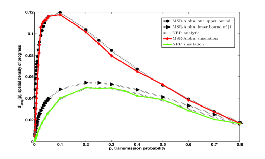
Figure 2: Simulation and analytical Results for MSR-Aloha and NFP routing, with $\alpha=4$, $\beta=1$, $\lambda=1$ and $L=1$.

Figure 2 presents the spatial density of progress as a function of the transmission probability, when the number of receive antennas is set at $1$. In the same figure, the lower bound on the MSR-Aloha spatial density of progress given by [1] is plotted. We observe that our analytical results are very accurate. The lower bound of [1] is indeed closer to the curve of NFP routing than to the curve of MSR-Aloha scheme, which is a result of the approximation considered in [1] that is explained as follows. The probability of capture decays exponentially with the distance, and consequently, the maximization of the product of the probability of success and the distance (selection rule (10)) is almost equivalent to taking the nearest receiver to the transmitter, i.e., the NFP scheme.

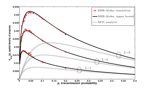
Figure 3: Spatial density of progress as a function of the transmission probability and the number of receive antennas, with $\alpha=3$, $\beta=10$, and $\lambda=1$. For some value of $p$ the experimental curves are above the upper bound. This fact is due to edge effects.

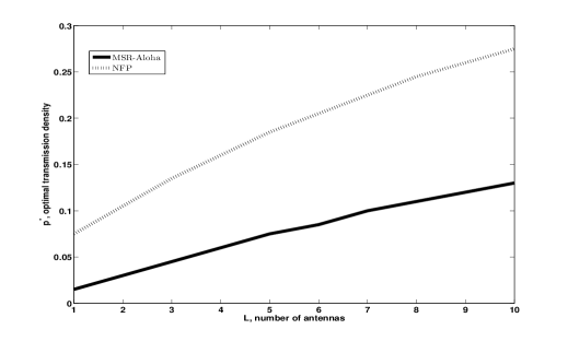
Figure 4: Optimal transmission density as a function of the number of receive antennas with $\alpha=3$, $\beta=10$, and $\lambda=1$.

Figure 3 shows that employing adaptive antenna array systems significantly improves the spatial density of progress. For example, with only one additional antenna, a $200\%$ gain is observed. This improvement is due to the additional diversity and interference cancellation capability provided by multi-antenna systems. Observe that the MSR-Aloha scheme is more sensitive to the transmission probability $p$ than is NFP routing, and this can be explained as follows: when $p$ increases, the interference becomes severe, leading to a decrease in the distance over which packets can be captured, and thus, to a significant decrease in $prog_{MSR}$. For the NFP scheme, the increase in $p$ produces both good and bad effects. In fact, a low value of $p$ means a high receiver density, and thus, a high number of receivers in the vicinity of each transmitter. Consequently, the selection of the nearest receiver results in a small amount of progress. On the other hand, increasing $p$ leads both to an increase in the distance separating each transmitter from its nearest receiver and to a reduction in the probability of successful reception, which explains the relatively slow variation of the NFP curve as compared to the MSR-Aloha curve.
Figure 4 presents the optimal contention probability as a function of the number of antennas. For the MSR-Aloha scheme, the optimal contention probability is equal to $0.015$ for single-antenna systems (with the parameters indicated on the figure, the same value was identified by means of simulations in [2]), and to $0.03$ and $0.045$ when using $2$ and $3$ antennas, respectively. Although NFP allows a higher optimal contention density, MSR-Aloha has a higher efficiency since it provides a better progress with a smaller number of transmission attempts.
Finally, several other simulations were done that show the influence of the parameters $\beta$ and $\alpha$, and these simulations are not presented here due to a lack of space.

VI Conclusion

This paper derived simple closed-form expressions for the mean density of progress of two communication strategies, namely MSR-Aloha and NFP routing. Our results quantify the improvement achieved through the use of adaptive antenna array systems. Analytical and simulation results show that MSR-Aloha protocol is highly efficient in terms of spatial density of progress and optimal contention probability. However, this scheme calls for implementation of a sophisticated relay selection procedure, which may introduce additional overhead. A fairer performance comparison of MSR-Aloha and other communication protocols must therefore take this aspect into consideration.

References

- [1] F. Baccelli, B. Blaszczyszyn, and P. Muhlethaler, “An aloha protocol for multihop mobile wireless networks,” IEEE Trans. Inf. Theory, vol. 52, no. 2, pp. 421–436, 2006.
- [2] ——, “Time-space opportunistic routing in wireless ad hoc networks: Algorithms and performance optimization by stochastic, geometry,” the Computer Journal, 2009, to appear.
- [3] D. Stoyan, W. Kendall, and J. Mecke, Stochastic Geometry and its Application, ser. Probability and Mathematical Statistics. Wiley, 1987.
- [4] M. Haenggi, J. G. Andrews, F. Baccelli, O. Dousse, and M. Franceschetti, “Stochastic geometry and random graphs for the analysis and design of wireless networks,” IEEE J. Sel. Areas Commun., vol. 27, no. 7, pp. 1029–1046, 2009.
- [5] H. Takagi and L. Kleinrock, “Optimal tarnsmission ranges for randomly distributed packet radio terminals,” IEEE Trans. Wireless Commun., vol. 22, no. 3, pp. 246–257, 1984.
- [6] S. Biswas and R. Morris, “ExOR: opportunistic multi-hop routing for wireless networks,” ACM SIGCOMM Computer Communication Review, vol. 35, no. 4, pp. 133–144, 2005.
- [7] C. A. Baird and C. Zham, “Performance criteria for narrowband array processing,” in IEEE Conference On Decision And Control, vol. 10, 1971, pp. 564–565.
- [8] H. Cox, R. M. Zeskind, and M. M. Owen, “Robust adaptive beamforming,” IEEE Trans. Acoust., Speech, Signal Process., vol. 35, pp. 1365–1375, 1987.
- [9] N. Jindal, S. P. Weber, and J. Andrews, “Rethinking MIMO for wireless networks: Linear throughput increases with multiple receiver antenna,” in IEEE ICC’09, 2009.
- [10] A. M. Hunter, J. Andrews, and S. Weber, “Transmission capacity of ad hoc networks with spatial diversity,” IEEE Trans. Wireless Commun., vol. 7, no. 12, pp. 5058–5071, 2008.
- [11] S. Govindasamy, D. W. Bliss, and D. H. Staelin, “Spectral efficiency in single-hop ad hoc wireless networks interference using adaptive antenna arrays,” IEEE J. Sel. Areas Commun., vol. 25, no. 7, pp. 1358–1369, 2007.
- [12] O. Ben-Sik-Ali, C. Cardinal, and F. Gagnon, “Performance of optimum combining in a poisson field of interferers and rayleigh fading channels,” IEEE Trans. Wireless Commun., submitted, minor revision, available at http://arxiv.org/abs/1001.1482.
- [13] P. Gupta and P. Kumar, “The capacity of wireless networks,” IEEE Trans. Inf. Theory, vol. 46, no. 2, pp. 388–404, 2000.
- [14] S. Weber, N. Jindal, R. Ganti, and M.Haenggi, “Longest edge routing on the spatial aloha graph,” in IEEE GLOBECOM’08, December 2008.
- [15] M. Westcott, “The probability generating functional,” Journal of the Australian Mathematical Society, vol. 14, pp. 448–466, 1972.