Intracluster stars in simulations with AGN feedback

Abstract

We use a set of high-resolution hydrodynamical simulations of clusters of galaxies to study the build-up of the intracluster light (ICL), an interesting and likely significant component of their total stellar mass. Our sample of groups and clusters includes AGN feedback and is of high enough resolution to accurately resolve galaxy populations down to the smallest galaxies that are expected to significantly contribute to the stellar mass budget. We describe and test four different methods to identify the ICL in cluster simulations, thereby allowing us to assess the reliability of the measurements. For all of the methods, we consistently find a very significant ICL stellar fraction ($\sim 45\%$) which exceeds the values typically inferred from observations. However, we show that this result is robust with respect to numerical resolution and integration accuracy, remarkably insensitive to changes in the star formation model, and almost independent of halo mass. It is also almost invariant when black hole growth is included, even though AGN feedback successfully prevents excessive overcooling in clusters and leads to a drastically improved agreement of the simulated cluster galaxy population with observations. In particular, the luminosities of central cluster galaxies and the ages of their stellar populations are much more realistic when including AGN. In the light of these findings, it appears challenging to construct a simulation model that simultaneously matches the cluster galaxy population and at the same time produces a low ICL component. We find that intracluster stars are preferentially stripped in a cluster’s densest region from massive galaxies that fall into the forming cluster at $z>1$. Surprisingly, some of the intracluster stars also form in the intracluster medium inside cold gas clouds that are stripped out of infalling galaxies.

1 Introduction

In optical observations, galaxy clusters appear as concentrations of galaxies on the sky. However, deep exposures reveal that not all the emission comes from stars that reside in the cluster’s member galaxies. Instead, there is also a smoothly distributed stellar component which is typically peaked around the cluster’s central galaxy, but extends to large radii. Due to its low surface brightness, observations of this intracluster light (ICL) component are difficult, resulting in a significant uncertainty in the current observational constraints of the amount of ICL present in clusters.

Lin and Mohr (2004) give an overview of the fractions of intracluster stars reported in the literature for different clusters and groups (see their Table 2). The reported values span a huge range from $\sim 2\%$ to $\sim 50\%$. Instead of analyzing very deep exposures of individual objects, Zibetti et al. (2005) stacked hundreds of cluster images from the Sloan Digital Sky Survey and masked all satellite galaxies, allowing them to obtain a very deep exposure of the brightest cluster galaxy (BCG) and the ICL of an average galaxy cluster. For a mean cluster mass of $7-8\times 10^{13}M_{\odot}$ they find that about $\sim 22\%$ of the stars reside in the BCG, while roughly $\sim 11\%$ are intracluster stars within a fixed aperture of 500 kpc. Gonzalez et al. (2005, 2007) describe another study for which a significant number of clusters and groups were observed. By analyzing the observed systems individually, they found that both the total stellar fractions as well as the relative fractions of stars residing in the BCG+ICL component strongly increase with decreasing halo mass. It was also concluded that intracluster stars are important for the baryon budget of clusters and groups.

The latter is particularly interesting in the light of the recent findings that the baryon fractions measured in clusters seem to be significantly lower than those inferred from the most current cosmological constraints (see e.g. McCarthy et al., 2007). However, no mechanism that can efficiently segregate baryons from dark matter on the scale of massive galaxy clusters is known. On the other hand, if there is indeed a significant component of intracluster stars, correctly accounting for them may relax the reported tensions.

The distribution and abundance of intracluster stars were also investigated based on cosmological hydrodynamical simulations of galaxy cluster formation that included radiative cooling and heating, as well as models for star formation and supernova feedback (Murante et al., 2004; Willman et al., 2004; Sommer-Larsen et al., 2005; Murante et al., 2007; Dolag et al., 2009). The origin of intracluster stars was studied in particular detail in Murante et al. (2007) finding an ICL fraction that rises with halo mass from $\sim 10\%$ at the group scale to $\sim 30\%$ for massive clusters. In their simulations, about half of the intracluster stars came from galaxies associated with the merger tree of the BCG, and most intracluster stars were liberated from their former host galaxies during merger events after redshift $z=1$. Using similar simulations but a different method to identify the ICL, Dolag et al. (2009) obtained average ICL fractions of around $\sim 33\%$, with a significant scatter on the group scale. No trend of the mean ICL fraction with halo mass was detected when their new ICL definition was used.

A major problem of most hydrodynamical cluster simulations thus far has been that they suffered from excessive “overcooling” within the densest cluster regions, where the gas cooling times are short. As a result, an unrealistically large fraction of cold gas and consequently a large amount of stars in clusters formed from the strong cooling flows. This in turn leads to central galaxies that are too bright and too blue, as well as extremely high total stellar fractions. It is widely believed that some source of non-gravitational energy input, like heating by active galactic nuclei (AGN), is necessary to offset the cooling in cluster cores and to make simulated clusters compatible with observations. In Sijacki et al. (2007) and Puchwein et al. (2008) it was shown that including a model for AGN feedback in such simulations, indeed, strongly improves the agreement between simulated and observed X-ray properties of clusters and groups (see also McCarthy et al., 2009).

In this work, we explore whether AGN feedback can also resolve discrepancies between simulated and observed cluster galaxy populations, and in particular, between the amount of intracluster light. Our high-resolution simulation set is well suited to investigate the origin of the ICL because for the first time a large simulated sample of galaxy clusters and group is available which can resolve the cluster galaxy populations down to very low galaxy masses and at the same time includes a successful model for the growth and feedback activity of AGN.

This paper is structured as follows. In Section 2 we describe our simulation set, the numerical models used, and the analysis methods we employ for measuring the ICL component in the simulations. We also summarize the tests we have carried out to investigate the robustness of our results with respect to numerical parameters and variations in the star formation model. In Section 3, we present our main results on the origin and amount of ICL found in our simulations, as well as on the properties of the simulated cluster galaxy populations. Finally, we summarize our findings and give our conclusions in Section 4.

2 Methods

We have carried out high-resolution cosmological hydrodynamical simulations of a large sample of galaxy clusters and groups, including a treatment of star formation and feedback processes. We will here mainly focus on analyzing the distribution of stars in the formed objects. To this end we develop and intercompare several distinct methods to measure the following components in our simulated clusters: the central galaxy (BCG), the satellite galaxies (i.e. all other cluster member galaxies), and the ICL. We then investigate the properties of these components and their relation to each other.

2.1 The simulations

Our simulated galaxy cluster and group sample is described in detail in Puchwein et al. (2008). In this work we use the 16 most massive objects of the sample. They approximately uniformly cover the mass range from $M^{\text{crit}}_{200}=2\!\times\!10^{13}M_{\odot}$ to $1.5\!\times\!10^{15}M_{\odot}$.

In brief, we have selected dark matter halos from the Millennium simulation (Springel et al., 2005b) at $z=0$ and resimulated them at higher mass and force resolution, including a gaseous component and accounting for hydrodynamics, radiative cooling, heating by a UV background, star formation and supernovae feedback. For each halo, at least two kinds of resimulations were performed. One containing the physics just described, and an additional one that also included a model for feedback from active galactic nuclei (AGN). We note that the original halo selection was only based on mass and otherwise random. New initial conditions for the resimulations were created by populating the Lagrangian region of each halo in the original initial conditions with more particles and adding additional small-scale power, as appropriate. At the same time, the resolution has been progressively reduced in regions that are sufficiently distant from the forming halo. Gas has been introduced into the high-resolution region by splitting each parent particle into a gas and a dark matter particle.

We have adopted the same flat $\Lambda$CDM cosmology as in the parent Millennium simulation, namely $\Omega_{\rm m}=0.25$, $\Omega_{\rm\Lambda}=0.75$, $h=0.73$, $n_{s}=1$ and $\sigma_{8}=0.9$. A baryon density of $\Omega_{\rm b}=0.04136$ has been chosen for consistency with the cosmic baryon fraction inferred from current cosmological constraints (Komatsu et al., 2008).

The simulations were run with the GADGET-3 code (based on Springel, 2005), which employs an entropy-conserving formulation of smoothed particle hydrodynamics (SPH). Radiative cooling and heating was calculated for an optically thin plasma of hydrogen and helium, and for a time-varying but spatially uniform UV background. Star formation and supernovae feedback were modelled with a subresolution multi-phase model for the interstellar medium as in Springel and Hernquist (2003a). Black hole growth and associated feedback processes were followed as in Springel et al. (2005a) and Sijacki et al. (2007).

Table 1 summarizes the different mass and force resolutions that were used in our resimulations. For all halos with $M^{\text{crit}}_{200}\leq 1.5\times 10^{14}\,h^{-1}M_{\odot}$ simulations with a zoom factor of 3 (see Table 1) have been performed, while all more massive cluster were resimulated only with a zoom factor of 2. For some objects several resimulations have been performed, covering a wide range in mass and force resolution. This allows us to assess the convergence of the simulations.

zoom	softening	particle mass $[h^{-1}M_{\odot}]$
factor	$[h^{-1}\textrm{kpc}]$	DM	gas	stars
1	7.5	$8.3\times 10^{8}$	$1.8\times 10^{8}$	$8.9\times 10^{7}$
2	3.75	$1.1\times 10^{8}$	$2.1\times 10^{7}$	$1.0\times 10^{7}$
3	2.5	$3.1\times 10^{7}$	$6.2\times 10^{6}$	$3.1\times 10^{6}$
4	1.875	$1.3\times 10^{7}$	$2.8\times 10^{6}$	$1.4\times 10^{6}$

Table 1: Force and mass resolutions used in the cluster and group simulations. The physical (Plummer-equivalent) softening lengths that were used for redshifts $z<5$ are listed in Column 2. For $z>5$, comoving softenings of $45\,h^{-1}{\rm kpc}$, $22.5\,h^{-1}{\rm kpc}$, $15\,h^{-1}{\rm kpc}$, and $11.25\,h^{-1}{\rm kpc}$ were used for zoom factors 1, 2, 3, and 4, respectively. The masses of the dark matter (DM), gas and star particles in the simulations are tabulated in Columns 3-5.

2.2 Identifying intracluster stars and cluster galaxies

Starting from the particle distribution in the simulated clusters, we aim to identify the cluster’s central galaxy, all satellite member galaxies and the ICL component. As a first step, we run a friends-of-friends (FoF) group finder with a linking length of 0.2 in units of the mean interparticle distance, as well as the SUBFIND substructure finder (Springel et al., 2001). The FoF algorithm is applied only to the high-resolution dark matter particles, with the gas and stars linked to their nearest dark matter particle. This avoids biases in the group catalogue due to the very different spatial distribution of dark matter and baryonic particles. We then use a version of SUBFIND that was specifically adapted to work robustly with hydrodynamical simulations (Dolag et al., 2008) for decomposing each FoF-group into a main halo and self-bound substructures. We consider the stellar content of each self-bound substructure of the cluster to be a satellite galaxy. All star particles that are part of the main halo are assumed to belong either to the BCG or to the ICL component. It is, however, not straightforward to unambiguously decide to which of these two components such a star particle should be assigned. In the following, we therefore employ several independent methods for making a distinction between the BCG and the ICL in simulated clusters. These are:

• Method 1: A cut-off radius around the central galaxy. The simplest possible approach is to just cut off the BCG at a specific radius $r_{\textrm{cut}}$. However, the size of BCGs correlates with cluster mass. We therefore choose to scale $r_{\textrm{cut}}$ with cluster mass. We obtain an appropriate scaling relation by combining an empirical relation between cluster mass and BCG luminosity (Popesso et al., 2007) with a relation between BCG luminosity and half-light radius $r_{\textrm{e}}$ (Bernardi et al., 2007). We decide to cut at $r_{\textrm{cut}}=3\times r_{\textrm{e}}$, yielding

  $$r_{\textrm{cut}}=27.3\,\,h^{-1}\textrm{kpc}\times\left(\frac{M^{\text{crit}}_{200}}{10^{15}\,h^{-1}M_{\odot}}\right)^{0.29}.$$ (1)

  When using this method, all star particles of the main halo that are within the cut-off radius are considered to be part of the BCG, while all main halo star particles outside this radius are considered to be intracluster stars.

• Method 2: Analysis of the surface brightness profiles. A de Vaucouleurs profile (de Vaucouleurs, 1948) is usually a good fit to the surface brightness profile of an elliptical galaxy. For cD galaxies, however, one often finds a light excess at large radii with respect to such a fit to the inner region (Schombert, 1986). This light excess can be attributed to intracluster stars.

  The complete surface brightness profile of BCG and ICL can typically be well fit by the sum of two de Vaucouleurs profiles (see e.g. Gonzalez et al., 2005). We perform such a two-component fit to the surface brightness profile of all stars residing in a simulated cluster’s main halo, as found by SUBFIND, and consider the component with the smaller effective radius as the BCG and the component with the larger effective radius as the ICL. This procedure is illustrated for a cluster with $M^{\text{crit}}_{200}=2.2\times 10^{14}\,h^{-1}M_{\odot}$ in Fig. 1. We note that we obtain projected mass profiles for the BCG and the intracluster stars by assuming that in each radial bin both components have the same mass-to-light ratio. In order to compute surface brightness profiles we use the stellar population synthesis model library GALAXEV (Bruzual and Charlot, 2003) to assign a r-band luminosity to each star particle according to its mass, age and metallicity.

• Method 3: Analysis of the stellar velocity distribution. In relaxed simulated clusters, the distribution of the velocities $v$ of the main halo stars can be well fit by a sum of two Maxwell-Boltzmann distributions (see Dolag et al., 2009). Here $v$ is given by $v=|{\mn@boldsymbol{v}}_{\textrm{star}}-{\mn@boldsymbol{v}}_{\textrm{clus}}|$, where ${\mn@boldsymbol{v}}_{\textrm{star}}$ is the velocity of the star particle and ${\mn@boldsymbol{v}}_{\textrm{clus}}$ is the velocity of the centre of mass of the cluster’s main halo. In this method, we perform such a fit for each cluster and define the BCG mass as the mass of the stars in the Maxwell-Boltzmann component with the lower velocity dispersion, while we associate the higher dispersion component with the ICL. This is illustrated in Fig. 2 for a cluster with mass $M^{\text{crit}}_{200}=2.2\times 10^{14}\,h^{-1}M_{\odot}$.

• Method 4: Analysis of the stellar velocity distribution and binding energies. While Method 3 allows an estimate of the total stellar BCG mass, it does not assign individual star particles to either the BCG or ICL component, as it yields, for each velocity bin, only the fraction of stars in each component. However, by also including the binding energies of the star particles in the analysis, the method can be extended to allow such an individual assignment, as discussed in full detail in Dolag et al. (2009).

  In short, we use this approach in the following way. We start with the two component Maxwell-Boltzmann fit obtained from Method 3. Then we use an iterative algorithm that assigns star particles according to their binding energy either to the BCG or to the ICL, with the iteration repeated until the BCG and ICL velocity distributions roughly match the fitted Maxwell-Boltzmann components. We start the iteration with some value $r_{\textrm{grav}}$ for the size of the BCG’s gravitating mass distribution. Then, the gravitational potential of all simulation particles with a distance $r<r_{\textrm{grav}}$ from the cluster centre is computed. All main halo star particles that are bound in this potential are assigned to the BCG in this iteration step, while unbound main halo stars are assigned to the ICL. Next, the velocity dispersion of the ICL component is calculated and compared to the velocity dispersion of the two Maxwell-Boltzmann fits. If the velocity dispersion of the ICL is too large, $r_{\textrm{grav}}$ is reduced to unbind more of the slowly moving particles. Otherwise, $r_{\textrm{grav}}$ is increased. We stop the iteration once the ICL velocity dispersion agrees with the velocity dispersion of the higher dispersion Maxwell-Boltzmann component to within 1%. Fig. 2 displays the resulting velocity distributions of the BCG and ICL components obtained in this way and compares them to the corresponding Maxwell-Boltzmann fits.

In Fig. 1, we compare the dynamical definition of BCG and ICL obtained with Method 4 to the analysis of the surface brightness profiles used in Method 2. For the shown cluster the agreement between these two completely different methods is remarkably good. However, in some other clusters the differences are admittedly larger (see also Fig. 6).

Figure 1: r-band surface brightness profiles of main halo stars of a $2.2\times 10^{14}\,h^{-1}M_{\odot}$ cluster. The red solid curves show the surface brightness profile of all main halo stars and its two-component de Vaucouleurs fit (smooth curve). The straight green dashed and blue dotted lines indicate the two individual de Vaucouleurs components corresponding to the BCG and ICL. The additional green dashed and blue dotted curves indicate the surface brightness profiles of the BCG and ICL as found by Method 4. For this cluster the results of Method 2 and Method 4 agree very well. The $r$-axis has been chosen to be linear in $r^{1/4}$. The simulation has been performed without AGN feedback.

Figure 2: Velocity distribution of main halo stars of a $2.2\times 10^{14}\,h^{-1}M_{\odot}$ cluster. The red solid histogram shows the velocity distribution of all main halo stars. The smooth red solid curve is the two component Maxwell-Boltzmann fit used in Method 3 and 4. The smooth green dashed and blue dotted curves indicate the individual Maxwell-Boltzmann distributions corresponding to the BCG and ICL. The green dashed and blue dotted histograms show the velocity distributions of the BCG and ICL as identified by Method 4. The simulation has been performed without AGN feedback.

We note that we can obtain a BCG and ICL mass by all of these four methods. However, only Method 1 and Method 4 allow us to individually assign each main halo star particle to one of these two components.

2.3 Robustness with respect to numerical resolution and integration accuracy

Before we apply the methods introduced above to our full cluster and group sample, we investigate whether our satellite galaxy, BCG and ICL stellar masses are robust with respect to numerical resolution by analysing three halos that were simulated at several different mass and force resolutions. We also test our integration accuracy with one further cluster simulation where we used two times smaller time steps and a higher force accuracy setting in our tree code.

Fig. 3 shows the masses of all stars, of all main halo stars (i.e. BCG+ICL), and of the BCG in these test simulations for a group with $M^{\text{crit}}_{200}=4.4\times 10^{13}\,h^{-1}M_{\odot}$ and a cluster with mass $M^{\text{crit}}_{200}=1.5\times 10^{14}\,h^{-1}M_{\odot}$. We computed these masses within $r^{\text{crit}}_{500}$, based on resimulations with zoom factors 1, 2, and 3, without inclusion of AGN physics. The BCG masses obtained with all the four different methods introduced in Sect. 2.2 are shown. The total stellar masses are well converged even in our lowest resolution simulations without AGN. However, the mass of stars in satellite galaxies, which is given by the difference between the results shown for all stars and for the BCG+ICL component, is not fully converged at the resolution of zoom factor 1. On the other hand, the results for zoom factors 2 and 3 for the BCG+ICL and the satellite galaxy mass agree very well, indicating that for zoom factor 2 and larger good convergence is achieved.

The BCG masses that are inferred with the different analysis methods can sometimes slightly differ from each other. This will be discussed in more detail in Section 3.1.2. Here, we want to assess the numerical convergence of the results obtained by each individual method. The BCG masses obtained by using a cutoff radius (Method 1) or the surface brightness profile analysis (Method 2) are already roughly converged even at the zoom factor 1 resolution. The results for Method 3 and Method 4 on the other hand, which both rely on fitting the velocity distribution of main halo stars, seem to be somewhat more easily affected by low numerical resolution, because the masses obtained for zoom factor 1 are larger than those obtained from the higher resolution runs. However, at least for the group shown in the left panel of Fig. 3, this seems partly due to a slightly different timing of a rather massive subhalo that is just passing by close to the cluster center in the low resolution simulation, so it is not really clear how generic this effect is. In any case, we find that the BCG masses have robustly converged at zoom factors 2 and larger.

Figure 3: BCG, BCG+ICL and total stellar mass found within $r^{\text{crit}}_{500}$ in a $4.4\times 10^{13}\,h^{-1}M_{\odot}$ group (left panel) and a $1.5\times 10^{14}\,h^{-1}M_{\odot}$ cluster (right panel) simulated without AGN at different numerical resolutions. Results are shown for zoom factor 1, 2, and 3 resolutions (see Table 1) as well as for the four different methods for determining a BCG mass (see Sect. 2.2). In the right panel, two zoom factor 2 simulations are shown, one with the standard parameters (a) and one with smaller time steps and a more accurate force computation (b). Results are well converged for zoom factors 2 and larger.

However, we also find that the resolution requirements to obtain converged results for the total stellar mass in runs with AGN feedback are somewhat higher. This is because at higher resolution star formation shifts to smaller halos, which contain smaller black holes that are less effective in suppressing star formation by their feedback. As a consequence, the total stellar mass in our simulated clusters is not nearly as well converged at the resolution of zoom factor 1 as in our runs without AGN. It is, however, reasonably converged at zoom factor 2 (stellar mass about $\sim 20\%$ low) and well converged at zoom factor 3 resolution (about $\sim 6\%$ low).

The results of the run with smaller time steps and higher force accuracy agree extremely well with those obtained form the corresponding run with our standard numerical parameters (see right panel of Fig. 3). We hence conclude that the orbit integration is sufficiently accurate in our simulations. This is important and reassuring, as an insufficient integration accuracy may lead to an artificially enhanced stripping rate of stars out of cluster galaxies.

In Fig. 4, we explore the convergence of the properties of the satellite galaxy population in more detail. Here the combined stellar mass of all satellite galaxies whose individual stellar masses exceed $M$ is shown as a function of $M$ for simulations at different resolution. Comparing the curves obtained from simulations with zoom factors 1, 2, 3, and 4, we conclude that the satellite galaxy population is reasonably converged for stellar masses larger than $\sim 5\times 10^{10}\,h^{-1}M_{\odot}$, $\sim 6\times 10^{9}\,h^{-1}M_{\odot}$ and $\sim 2\times 10^{9}\,h^{-1}M_{\odot}$, at zoom factors 1, 2 and 3, respectively. In other words, the formation, merger and tidal disruption rates of galaxies above these masses should be robust with respect to numerical resolution. Using the double Schechter fit to the observed galaxy stellar mass function from Baldry et al. (2008), we estimate that $\sim 69\%$, $\sim 17\%$ and $\sim 9\%$ of the total stellar mass are contained in galaxies with individual stellar masses below these resolution limits. Thus, at zoom factor 1 the majority of stars resides in poorly resolved galaxies. This explains why we obtain lower values for the mass in satellite galaxies in these runs (see Fig. 3). On the other hand, in the runs with zoom factors 2 and 3, the vast majority of stars resides in galaxies whose abundance is numerically converged. We thus do not expect a significant spurious contribution to the ICL component form underresolved galaxies in these simulations.

Figure 4: Combined stellar mass of all satellite galaxies with individual stellar masses exceeding $M$ as a function of galaxy stellar mass $M$. Results are shown for zoom factor 1, 2 and 3 simulations of a $M^{\text{crit}}_{200}=1.5\times 10^{14}\,h^{-1}M_{\odot}$ cluster and zoom factor 3 and 4 simulations of a $M^{\text{crit}}_{200}=3\times 10^{13}\,h^{-1}M_{\odot}$ group. No AGN have been included in these runs. The vertical lines, arrows and, labels (zf1), (zf2), and (zf3) indicate the galaxy mass ranges in which the stellar mass in satellite galaxies is approximately converged in zoom factor 1, 2, and 3 simulations, respectively.

Overall, these test simulations indicate that the distribution of stars in our cluster resimulations with zoom factors 2 and 3 are robust with respect to mass and force resolution, except for maybe a slight underestimation of the total star formation efficiency in zoom factor 2 runs that include AGN. Importantly, we have also verified that our results are invariant when the time step size is reduced or the accuracy of the gravitational force computation is improved.

2.4 Dependence on the star formation model

We also investigated how sensitive our results are to changes in the parameters of the star formation model. More precisely, we performed two test simulations, one with a higher gas density threshold for star formation, and another one in which we assumed a larger timescale for the conversion of gas into stars.

The idea behind using a higher gas density threshold was that this might lead to smaller and denser galaxies, which should then be less prone to tidal stripping. This in turn could reduce the amount of ICL in the simulated clusters. In one of our tests, we therefore increased the threshold density for star formation by a factor of $\sim 4$ compared to the original simulation. Within the subresolution model of Springel and Hernquist (2003a) for the regulation of star formation this was achieved by increasing the ‘supernova temperature’ $T_{\text{SN}}$ from $10^{8}\text{K}$ to $4\times 10^{8}\text{K}$, as well as the supernova evaporation factor $A_{0}$ from 1000 to 4000, while keeping the gas consumption timescale the same. However, the analysis of this simulation yielded very similar results to the original run. The fraction of stars in the BCG+ICL component changed by only about $1\%$.

Varying instead the timescale for star formation and thereby shifting the peak of the star formation activity to a different stage in the assembly history of the cluster might also affect the ICL component. In particular, since mergers play an important role in liberating stars from their host galaxies (see Murante et al., 2007), the efficiency of this mechanism for creating ICL stars may depend on the star formation history of the cluster. The idea behind our second test of the star formation model was therefore to increase the timescale $t_{0}^{*}$ for the conversion of gas into stars from 2.1 Gyrs to 8.4 Gyrs. Keeping everything else equal, this required again to set $T_{\text{SN}}=4\times 10^{8}\text{K}$ and $A_{0}=4000$ to leave the gas density threshold at its original value, while $t_{0}^{*}$ itself was increased by a factor of 4. Using this larger gas consumption timescale indeed shifts the peak of the star formation history to much later times and broadens it at the same time. It also results in more star formation at low redshift. However, also for this simulation we find remarkably little difference in the galaxy population and the ICL compared to the original run. Despite the substantial change in the star formation history, the fraction of stars in the BCG+ICL component increased by only $4\%$.

Overall, these tests show that the fraction of stars that get unbound from their host galaxies and become intracluster stars is remarkably insensitive to the detailed parameters of the star formation model.

3 Results

We now turn to the presentation of our primary results, obtained by applying the methods introduced in Sect. 2.2 to our full sample of simulated clusters. In particular, we investigate what fraction of a cluster’s stellar mass resides in the BCG, the ICL, and in the satellite galaxies. We also study whether the answer to this question depends on cluster mass. Finally, we examine where the stars that end up in these three components at redshift $z=0$ are formed, and in what objects they fall into the cluster.

3.1 Intracluster light, satellite galaxies, and BCGs in simulations and observations

3.1.1 The baryonic mass fractions

Figure 5 illustrates the baryon and stellar mass fractions of our simulated clusters, as well as the mass fraction of stars that reside in cluster galaxies as a function of cluster mass $M_{500}^{\textrm{crit}}$. Results from simulations both with and without AGN feedback are shown, and for comparison with observational constraints, data from Gonzalez et al. (2007), Giodini et al. (2009) and Lin et al. (2003) are included.

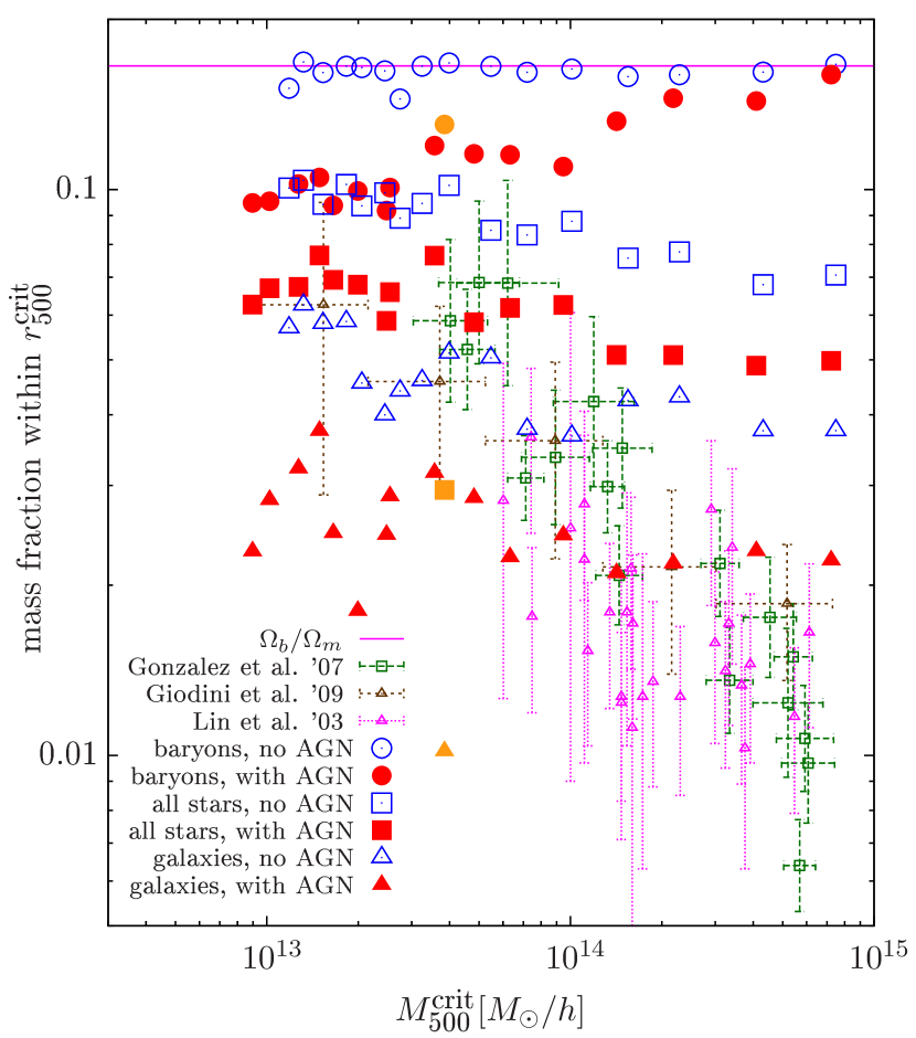
Figure 5: Mass fraction of baryons (circles), all stars (including ICL, squares), and stars residing in galaxies (triangles) within $r_{500}^{\textrm{crit}}$ for clusters and groups simulated with and without AGN feedback. The latter was found by summing up the stellar masses of the BCG, which was found by Method 1, and all satellite galaxies within $r_{500}^{\textrm{crit}}$. Observational data are shown for comparison. The Gonzalez et al. (2007) data should be compared to the mass fraction of all stars, while the other observational data should be compared to the mass fraction of stars found in galaxies. The cosmic baryon fraction assumed in the simulations is shown for reference. The orange symbols show results of a simulation where also kinetic supernova feedback was included.

In the simulations without AGN feedback, the baryon mass fractions within $r_{500}^{\textrm{crit}}$ differ by less than $\sim 10\%$ from the assumed cosmic baryon fraction. When AGN are included, this holds only for the most massive clusters, while there is a significant baryon depletion in poor clusters and groups due to the AGN heating (see also Puchwein et al., 2008).

Without AGN, we obtain very large stellar mass fractions. In massive clusters, roughly $40\%$ of the baryonic mass is found in stars, while on the group scale this number rises to about $60\%$. This seems to be inconsistent with observations, especially for massive clusters. When AGN are included, the stellar mass fractions within $r_{500}^{\textrm{crit}}$ are lowered by about one third. One can compare these total stellar mass fractions to the constraints from Gonzalez et al. (2007), as both cluster galaxies and intracluster stars were accounted for in that study. The simulated and observed stellar mass fractions are in good agreement on the group scale. However, we do not find a comparably strong trend with halo mass in our simulations as inferred by Gonzalez et al. (2007), and accordingly we obtain significantly larger stellar mass fractions for massive clusters.

Also shown in Fig. 5 is the mass fraction of stars in cluster galaxies. More precisely, these values were calculated by summing up the stellar masses of the BCG, which was found by Method 1, i.e. using the radial cut-off scaled with the cluster mass, and of all satellite galaxies within $r_{500}^{\textrm{crit}}$. The resulting values can be compared to the mass fractions of stars in cluster galaxies obtained by Giodini et al. (2009) and Lin et al. (2003). Without AGN, we again find a significant discrepancy for massive clusters. Compared to the observations the combined stellar mass of the cluster galaxies is too large. Also on the group scale the mass fractions in the simulations are larger than those from Lin et al. (2003). However, they are roughly consistent with the Giodini et al. (2009) results there. When AGN feedback is included the combined stellar mass of the cluster galaxies drops by about $\sim 40\%$. This substantially improves the agreement with observations for massive clusters. On the group scale, there is then good agreement with the Lin et al. (2003) data, while Giodini et al. (2009) inferred slightly larger mass fractions there.

Overall, the stellar mass fractions obtained without AGN feedback are clearly too large. When the effects of AGN heating are included, the stellar mass in cluster galaxies becomes however almost consistent with observations. In particular, the total stellar mass, i.e. including the ICL, agrees with the Gonzalez et al. (2007) results on the group scale. However, for massive clusters, we find a much larger ICL contribution in the simulations than they infer from observations. The simulations also do not fully reproduce the observed strong trend of the stellar mass fractions with halo mass.

One should mention that we did not include kinetic supernova feedback in the present set of simulations, instead all feedback from star formation was injected thermally. Using supernova feedback that includes a kinetic component can significantly reduce the amount of stars formed in hydrodynamical cosmological simulations (e.g Springel and Hernquist, 2003b; Borgani et al., 2006). While this might help to reproduce the overall stellar mass fractions in massive clusters, it is, considering that such simulations (see Borgani et al., 2006) also find only a weak trend of stellar mass fractions with halo mass, unlikely to significantly improve the overall agreement with observations. Nevertheless, we repeated the simulation of one of our clusters, this time including a strong kinetic supernova feedback component, in order to assess how it changes the fraction of stars found in the BCG, the ICL, and in the satellite galaxies. This run also included AGN feedback. Its results are indicated by orange symbols in Fig. 5. The corresponding simulation without winds, is the one indicated by the red symbols at almost the same (slightly lower) $M_{500}^{\textrm{crit}}$.

3.1.2 The stellar fractions in the BCG, ICL, and satellite galaxies

In the following, we discuss what fraction of stars in our simulated clusters and groups reside in the BCG, the ICL, and in the satellite galaxies, and how this compares to observations. Fig. 6 shows the mass fractions of the stars found in the BCG and in the whole main halo, i.e. in the BCG+ICL component. The values were calculated within $r_{500}^{\textrm{crit}}$. Results obtained from simulations both with and without AGN are shown. The BCG fractions are reported for all the four different methods we used to determine a BCG mass (see Sect. 2.2). For reference, observational constraints on the BCG+ICL luminosity fraction from Gonzalez et al. (2007) are also shown. They should be compared to the simulated BCG+ICL luminosity fractions indicated in the plot. The latter were computed within a projected radius (rather than a 3D radius) of $r_{500}^{\textrm{crit}}$, using the same method to obtain stellar luminosities as described in Sect. 2.2.

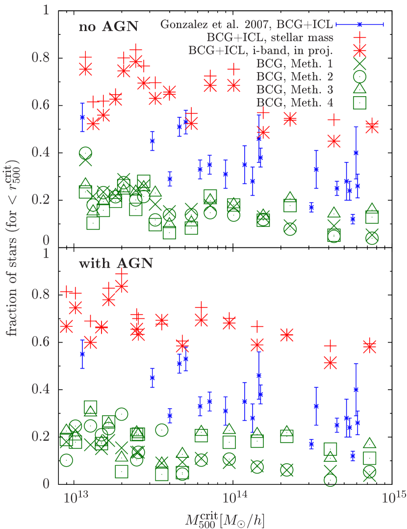
Figure 6: Fraction of the stellar mass within $r_{500}^{\textrm{crit}}$ found in the BCG, and in the BCG+ICL component. Mass fractions are shown as a function of cluster mass $M_{500}^{\textrm{crit}}$ and for the four different methods of determining a BCG mass (see Sect. 2.2). The upper panel shows the values computed from runs without AGN, while the lower panel illustrates the results obtained when including the AGN feedback. Also shown is the BCG+ICL i-band luminosity fraction within a projected radius on the sky (rather than 3D radius) of $r_{500}^{\textrm{crit}}$. This data can be directly compared to the observed BCG+ICL luminosity fractions from Gonzalez et al. (2007).

Without AGN, we obtain BCG+ICL fractions of roughly $\sim 50\%$ for massive clusters, and of about $\sim 70\%$ for groups. Note, however, that these values are sensitive to the radius inside which they are measured, because the distribution of the BCG+ICL component is more concentrated than the distribution of the satellite galaxies. For example, within $r_{200}^{\textrm{crit}}$ the values drop to about $\sim 45\%$ and $\sim 65\%$, respectively. Accordingly, the BCG+ICL fractions are also lower when calculated within a projected radius rather than a 3D radius equal to $r_{500}^{\textrm{crit}}$. However, the BCG+ICL luminosity fractions indicated in the figure are also affected by small differences in the mass-to-light ratio. Namely, we find mass-to-light ratios for the BCG+ICL components that are a few percent smaller (up to  10% smaller for massive cluster, while being almost identical for groups) than those of the whole stellar population in the simulated halo. Thus, the i-band luminosity fractions are only slightly smaller than the mass fractions calculated within a 3D radius equal to $r_{500}^{\textrm{crit}}$. When accounting for these effects, we nevertheless still obtain larger BCG+ICL fractions than derived from the observations of Gonzalez et al. (2007), especially for massive clusters.

When AGN feedback is included, the stellar mass of the BCG+ICL component decreases by about $\sim 25\%$. However, the total stellar masses decrease somewhat more strongly (see Fig. 5). Thus, we find even slightly larger BCG+ICL fractions in the simulations with AGN. A potential explanation for this effect is that galaxies falling into the cluster in simulations with AGN may be more prone to tidal disruption due to their lower stellar mass and due to an expansion of their halos as a consequence of the removal of gas by AGN heating.

Especially in the runs without AGN, there are several clusters for which all the four different analysis methods for identifying the BCG yield very similar BCG fractions and masses (see also Fig. 1). There are, on the other hand, also clusters where the results differ. In most of them, however, there is still good agreement between the two methods that were inspired by observational approaches, i.e. between Method 1, where a radial cut-off is used, and Method 2, where surface brightness profiles are analyzed. Also, the methods that rely on the dynamics, i.e. Method 3 and Method 4, usually agree well with each other, even though this is perhaps not too surprising as they both are based on the same fit of the stellar velocity distribution. In the rare cases were they do disagree, it is typically in unrelaxed objects, e.g. when an infalling group perturbs the stellar velocity distribution and prevents an accurate two-component Maxwell fit.

Overall, there is hence some uncertainty in the BCG mass due to the choice of the analysis method used for separating the BCG from the ICL. However, for all our different methods only a small part of the stars in the main halo, i.e. in the BCG+ICL component, may be assigned to the BCG. This also means that independent of how exactly we choose to make a distinction between BCG and ICL, we find a very significant ICL component in our simulated clusters and groups. We also note that the BCG and ICL components in Gonzalez et al. (2005) are defined very similarly to our Method 2, hence our analysis method should yield results that can be directly compared to observations.

The fraction of stars in the ICL can be read off form the difference between the BCG+ICL and BCG fractions in Fig. 6. As can be seen, the ICL fractions in our simulations are almost independent of the cluster mass. Within $r_{500}^{\textrm{crit}}$, they are roughly $\sim 45\%$ without AGN and $\sim 50\%$ with AGN physics. If we go to the larger radius of $r_{200}^{\textrm{crit}}$ instead, they are slightly lower, that is about $\sim 40\%$ without AGN and $\sim 45\%$ with AGN.

At a first glance these findings seem to be at odds with the results of Murante et al. (2007), where an ICL fraction rising with cluster mass was found, from $\sim 15\%$ at $10^{14}\,h^{-1}M_{\odot}$ to $\sim 30\%$ at $10^{15}\,h^{-1}M_{\odot}$. However, the lower values they obtained are most likely a consequence of the much lower numerical resolution in their simulations, as they explicitly exclude stars from the ICL that got liberated from poorly resolved galaxies. Looking only at the three clusters they have simulated at high resolution, i.e. with a mass resolution comparable to our simulations, there is no significant discrepancy. For those three objects they find ICL fractions of $37\%$, $28\%$, and $41\%$, and no strong indication of a dependence on cluster mass.

3.1.3 The radial distribution of BCG+ICL stars

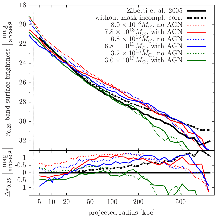
Figure 7: BCG+ICL surface brightness profiles of three groups simulated with and without AGN feedback are shown in the upper panel. For comparison observational constraints from Zibetti et al. (2005) obtained by stacking SDSS clusters and groups are shown. Also shown is the mean surface brightness profile they find without correcting for incomplete masking of satellite galaxies (assuming a constant fraction of $\sim 15\%$ of unmasked galaxy light). For each simulated halo, the mass $M_{200}^{\textrm{mean}}$ is given in the figure’s legend. The two groups shown in red and blue have masses very similar to the mean halo mass in Zibetti et al. (2005). The lower panel shows the difference to the profile obtained in Zibetti et al. (2005). The vertical dotted line indicates the gravitational softening.

Fig. 7 compares the surface brightness profiles of the BCG+ICL component in three of our simulated groups to observational constraints from Zibetti et al. (2005). For our simulated halos they were calculated for simulation outputs at redshift $z=0.21$ of runs with and without AGN, scaled to the reference redshift of 0.25. The profile from Zibetti et al. (2005) is a mean surface brightness profile obtained by stacking SDSS cluster and group images, with a mean halo mass of $M^{\text{mean}}_{200}\approx 7-8\times 10^{13}M_{\odot}$. Also shown is the profile they obtain without assuming a correction for incompletely masked satellite galaxies. In the figure, we compare with the two simulated groups from our sample whose mass $M^{\text{mean}}_{200}$ is closest to the mean mass of the observational sample. The mass of each simulated group is indicated in the figure’s legend. Due to the removal of gas by AGN heating, the mass in the runs with AGN is typically slightly lower. In addition, we include results for a further, lower mass group.

Without AGN, the surface brightness is typically too high in the central regions. In other words, the BCGs are overluminous in such simulations. When AGN are included, the central profile of one of the two groups, whose mass is close to the mean mass of the stacked clusters and groups, agrees very well with the observed central profile, indicating that a realistic BCG is formed in this simulation. The other massive group shown in the plot has a somewhat flatter central profile. However, given that there is object-to-object scatter, no perfect agreement for all halos close to the mean mass is expected.

At radii larger than about 30 kpc, the surface brightness of the two more massive simulated groups exceeds the observed profile by roughly $\sim 1\,\textrm{mag}/\textrm{arcsec}^{2}$ or somewhat less when AGN are included. This is consistent with our previous findings that we have a very significant ICL component in our simulated halos, which as this comparison confirms appears to exceed the observed amount of ICL. As illustrated further in the figure, we would need to compare to a simulated group of significantly lower mass to get a surface brightness profile that is close to the mean observed one within 200 kpc. However, in this case the simulated profile would then start to significantly underpredict the surface brightness at even larger radii. One should keep in mind though that for large radii this comparison may be quite sensitive to the accuracy of the correction for incomplete masking of satellite galaxies in Zibetti et al. (2005).

3.1.4 How do AGN affect the central cluster galaxies?

Without a strong feedback mechanism, hydrodynamical simulations of galaxy clusters suffer from excessive overcooling in cluster cores. Typically, the central galaxy is fed by a strong cooling flow and becomes too massive, too luminous and too blue compared to observations. One of the main aims of including AGN heating in cluster simulations was to offset cooling in cluster cores and produce more realistic central galaxies. Comparing the BCGs in runs with and without AGN feedback to observations should thus allow us to assess whether the employed AGN feedback model successfully regulates the central cooling flow.

Fig. 8 shows the r-band luminosities of the BCGs in our simulations as a function of cluster mass. Results are shown for runs with and without AGN feedback and are compared to observational constraints from Popesso et al. (2007). Here Method 1 was used for finding the BCGs. The AGN heating successfully reduces the BCG luminosities for all halo masses and strongly improves the agreement with observations. For massive clusters the BCG luminosities obtained with AGN are still somewhat larger than observed. However, one should note that this depends somewhat on the details of the method used for making a distinction between the BCG and ICL components in the simulations. When Method 3 or 4 is used, the resulting relation has much more scatter and the agreement with observations in runs with AGN is not as good as with Method 1 or 2. Note that the reduced BCG mass in our runs with AGN also reduces the gravitational lensing efficiency of our galaxy clusters (see Mead et al., 2010).

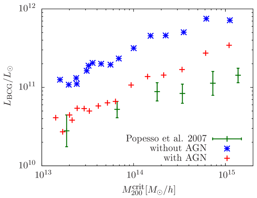
Figure 8: r-band BCG luminosity as a function of cluster mass $M_{200}^{\textrm{crit}}$. Results are shown for runs with and without AGN feedback. Method 1 (see Sect. 2.2) was used for finding the BCGs. Observational data (median BCG luminosities for six cluster mass bins) from Popesso et al. (2007) are shown for comparison. The AGN feedback significantly reduces the BCG luminosities and improves agreement with observations.

3.2 When and where do the stellar populations of satellite galaxies, BCGs, and the ICL form?

We now explore in what objects the stars have formed that are part of satellite galaxies, the BCG, and the ICL at redshift $z=0$. Using the IDs of the simulation particles, we can easily trace back every star particle in the simulation to the first snapshot after its formation. We then consider the SUBFIND (sub-)halo that the star particle is part of in this snapshot as its formation halo. Because we have saved simulation snapshots very frequently, there is only a negligibly small number of particles that are not bound to any halo in the first snapshot after their creation. We can thus, in this way, assign formation halos to almost all star particles in the simulation.

Fig. 9 shows the formation time of the star particles that are found in the BCG, the ICL, and the satellite member galaxies of a $10^{14}\,h^{-1}M_{\odot}$ cluster at $z=0$. Results are shown for simulations of this cluster with and without AGN feedback. Comparing the two runs clearly shows that AGN efficiently suppress star formation at low redshift. The effect is particularly strong for the BCG where star formation is almost completely shut off at redshifts $z<2$. It is also interesting that in the run with AGN the BCG stars form on average earlier than the stars in the satellite galaxies, which nicely agrees with the observed cosmic “down-sizing”, where the mass of galaxies hosting star formation decreases with time (e.g. Cowie et al., 1996). At first, this observational finding is counterintuitive in a hierarchical structure formation scenario. However, using semi-analytic galaxy formation models, De Lucia et al. (2006) have shown that AGN feedback allows reproducing this behaviour in a $\Lambda$CDM cosmology where structure forms hierarchically. Our results indicate that the AGN feedback model in our cosmological hydrodynamical simulations operates in the same way.

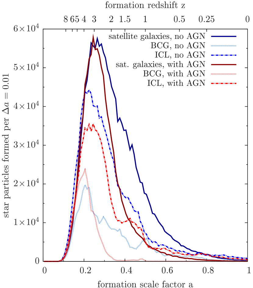
Figure 9: Distribution of the formation times of the stars in the satellite galaxies, the BCG, and the ICL of a $10^{14}\,h^{-1}M_{\odot}$ cluster. Results are shown for simulations with and without AGN feedback. Method 4 was used for making a distinction between BCG and ICL. The simulations were performed at zoom factor 3 resolution (see Table 1).

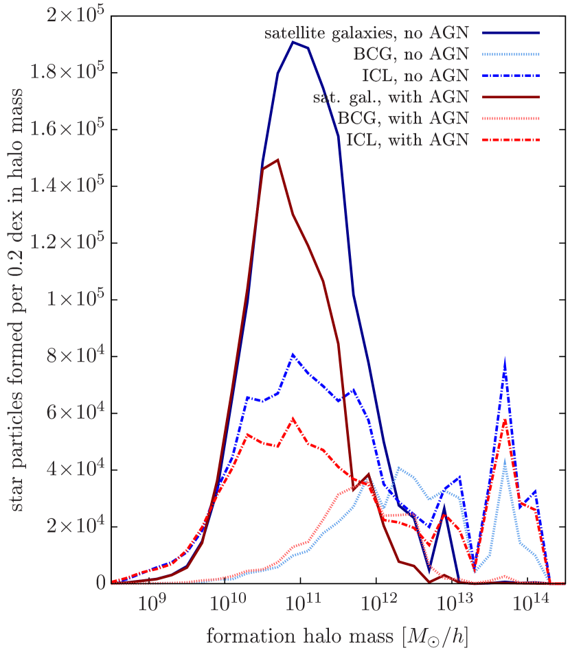
Figure 10: Distribution of the masses of the halos in which the stars in the satellite galaxies, the BCG, and the ICL of a $10^{14}\,h^{-1}M_{\odot}$ cluster formed. Results are shown for simulations with and without AGN feedback. Method 4 was used for making a distinction between BCG and ICL. The simulations were performed at zoom factor 3 resolution (see Table 1).

We also investigated in what objects stars form that at $z=0$ reside in a cluster’s satellite galaxies, in the BCG, or the ICL. Fig. 10 shows the distribution of these stars according to the mass of the halo in which they have formed. Here, the halo mass is defined as the mass of the corresponding SUBFIND (sub-)halo. For the central galaxy of a halo this is roughly the same as $M^{\text{crit}}_{200}$, but for satellite galaxies it corresponds to the smaller mass still bound within the gravitational tidal radius. The measured distributions are shown for a $M^{\text{crit}}_{200}=10^{14}\,h^{-1}M_{\odot}$ cluster and for runs with and without AGN.

Comparing the curves for the satellite galaxies, we can clearly see that AGN suppress star formation in halos larger than $\sim 5\times 10^{10}\,h^{-1}M_{\odot}$. Note that for smaller halos we do not expect any difference, as in our simulations black holes are only seeded in halos that exceed this threshold mass (see Puchwein et al., 2008). This also means that in the runs with AGN the exact shape of the distribution at the low mass end will depend on the adopted threshold for the seeding.

The stars that end up in the BCG at $z=0$ form in significantly more massive halos. This is not only due to star formation in the massive BCG itself, as for this cluster only $\sim 10\%$ and $\sim 30\%$ of the stars that reside in the BCG at $z=0$ have formed in the BCG’s main progenitor in runs with and without AGN, respectively. Instead, also the stars that are acquired during mergers with the BCG tend to be formed in more massive halos. This is not unexpected, however, since the most massive galaxies are most likely to merge with the BCG due to their shorter dynamical friction timescale. We shall return to this point in Sect. 3.3. Without AGN, there is a significant fraction of BCG stars that form in very massive halos, i.e. in halos with masses larger than $10^{13}\,h^{-1}M_{\odot}$. Indeed, many of these stars form in the cluster’s main progenitor. On the other hand, in the run with AGN, star formation is almost completely shut off in the central galaxies of such massive halos, which again demonstrates that our model for AGN feedback can efficiently suppress strong cooling flows and excessive star formation in cluster cores.

The curves for the ICL peak at roughly the same halo mass as for the satellite galaxies. However, the halo mass distribution is somewhat broader. There is also a second peak at very high halo mass, which is mostly due to stars formed in the cluster’s main progenitor. We find a similar peak for most of our simulated clusters, with a position that depends on the cluster’s mass. The occurrence of this second peak is rather surprising, especially since it is also found in runs with AGN, in which there is basically no star formation in the BCG once the cluster is as massive as required by the position of the peak. This means that these stars are not formed in the BCG but somewhere else in the cluster’s main halo.

This is illustrated for the same cluster in more detail in Fig. 11, which shows the distance of newly formed stars from the centres of their host halos. Stars that at $z=0$ are part of satellite galaxies or the BCG exclusively form in halo centres, roughly within $10\,h^{-1}{\rm kpc}$. However, a significant fraction ($\sim 30\%$) of stars that are part of the ICL at $z=0$ form at much larger distances between $10\,h^{-1}{\rm kpc}$ and $1\,h^{-1}{\rm Mpc}$. We found a similar fraction also in our other clusters.

We have investigated the nature of this ‘intracluster star formation’ in more detail, finding that it happens in small gas clouds that are distributed throughout the cluster, which can in fact be easily spotted in gas surface density maps. For most of these clouds, however, an associated halo can not be identified in maps of the dark matter particle distribution. We also checked whether these clouds form by thermal instability from the intracluster medium or whether they are stripped from infalling halos. We did this by tracing both the star-forming gas particles in these clouds, as well as all gas particles in the clusters main halo back to earlier times. This revealed that contrary to other gas particles, the vast majority of star-forming gas particles fell into the cluster very recently. For example, less than $5\%$ of the star-forming gas particles in these clouds in the progenitor of a $10^{14}\,h^{-1}M_{\odot}$ cluster at $z=1$ are already part of this progenitor’s main halo at $z=1.4$, while this fraction is over $50\%$ when looking at all main halo gas particles at the same cluster-centric radius. Also, at this earlier time most of the gas particles that later form intracluster stars can be unambiguously associated with infalling halos.

In other words, this means that most of these star-forming gas clouds consist of material that was stripped out of small infalling halos. Curiously, some of the gas clouds survived this stripping basically intact and continue to form stars, which then become part of the ICL. Note that there is observational evidence that some star formation does happen in gas stripped from infalling galaxies (e.g. Sun et al., 2010). Nevertheless, it is not entirely clear how realistic this mode of ‘intracluster star formation’ in our simulations is, and whether it is in part occurring due to numerical effects. For example, SPH simulations are known to poorly resolve fluid instabilities (e.g. Agertz et al., 2007) that could act to disrupt such gas clouds after they are stripped from an infalling halo. Also, thermal conduction in the hot intracluster medium is not included in our simulations and might play some role in reality, unless it is very efficiently suppressed by magnetic fields.

If our simulations strongly overestimate the amount of such ‘intracluster star formation’, part of the discrepancy between our simulation results and the amount of ICL inferred from observational studies like Zibetti et al. (2005) and Gonzalez et al. (2007) could be explained. In the most extreme case all star formation outside halo centres may be spurious, in which case we would expect about $\sim 30\%$ less ICL than reported above. On the other hand, it is also worth noting that if real clusters contain as many intracluster stars as predicted by our simulations, this would significantly relax the tension between constraints on the cosmic baryon fraction and baryon fractions measured in galaxy clusters as, e.g., reported in McCarthy et al. (2007). Given the difficult observational challenge to determine the amount of ICL accurately, it certainly appears possible that the present observations have still missed a significant amount of the ICL.

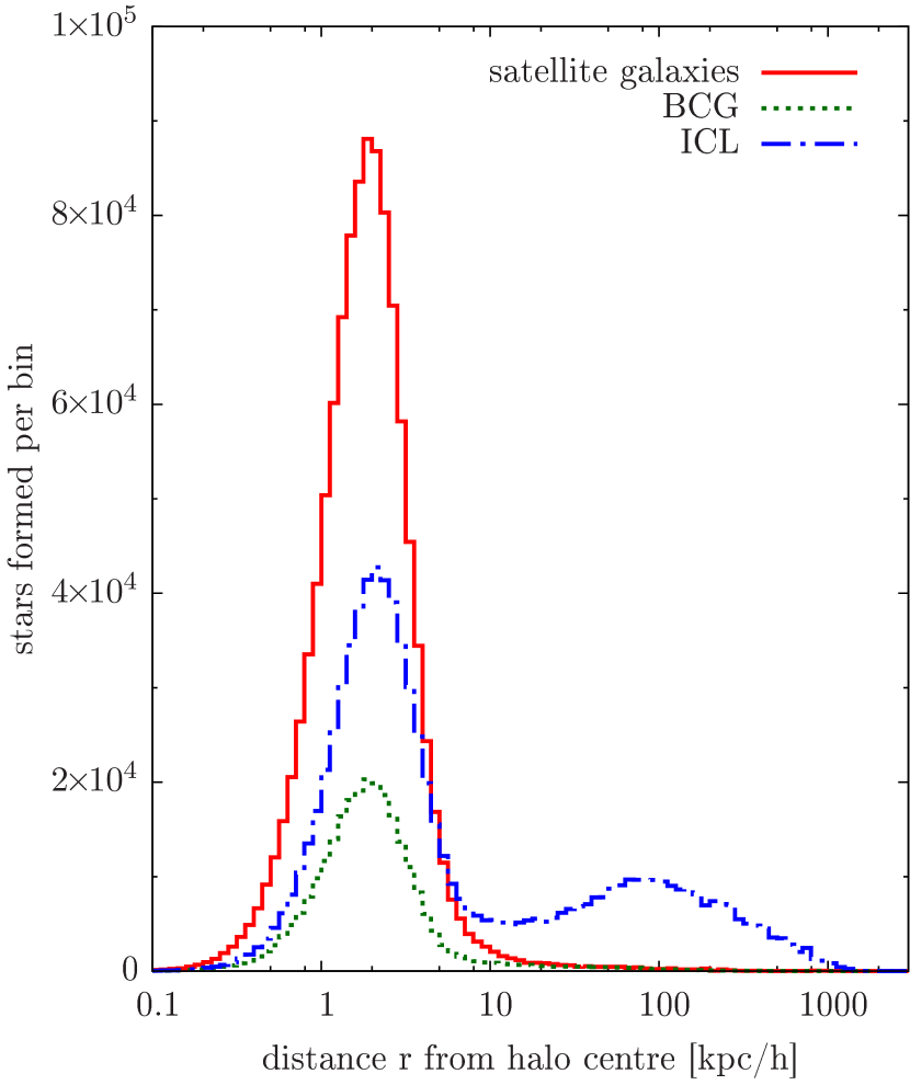
Figure 11: Distance of newly formed stars from the centres of the halos in which they were formed. Distributions are given for stars that at $z=0$ end up in satellite galaxies, the BCG, and the ICL of a $10^{14}\,h^{-1}M_{\odot}$ cluster. Method 4 was used for making a distinction between BCG and ICL. Interestingly, a significant fraction of intracluster stars is not formed in halo centres. The increase of all distributions with distance for $r$ values smaller than $\sim 1\,h^{-1}\textrm{kpc}$ is due to the increasing volume per radial bin.

3.3 In what objects do stars fall into the forming cluster?

For each star particle that was not formed in the cluster’s main progenitor we try to find the galaxy in which it fell into the forming cluster. We do this by looking for the most massive subhalo that a star particle was part of before becoming part of the main cluster’s FoF group. This allows a determination of the properties of these halos before tidal stripping in the cluster potential strongly affects them.

Fig. 12 shows the distribution of the stars in satellite galaxy, BCG, and ICL components that were not formed in the cluster’s main progenitor according to the time of their infall into the cluster. To reduce noise in the distributions we averaged them over four clusters, assigning the same weight to each of them. The simulations that were used for this figure included AGN feedback, but we note that simulations without AGN yield very similar results. The most obvious difference between the distributions is that almost all stars that end up in the BCG or ICL fall into the cluster before redshift $z\sim 1$, while the vast majority of stars that fall into the cluster later remain bound to their host galaxies. This suggests that galaxies falling into the cluster after redshift $z\sim 1$ do usually not have enough time to sink towards the cluster centre by dynamical friction and are thus unlikely to merge with the BCG or get tidally disrupted close to the centre. This further suggests that it takes a significant amount of time after the infall of a galaxy into a cluster until stars are efficiently stripped from it. Keeping this in mind, it is not at all surprising that Murante et al. (2007) find that most of the stripping happens at $z<1$.

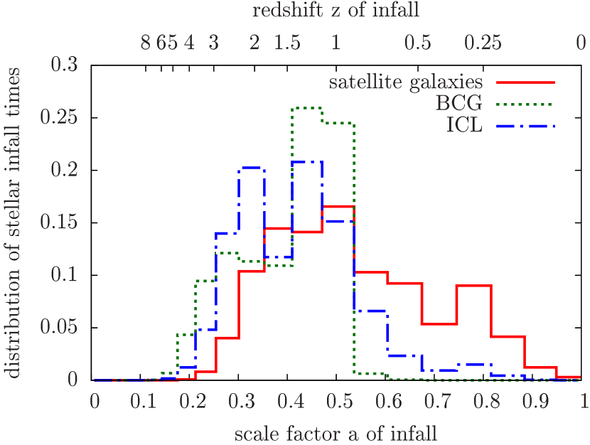
Figure 12: Distribution (fraction per bin, each histogram is normalized to unity) of stars according to the time of their infall into the forming cluster. Results are shown for stars assigned to satellite galaxies, the BCG, and the ICL at redshift $z=0$. Method 4 was used for making a distinction between BCG and ICL. All curves were averaged over four clusters that were simulated with AGN. The same weight was used for each of them.

We also checked the stellar masses of the galaxies in which the different components (satellite galaxy, BCG, and ICL stars) resided when they fell into the forming cluster. This is illustrated in Fig. 13. The lower panel shows the distribution of all infalling stars according to the stellar mass of the galaxy in which they fell into the cluster. The upper panel shows for each stellar mass bin of the infalling galaxy the fraction of stars that at $z=0$ reside in the cluster’s satellite galaxies, the BCG, and the ICL. Again, the results were averaged over four clusters to reduce noise in the curves. For stellar masses below $\sim 4\times 10^{9}\,h^{-1}M_{\odot}$, the fraction of stars that get stripped from an infalling galaxy and become intracluster stars strongly increases in our simulations. This is because these objects are poorly resolved, as also shown by our analysis of the convergence of the properties of the satellite galaxy population in Sect. 2.3. However, looking at the lower panel we see that only very few stars fall into the cluster in such small, poorly resolved galaxies. Their disruption does therefore not significantly bias our predictions for the ICL. On the other hand, for more massive and well resolved galaxies, we find that the fraction of stars that gets liberated and joins the ICL increases with the galaxy’s stellar mass. The most massive galaxies are also most likely to merge with the BCG, as can be seen by the strong increase of the BCG fraction. Accordingly, the fraction of stars that remains bound to an infalling galaxy decreases with stellar mass. This can be understood due to the shorter dynamical friction timescale for massive galaxies, while at the same time their tidal radius is larger.

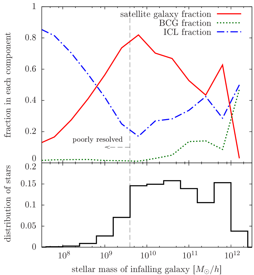
Figure 13: Distribution (fraction per bin) of stars according to the stellar mass of the galaxy in which they fell into the forming cluster (lower panel). The upper panel shows for each stellar mass bin of the infalling galaxies the fraction of stars that end up in satellite galaxies, the BCG, and the ICL at redshift $z=0$. Method 4 was used for making a distinction between BCG and ICL. All curves were averaged over four clusters that were simulated with AGN. The same weight was used for each of them.

Furthermore, we investigated what fraction of intracluster stars comes from completely dissolved galaxies. We did this by constructing a merger tree. For each SUBFIND (sub-)halo found in one snapshot we searched for the descendant (sub-)halo in the next snapshot that contains the largest number of the object’s original star particles. In case this would yield the cluster’s main halo as descendant, we also check which subhalo of the cluster contains the largest number of the satellite galaxy’s stars. If this subhalo still contains more than $10\%$ of the original galaxy’s star particles we consider it as the descendant, and not the cluster’s main halo. This allows us to follow satellite galaxies even when they are strongly tidally stripped between two subsequent simulation snapshots.

We find that the fraction of intracluster stars that comes from dissolved galaxies, i.e. galaxies that either merged with the BCG or were completely tidally disrupted, depends on halo mass. While we have performed this analysis only for four clusters, we find a systematic trend where this fraction drops from $75\%$ for a $5\times 10^{13}\,h^{-1}M_{\odot}$ group to $22\%$ for a $3\times 10^{14}\,h^{-1}M_{\odot}$ cluster.

As discussed above, the mean fraction of stars that gets stripped from an infalling galaxy and becomes part of the ICL depends on the mass of the galaxy. On the other hand, this also means that the fraction of intracluster stars may be biased in simulations that do not reproduce the correct galaxy stellar mass function. Getting the latter right in cosmological hydrodynamical simulations is, however, a long-standing problem which has not yet been solved satisfactorily. Looking at the upper panel of Fig. 13, we see that we might overestimate the ICL fraction if we significantly overpredict the number of very low mass or very massive galaxies. The former does not seem to be a problem as indicated by the distribution in the figure’s lower panel. The abundance of massive galaxies, however, is typically overpredicted in cosmological hydrodynamical simulations (see e.g. Oppenheimer et al. (2009)). This surely is the case in our simulations without AGN, but we can not be fully sure yet whether this is completely resolved when the AGN feedback model is included. Assessing this reliably requires a high resolution simulation of a large cosmological box, which has not yet been done due to the large computational cost.

Nevertheless, from exploring the cluster galaxy mass functions of our simulated clusters, we can be confident that the problem of overpredicting massive galaxies is rather strongly alleviated in runs with AGN, as also suggested by the much lower BCG luminosities shown in Fig. 8. However, the ICL fractions in our simulations with AGN feedback are even slightly higher than in the runs without it. This suggests that overpredicting massive galaxies is not the main reason why our ICL fractions are relatively high compared to the values typically inferred from observations. This also highlights that it is really far from obvious how a large ICL fraction can be avoided in the simulations of the formation of clusters in the $\Lambda$CDM cosmology.

3.4 The fate of infalling galaxies

Fig. 14 illustrates the infall of satellite galaxies and the origin of intracluster stars for a $10^{14}\,h^{-1}M_{\odot}$ cluster. The upper left panel shows all star particles residing in the cluster’s satellite galaxies, and the BCG and ICL components at $z=0$. Here, Method 4 was used for making a distinction between BCG and ICL, and the figure illustrates the assignment of the star particles to the individual components. The upper right panel of Fig. 14 shows the same cluster at $z=1$. All star particle are still coloured according to the component which they belong to at $z=0$, allowing some insights into the assembly history of the cluster galaxy population and the origin of intracluster stars.

Looking at some of the infalling galaxies, it can be easily seen that already at $z=1$ stars that later become part of the ICL are preferentially found in the outskirts of infalling galaxies, and are therefore comparatively weakly bound to them. Furthermore, the figure shows that only the most massive infalling object (marked as A) contributes a significant number of stars to the BCG, as expected from our analysis in the previous section. Following the evolution of clusters in this way also nicely shows that galaxy mergers often create a loosely bound component of stars which is subsequently stripped when the merger remnant falls into the cluster. Unfortunately, it is a bit hard to illustrate this in a still image, but it confirms the finding of Murante et al. (2007) that mergers in the assembly history of the BCG and of other massive cluster galaxies are of critical importance for the formation of the ICL.

We now consider the fate of some infalling galaxies in more detail. For this purpose we have selected two infalling objects marked as A and B in the upper right panel of Fig. 14 and followed them to redshift $z=0$. The distribution of their stars at $z=0$ is shown in the lower panels. The core of group-sized object A has basically merged with the BCG at this point. However, even after several passages of the cluster core one can still see significant tidal features both in the distribution of stars that at $z=0$ are assigned to the BCG and the ICL. The infalling galaxy B, on the other hand, remains largely intact and becomes one of the cluster’s satellite galaxies at $z=0$. Those stars that were stripped from it form a large tidal stream extending almost over the whole cluster. These two examples illustrate that the ICL really consists of many individual tidal streams and shell-like features. Only their superposition looks like a smooth distribution of intracluster stars.

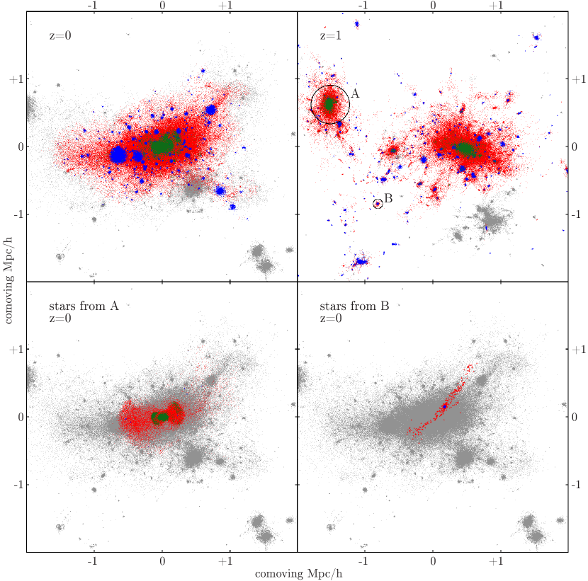
Figure 14: Distribution of stars in a $10^{14}\,h^{-1}M_{\odot}$ cluster simulated with AGN feedback. The upper left panel shows the stars residing in the cluster’s satellite galaxies (blue), BCG (green), and ICL (red) at redshift $z=0$. Grey dots indicate stars that are not part of the clusters FoF group at $z=0$. Method 4 was used for making a distinction between BCG and ICL. The upper right panel shows the cluster’s progenitors at $z=1$. All star particles are coloured as before, i.e. according to the component in which they end up at $z=0$. The circles mark two infalling objects A and B. In the lower panels the positions of the stars that are part of A (lower left) and B (lower right) at $z=1$ are shown at $z=0$. Again they are coloured according to the component to which they are assigned at $z=0$. All stars that are not part of A or B are show in grey in the lower panels.

As discussed above, stars that later become part of the ICL are preferentially found in the outskirts of infalling galaxies (see also the upper right panel of Fig. 14). It also seems plausible that the most weakly bound stars are the ones most likely to be stripped from an infalling galaxy and to become intracluster stars. We have checked this explicitly by calculating the binding energy of stars in such infalling galaxies, and Fig. 15 illustrates the results of our analysis. We show the fraction of stars that at $z=0$ reside in the cluster’s satellite galaxies, the BCG, and the ICL as a function of their binding energy in objects A and B at $z=1$. As expected, the fraction of stars that become part of the ICL strongly decreases with increasing binding energy. For object A, the most bound stars end up in the cluster’s central galaxy, while for object B, the most bound stars remain bound together in a satellite galaxy. Overall, about half of the stars in A end up in the BCG, while the other half becomes part of the ICL. For object B, only about $\sim 10\%$ of the stars are stripped and become intracluster stars.

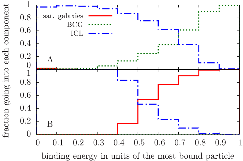
Figure 15: Distribution of binding energies in their host halos at $z=1$ of the stars that end up the cluster’s satellite galaxies, BCG, and ICL at $z=0$. Results are shown for the stars that are part of the objects A (upper panel) and B (lower panel) indicated in Fig. 14. Method 4 was used for making a distinction between BCG and ICL.

We have shown in Fig. 13 that the fraction of stars that gets stripped from an infalling galaxy depends on the galaxy’s mass. However, it also depends on the orbit of the galaxy. This is illustrated in Fig. 16, which shows the fraction of stars that at $z=0$ are still bound to a satellite galaxy as a function of the minimum distance of the galaxy’s orbit from the cluster centre. The fractions are shown for all galaxies that fell into the progenitor of a $3\times 10^{14}\,h^{-1}M_{\odot}$ cluster between redshifts $z=1.5$ and $z=1$. In order to determine the minimum distance, the orbit of the galaxy and of the cluster centre were interpolated using all simulation snapshots between the time of the galaxy’s infall and $z=0$, using a cubic interpolation between each pair of successive snapshots based on the halo positions and velocities determined by SUBFIND. The results are shown for three different stellar mass ranges of the infalling galaxy. We see that only few stars are stripped from galaxies that never come close to the cluster centre. On the other hand, galaxies that closely approach the cluster centre are often substantially stripped, completely tidally disrupted, or merge with the BCG. This confirms the expectation that most of the tidal interactions that liberate intracluster stars happen close to the cluster centre and the BCG.

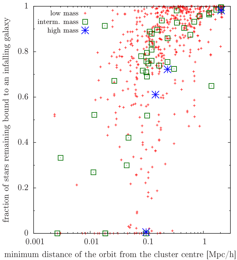
Figure 16: Fraction of stars that remain bound to a satellite galaxy as a function of the minimum distance of its orbit from the cluster centre. All galaxies that fell into the main progenitor of a $3\times 10^{14}\,h^{-1}M_{\odot}$ cluster between redshift $z=1.5$ and $z=1$ are plotted. The minimum distance was found by interpolating the galaxy’s orbit based on all simulation snapshots between the time of the infall and $z=0$. Different symbols are used for low mass galaxies (stellar mass before infall into the cluster $M_{*}$ in the range $5\times 10^{9}\,h^{-1}M_{\odot}\leq M_{*}<5\times 10^{10}\,h^{-1}M_{\odot}$), intermediate mass galaxies ($5\times 10^{10}\,h^{-1}M_{\odot}\leq M_{*}<5\times 10^{11}\,h^{-1}M_{\odot}$) and high mass galaxies ($M_{*}\geq 5\times 10^{11}\,h^{-1}M_{\odot}$). Galaxies with a fraction of 0 have either merged with the BCG or have been completely tidally disrupted.

4 Summary and conclusions

The intracluster light in clusters of galaxies represents an interesting and significant component of their total stellar mass. While the observational constraints on the ICL are still uncertain, some studies have reported intracluster star fractions of up to $\sim 50\%$. Even if the true fraction is significantly lower, it is therefore clear that the ICL can not be neglected in the baryon and stellar mass budgets of clusters. Furthermore, the radial profile of the ICL and the mass contained in it may pose interesting constraints on galaxy cluster formation models. Yet, comparatively little theoretical work has been carried out thus far on the formation of the ICL. In fact, most semi-analytic models of galaxy formation have hitherto ignored this component entirely.

In this work we have therefore studied the origin of intracluster stars in a set of high-resolution hydrodynamical simulations of the formation of clusters of galaxies, embedded in their appropriate cosmological setting. Our sample of resimulations has been randomly drawn from the Millennium simulation, with the only selection criterion being to provide a wide coverage of group and cluster masses, of roughly two orders of magnitude in halo mass. Thanks to the very high mass and force resolution of our resimulations, our simulations provide a powerful and representative sample of the whole cluster population. Another very timely aspect of our simulations is that we not only account for hydrodynamics, radiative cooling, heating by a UV background, star formation and supernovae feedback, but also incorporate a state-of-the-art model for the growth of supermassive black holes and for feedback from AGN. Because we simulated each cluster both with and without AGN physics, this allows us to pinpoint the impact of AGN heating on the cluster galaxy populations, and in particular on the ICL.

Our results clearly confirm the importance of AGN feedback in galaxy clusters. AGN lead to a reduction of the amount of stars in our clusters and groups by about one third, roughly independent of cluster mass. Especially the stellar masses and luminosities of BCGs are greatly reduced by AGN feedback, and their stellar populations become much older. As a consequence, the BCGs are in much better agreement with observational constraints. Furthermore, in poor clusters and groups, the total baryon fractions within $r^{\text{crit}}_{500}$ become significantly lower when AGN heating is included.

The primary focus of our analysis has been on the amount and the origin of the ICL component in our simulated groups and clusters. In order to allow a meaningful comparison of our simulation results with observations of clusters and groups, it was necessary to find a robust way to assign star particles in the simulations either to one of the cluster’s satellite galaxies, to the BCG, or to the ICL. Especially the distinction between the latter two components is not without ambiguities. We therefore developed and tested several different methods for distinguishing between the different components. This helps to assess the robustness of the measurements and allows the validation of measurement techniques that are close to the methods usually employed in observational studies.

Our investigation of the properties of the satellite galaxy populations, the BCGs and the ICL components in our simulations yielded the following main results:

• We find a very significant fraction of $\sim 40\%$ (without AGN) or $\sim 45\%$ (with AGN) of intracluster stars within $r^{\text{crit}}_{200}$ in our simulated clusters and groups. These values are robust with respect to numerical resolution and integration accuracy, and are almost independent of halo mass. They are, however, larger than those typically inferred from observations.

• For all the different methods we tested for making a distinction between BCG and ICL, we find that the vast majority of stars in the main halo of our simulated clusters are part of the ICL, rather than the BCG. As a result of this dominance, our ICL fractions also do not strongly depend on the exact method used for making the distinction.

• The intracluster stars form on average earlier than the stars residing in cluster satellite galaxies. Stars ending up in the BCG at $z=0$, however, typically form at even earlier times, especially when AGN are included in the simulations, which prevent excessive star formation in BCGs at low redshift.

• The fraction of stars that is stripped from infalling galaxies increases with galaxy stellar mass, which can be understood as a consequence of their larger ratio of size to tidal radius. The orbit of an infalling galaxy also plays an important role. Galaxies that closely approach the cluster centre typically loose the largest fraction of stars.

• We find that most intracluster stars are stripped from galaxies that fell into the cluster early, roughly before $z\sim 1$. Most likely, galaxies falling in later just do not have enough time to sink towards the cluster centre by dynamical friction and to get tidally disrupted there.

• The stars stripped from individual galaxies are not smoothly distributed within the cluster even after several orbits of their former host galaxy, instead they form streams and other tidal features. The ICL is therefore not smooth but a superposition of many such tidal features.

• In our simulations, a significant fraction of intracluster stars (up to $\sim 30\%$) do not form in galaxies but in cold gas clouds stripped from infalling substructures. These clouds remain intact after being stripped and give rise to ‘intracluster star formation’.

• When including AGN, the total stellar masses in our simulated galaxy groups are in good agreement with observations. However, the simulations do not reproduce the steep observed decline of the stellar mass fraction with halo mass, so that our massive simulated clusters contain more stars than suggested by observations.

It will be very interesting to see whether improved observational determinations of the ICL fraction in clusters confirm a lower value than found in our simulations. This would represent a non-trivial challenge for future simulation models, as our work has shown that the simulated ICL fraction is remarkably robust, not only with respect to integration parameters and numerical resolution, but also to quite drastic changes in the modelling of star formation. This also means that it is not obvious at all how a cluster simulation could be obtained that reproduces the galaxy population as well as in our best runs but at the same time yields a much lower ICL component.

One interesting effect we found in our simulations is that a sizable fraction of our intracluster stars actually forms ‘in situ’, in gas clouds that were stripped out of the dark matter halos of infalling galaxies but that are not bound to a dark matter satellite any more. It is not entirely clear whether this mode of ‘intracluster star formation’ is significantly affected by numerical inaccuracies in the simulations. For example, fluid instabilities might be able to disrupt these clouds and suppress the star formation in them if they are better resolved than possible with SPH. If this were indeed the case, this could explain some part of the discrepancy. On the other hand, a high ICL fraction would actually help to relax the current tensions between constraints on the cosmic baryon fraction and the baryon fractions measured in galaxy clusters.

References

- Agertz et al. (2007) Agertz O., et al., 2007, MNRAS, 380, 963
- Baldry et al. (2008) Baldry I.K., Glazebrook K., Driver S.P., 2008, MNRAS, 388, 945
- Bernardi et al. (2007) Bernardi M., Hyde J.B., Sheth R.K., Miller C.J., Nichol R.C., 2007, AJ, 133, 1741
- Borgani et al. (2006) Borgani S., et al., 2006, MNRAS, 367, 1641
- Bruzual and Charlot (2003) Bruzual G., Charlot S., 2003, MNRAS, 344, 1000
- Cowie et al. (1996) Cowie L.L., Songaila A., Hu E.M., Cohen J.G., 1996, AJ, 112, 839
- De Lucia et al. (2006) De Lucia G., Springel V., White S.D.M., Croton D., Kauffmann G., 2006, MNRAS, 366, 499
- de Vaucouleurs (1948) de Vaucouleurs G., 1948, Annales d’Astrophysique, 11, 247
- Dolag et al. (2008) Dolag K., Borgani S., Murante G., Springel V., 2008, ArXiv e-prints: 0808.3401
- Dolag et al. (2009) Dolag K., Murante G., Borgani S., 2009, ArXiv e-prints: 0911.1129
- Giodini et al. (2009) Giodini S., et al., 2009, ApJ, 703, 982
- Gonzalez et al. (2005) Gonzalez A.H., Zabludoff A.I., Zaritsky D., 2005, ApJ, 618, 195
- Gonzalez et al. (2007) Gonzalez A.H., Zaritsky D., Zabludoff A.I., 2007, ApJ, 666, 147
- Komatsu et al. (2008) Komatsu E., et al., 2008, ArXiv e-prints: 0803.0547
- Lin and Mohr (2004) Lin Y., Mohr J.J., 2004, ApJ, 617, 879
- Lin et al. (2003) Lin Y.T., Mohr J.J., Stanford S.A., 2003, ApJ, 591, 749
- McCarthy et al. (2007) McCarthy I.G., Bower R.G., Balogh M.L., 2007, MNRAS, 377, 1457
- McCarthy et al. (2009) McCarthy I.G., et al., 2009, ArXiv e-prints: 0911.2641
- Mead et al. (2010) Mead J.M.G., King L.J., Sijacki D., Leonard A., Puchwein E., McCarthy I.G., 2010, ArXiv e-prints: 1001.2281
- Murante et al. (2007) Murante G., Giovalli M., Gerhard O., Arnaboldi M., Borgani S., Dolag K., 2007, MNRAS, 377, 2
- Murante et al. (2004) Murante G., et al., 2004, ApJ, 607, L83
- Okamoto et al. (2009) Okamoto T., Frenk C.S., Jenkins A., Theuns T., 2009, ArXiv e-prints: 0909.0265
- Oppenheimer and Davé (2006) Oppenheimer B.D., Davé R., 2006, MNRAS, 373, 1265
- Oppenheimer et al. (2009) Oppenheimer B.D., Davé R., Kereš D., Fardal M., Katz N., Kollmeier J.A., Weinberg D.H., 2009, ArXiv e-prints: 0912.0519
- Popesso et al. (2007) Popesso P., Biviano A., Böhringer H., Romaniello M., 2007, A&A, 464, 451
- Puchwein et al. (2008) Puchwein E., Sijacki D., Springel V., 2008, ApJ, 687, L53
- Schombert (1986) Schombert J.M., 1986, ApJS, 60, 603
- Sijacki et al. (2007) Sijacki D., Springel V., di Matteo T., Hernquist L., 2007, MNRAS, 380, 877
- Sommer-Larsen et al. (2005) Sommer-Larsen J., Romeo A.D., Portinari L., 2005, MNRAS, 357, 478
- Springel (2005) Springel V., 2005, MNRAS, 364, 1105
- Springel and Hernquist (2003a) Springel V., Hernquist L., 2003a, MNRAS, 339, 289
- Springel and Hernquist (2003b) Springel V., Hernquist L., 2003b, MNRAS, 339, 312
- Springel et al. (2001) Springel V., White S.D.M., Tormen G., Kauffmann G., 2001, MNRAS, 328, 726
- Springel et al. (2005a) Springel V., Di Matteo T., Hernquist L., 2005a, MNRAS, 361, 776
- Springel et al. (2005b) Springel V., et al., 2005b, Nature, 435, 629
- Sun et al. (2010) Sun M., Donahue M., Roediger E., Nulsen P.E.J., Voit G.M., Sarazin C., Forman W., Jones C., 2010, ApJ, 708, 946
- Willman et al. (2004) Willman B., Governato F., Wadsley J., Quinn T., 2004, MNRAS, 355, 159
- Zibetti et al. (2005) Zibetti S., White S.D.M., Schneider D.P., Brinkmann J., 2005, MNRAS, 358, 949