Estimation of width and inclination of a filament sheet using He II 304 Å observations by STEREO/EUVI

Zusammenfassung

The STEREO mission has been providing stereoscopic view of the filament eruptions in EUV wavelengths. The most extended view during filament eruptions is seen in He II 304 Å observations, as the filament spine appears darker and sharper. The projected filament width appears differently when viewed from different angles by STEREO satellites. Here, we present a method for estimating the width and inclination of the filament sheet using He II 304 Å observations by STEREO-A and B satellites from the two viewpoints. The width of the filament sheet, when measured from its feet to its apex, gives estimate of filament height above the chromosphere.

Filaments are vertical slabs or sheet-like plasma structures in the corona. Their typical density ($\sim 2\times 10^{-10}kg/m^{3}$) is about 200 times higher and their temperature ($\sim$7,000 K) about 200 times lower than the surrounding corona. The topology of the magnetic field in filaments is such that the material is held in equilibrium against gravity and is thermally insulated from the surroundings. There are two types of filaments, one associated with active regions and other associated with large-scale weak magnetic regions or located between them. The lifetime of the former is shorter, typically few hours to days, while the latter are quite stable lasting for days to several weeks and are called quiescent filaments. The active region filaments are denser and their heights typically reach up to 10 Mm (Schmieder, 1988), while the quiescent filaments are diffuse or less dense and reach greater heights of up to 200 Mm (Pettit, 1932; D’Azambuja, 1945; Schmieder et al., 2004, 2008). However, instabilities in the filament equilibrium sometimes lead to its eruption forming the spectacular disparition brusque (DB) (Forbes and Isenberg, 1991). Most of the DBs are associated with the CMEs (Gopalswamy et al., 2003). Mouradian and Soru-Escaut (1989) classified DBs into two categories, one due to dynamic and the other due to thermal instability and suggested that the DBs associated with CMEs are due to dynamic instability. In case of filament disappearance due to thermal instability the filament reappears after the plasma has cooled down. The determination of true filament height is an important parameter in studies related to filament eruption in order to determine the height-time profile during rapid-acceleration phase of filament eruption (Schrijver et al., 2008). The stability of prominences/filaments depends upon their so-called critical height, above which they become unstable and erupt (Filippov and Den, 2001). In order to verify the critical-height criteria for erupting prominence one needs ways of determining filament height even while filament is on-disk.

Earlier, the determination of filament height was possible only from the observations of filament at limb i.e., as a prominence. With the advent of STEREO mission (Kaiser et al., 2008), we have now ways of determining height from stereoscopic information provided by views from different angles (Gissot et al., 2008; Liewer et al., 2009; Gosain et al., 2009). The three dimensional reconstruction methods have been developed based on triangulation technique (Feng et al., 2007, 2009; Aschwanden et al., 2008, 2009; Rodriguez et al., 2009). These methods use so called “tie-pointingtechnique, where same feature is manually located in both images to reconstruct the 3D coordinates of the feature (Thompson, 2006). The technique uses “epipolar constraintto reduce 2D problem to 1D (Inhester, 2006). However, for very wide separation angles these methods present difficulty in identifying common features. Nevertheless, the stereoscopic techniques can still be used to estimate the filament height and inclination even when separation angle is large (Gosain et al., 2009).

Observationally it is known that a filament sheet is a suspended structure in the corona with its feet touching the chromosphere periodically. Here, we present a method for estimating the width and inclination of the filament sheet from its projected width seen in He II 304 Å filtergrams. The width of the filament sheet and inclination are determined using simple geometric relations under simplifying assumptions regarding the filament sheet. For an erupting filament this method gives width-time profile, giving the expansion speed of the filament sheet or flux rope. Further, the full width of the filament sheet, measured from its feet to its apex, together with inclination gives an estimate of the filament height above the chromosphere. Determining filament inclination prior to their eruptions could be useful to predict the direction in which the material could be ejected, which in some cases is highly oblique as found by Bemporad (2009) by applying triangulation method on an erupting limb prominence.

The present method supplements the triangulation method and the two methods can be used together to cross-check the results for consistency. We demonstrate this by applying the two methods to a filament observed by the two STEREO satellites, separated 52.4^∘ apart, and get consistent results. The method presented here is best applied when the STEREO separation angle is large because the apparent filament width seen by the two satellites is quite different.

In section 2 we describe the method and define the various angles and notations with the help of an illustration. In section 3 we apply our method to the STEREO observations of a filament eruption during 22 May 2008. Finally, in section 4 we discuss and conclude the results.

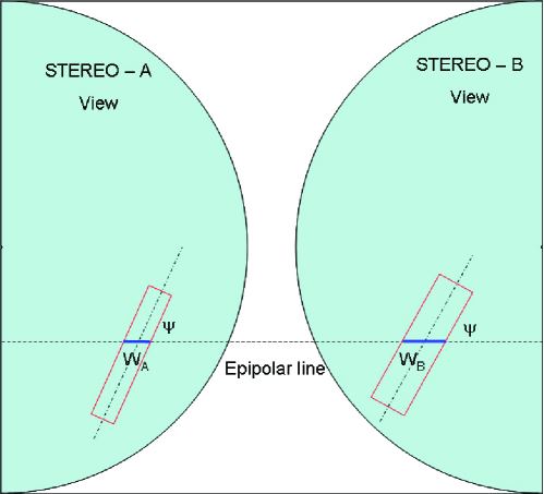
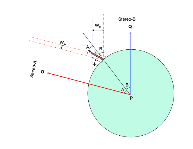
Abbildung 1: Top panel (Epipolar plane view): The two views of the sun from STEREO-A,B are illustrated with filament-axis at an arbitrary orientation $\Psi$ to epipolar plane. The projected width of the filament measured along epipolar line is $W_{A}$ and $W_{B}$. Bottom panel (Cross-sectional view) : The blue circle represents cross-section of the sun along a vertical plane through epipolar line drawn in top panel. The Sun, STEREO A, B satellites along with a cross-section of the filament along $W_{A}$ and $W_{B}$ are shown. The segment $H^{\prime}$ represents the intersection of filament sheet and epipolar plane. Since filament is oriented at an angle $\Psi$ the width of the filament sheet is determined by $H=H^{\prime}sin\Psi$. For $\Psi=90^{\circ}$ we will have $H=H^{\prime}$. The filament sheet is inclined at an angle $\gamma$ to the local solar vertical. The angles A and B are heliocentric angles of the filament base in the reference frames of STEREO-A,B respectively. P is the central point of this solar cross-section.

1 Estimation of filament inclination and width

We now present a technique for estimating the width and inclination of a filament sheet using the projected width of the filament as observed in He II 304 Å filtergrams observed by the STEREO satellites. A geometric illustration of this method is given in figure 1. The top panel of the figure 1 illustrates two views of a filament on the solar disk as seen from STEREO-A, B. The filament-axis has an arbitrary orientation $\Psi$ with respect to the epipolar line. The projected width of the filament measured along the epipolar line is $W_{A}$ and $W_{B}$. In the bottom panel of figure 1, the cross-section of the sun taken along a vertical plane passing through epipolar line (drawn in top panel) is shown. The intersection of this plane with the filament sheet can be represented by the red-hatched segment $H^{\prime}$. This segment projects widths, $W_{A}$ and $W_{B}$ towards STEREO-A and B respectively. The relation between $H^{\prime}$ and the width of the filament sheet is $H=H^{\prime}Sin\Psi$. Further, A and B are the angles subtended at point P by the filament base and central meridian longitude in the reference frames of STEREO-A, B respectively. The point P is the intersection of epipolar plane and the axis of symmetry (epipolar north-south axis). The projected width of the filament as seen by STEREO A and B is then $W_{A}=H^{\prime}sin(A-\gamma)+d\leavevmode\nobreak\ cos(A-\gamma)$ and $W_{B}=H^{\prime}sin(B+\gamma)+d\leavevmode\nobreak\ cos(B+\gamma)$, respectively. However, we can neglect the second term under the simplifying assumptions that, (i) the filament thickness $d$ is much smaller than $H^{\prime}$ i.e., ($d\ll H^{\prime}$), (ii) the STEREO separation angles $A$ and $B$ are large, and (iii) angle $A$ is not equal to $\gamma$, in which case $W_{A}$ would measure the thickness $d$ of the filament sheet. With these assumptions holding, we can attempt to measure filament inclination and width as follows:

$$\hskip 72.26999ptW_{A}=H^{\prime}sin(A-\gamma)=H^{\prime}[sinA\leavevmode\nobreak\ cos\gamma-cosA\leavevmode\nobreak\ sin\gamma]$$ (1)

$$\hskip 72.26999ptW_{B}=H^{\prime}sin(B+\gamma)=H^{\prime}[sinB\leavevmode\nobreak\ cos\gamma+cosB\leavevmode\nobreak\ sin\gamma]$$ (2)

since angles A, B and widths $W_{A}$ and $W_{B}$ are known from observations, we get using Eqns (1) and (2) above

Case 1. $\gamma<A$

$$\hskip 72.26999pttan(\gamma)=\frac{C_{1}A_{1}-C_{2}A_{2}}{C_{1}B_{2}-C_{2}B_{1}},\\$$ (3)

Case 2. $\gamma>A$

$$\hskip 72.26999pttan(\gamma)=\frac{C_{1}A_{2}-C_{2}A_{1}}{C_{1}B_{1}-C_{2}B_{2}}$$ (4)

where,

$$\leavevmode\nobreak\ \leavevmode\nobreak\ \leavevmode\nobreak\ \leavevmode\nobreak\ \leavevmode\nobreak\ \leavevmode\nobreak\ \leavevmode\nobreak\ \leavevmode\nobreak\ \leavevmode\nobreak\ \leavevmode\nobreak\ \leavevmode\nobreak\ \leavevmode\nobreak\ \leavevmode\nobreak\ \leavevmode\nobreak\ \leavevmode\nobreak\ \leavevmode\nobreak\ \hskip 72.26999ptA_{1} = sinA+sinB,$$ (5)

$$\leavevmode\nobreak\ \leavevmode\nobreak\ \leavevmode\nobreak\ \leavevmode\nobreak\ \leavevmode\nobreak\ \leavevmode\nobreak\ \leavevmode\nobreak\ \leavevmode\nobreak\ \leavevmode\nobreak\ \leavevmode\nobreak\ \leavevmode\nobreak\ \leavevmode\nobreak\ \leavevmode\nobreak\ \leavevmode\nobreak\ \leavevmode\nobreak\ \leavevmode\nobreak\ \hskip 72.26999ptB_{1} = cosA+cosB,$$ (6)

$$\leavevmode\nobreak\ \leavevmode\nobreak\ \leavevmode\nobreak\ \leavevmode\nobreak\ \leavevmode\nobreak\ \leavevmode\nobreak\ \leavevmode\nobreak\ \leavevmode\nobreak\ \leavevmode\nobreak\ \leavevmode\nobreak\ \leavevmode\nobreak\ \leavevmode\nobreak\ \leavevmode\nobreak\ \leavevmode\nobreak\ \leavevmode\nobreak\ \leavevmode\nobreak\ \hskip 72.26999ptA_{2} = sinA-sinB,$$ (7)

$$\leavevmode\nobreak\ \leavevmode\nobreak\ \leavevmode\nobreak\ \leavevmode\nobreak\ \leavevmode\nobreak\ \leavevmode\nobreak\ \leavevmode\nobreak\ \leavevmode\nobreak\ \leavevmode\nobreak\ \leavevmode\nobreak\ \leavevmode\nobreak\ \leavevmode\nobreak\ \leavevmode\nobreak\ \leavevmode\nobreak\ \leavevmode\nobreak\ \leavevmode\nobreak\ \hskip 72.26999ptB_{2} = cosA-cosB,$$ (8)

$$\leavevmode\nobreak\ \leavevmode\nobreak\ \leavevmode\nobreak\ \leavevmode\nobreak\ \leavevmode\nobreak\ \leavevmode\nobreak\ \leavevmode\nobreak\ \leavevmode\nobreak\ \leavevmode\nobreak\ \leavevmode\nobreak\ \leavevmode\nobreak\ \leavevmode\nobreak\ \leavevmode\nobreak\ \leavevmode\nobreak\ \leavevmode\nobreak\ \leavevmode\nobreak\ \hskip 72.26999ptC_{1} = W_{A}-W_{B},$$ (9)

$$\leavevmode\nobreak\ \leavevmode\nobreak\ \leavevmode\nobreak\ \leavevmode\nobreak\ \leavevmode\nobreak\ \leavevmode\nobreak\ \leavevmode\nobreak\ \leavevmode\nobreak\ \leavevmode\nobreak\ \leavevmode\nobreak\ \leavevmode\nobreak\ \leavevmode\nobreak\ \leavevmode\nobreak\ \leavevmode\nobreak\ \leavevmode\nobreak\ \leavevmode\nobreak\ \hskip 72.26999ptC_{2} = W_{A}+W_{B}$$ (10)

In order to distinguish between the two cases 1 and 2 above we can use the observation itself. In case 2, when $\gamma>A$ the filament base and surface features close-by will be seen on the same side of the spine in both STEREO A and B images, if not then case 1 holds. This is illustrated with an example in the next section, where the technique is applied on the real STEREO observations.

Thus, we can get estimate of $\gamma$ from eqn. (3) or (4) depending upon the case applicable, and then using eqn. (1) or (2) we can estimate $H^{\prime}$. The width $H$ of the filament sheet is then given by $H=H^{\prime}sin\Psi$.

2 Estimation of filament height

Let us assume that the filament is not inclined, then the height of the filament sheet is nothing but its width from its feet to its apex. For estimating the height of the filament we must, therefore, first locate the feet of the filament in the STEREO images. Then using the projected width $W_{A}$ and $W_{B}$ of the filament from its feet to the spine we can estimate the width $H$ and inclination $\gamma$ of the filament sheet using eqn. (1)-(4). We call this width as the full width $H_{f}$ (from feet to apex) of the filament sheet. The height of the filament is then given by $H_{f}cos\gamma$. This is demonstrated in the next section.

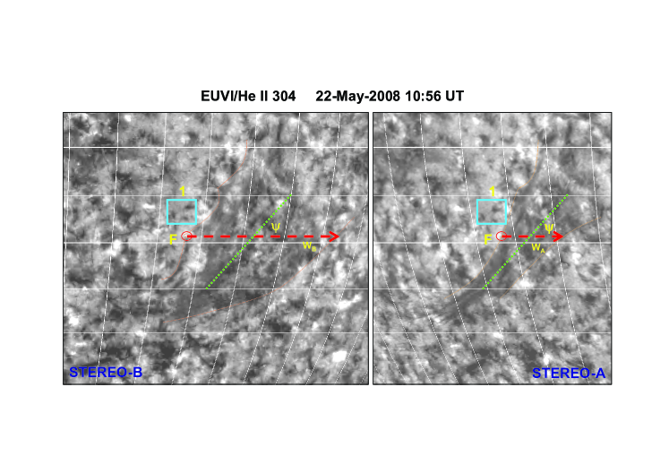
Abbildung 2: The He II 304 Å observations of a filament on 22-May-2008 during its disappearance phase at 10:56 UT. The separation angle of about 52.4 degrees between STEREO satellites shows quite different view of the filament. The spherical grid overlaid on the images help to distinguish between surface and elevated features. The location ’F’ is identified as the feet of the filament. The projected width $W_{A}$ and $W_{B}$ is marked by red arrow. Green line marks the orientation $\psi$ of the filament. Thin orange lines are drawn to demarcate the boundary of the filament. The features inside box ’1’ are surface features which are seen on left-side of the filament in both images, suggesting that the filament inclination is larger than ’A’.

Tabelle 1: Observed width and position parameters the filament.

Parameter				Value
$W_{A}$ (Mm)				79
$W_{B}$ (Mm)				194
$\angle A$ (Degrees)				31
$\angle B$ (Degrees)				20
$\Psi$ (Degrees)				48

Tabelle 2: Estimated width and inclination of the filament.

Parameter	Using apparent widths	Using SCC_MEASURE
Width, $H$ (Mm)	148	147
Inclination, $\gamma$ (Degrees)	54	47

3 Demonstration on STEREO observations

Here we apply this technique on a large filament observed by STEREO during its disappearing phase on 22 May 2008 at 10:56 UT. The STEREO images are centered, co-sized, corrected for satellite orientation to bring them in epipolar view. Figure 2 shows the filament as seen by STEREO-A and B in EUVI He II 304 Å wavelength. The filament is outlined by thin orange line. The location marked as ’F’ is inferred as feet of the filament from its arch like geometry in STEREO-B image on the left panel. Further, the surface features inside box ‘1’ are seen on left-side of the filament in both images. While this is what we expect for STEREO-B image for STEREO-A image we expect to see these features on right-side if $\gamma<A$ or beneath it (i.e., blocked by filament) if $\gamma=A$. This clearly suggests that the filament is inclined by an angle more than $A$. The horizontal red-arrow shows the segment used for determination of filament width and inclination. This segment is chosen because it extends all-the-way from the spine of the filament to its base i.e., feet marked as ‘F’. Thus, choosing this segment we can determine the full width $H_{f}$ and thus the height $H_{f}cos\gamma$ of the filament. The observed parameters of the filament for both STEREO A and B images are given in Table 1. The values of inclination angle $\gamma$ and segment $H^{\prime}$ are estimated to be 54 degrees and 200 Mm respectively. The full width, $H_{f}=H^{\prime}sin\Psi$ is thus 148 Mm and the inclination is 54 degrees. The height of the filament sheet, $H_{f}cos\gamma$, is then estimated to be 87 Mm.

These values are found to be in good agreement with the values obtained from 3D reconstructions of the same filament using SCC_MEASURE triangulation procedure as described in Gosain et al. (2009). The triangulation method SCC_MEASURE gives inclination angle $\gamma$ to be 47 degrees, while width of the sheet $H$ is found to be about 147 Mm. These values are in good agreement (Table 2) considering the simplified assumptions made in the present method. A difference of 7 degrees in the values of filament inclination determined from the two methods could be because of the finite thickness $d$ of the filament (neglected here), which would lead to excess inclination. In which case, a difference $\Delta\gamma$ of 7 degrees would mean thickness $d=H/tan(\Delta\gamma)$, which is about 18 Mm for the present case. The interesting possibility of using both the methods simultaneously to infer filament thickness $d$ along with width $H$ and inclination $\gamma$ is deferred to another study, where large number of cases will be tested for consistency. For now, one should be careful in applying the method and take into account simplifying assumptions under which estimations are made.

4 Discussion and Conclusions

When the separation angle between the twin STEREO satellites is quite large it becomes difficult to identify common features in the two images. Such identification of common features in STEREO images is quite important to compute the 3D coordinates using triangulation techniques (Inhester, 2006; Aschwanden et al., 2008). Also, the other methods like optical flow technique used by (Gissot et al., 2008) are difficult to use with widely separated angles. In such scenario our method can be used to supplement the estimates of filament width and inclination to cross-check the values obtained by other methods.

The method proposed above has obvious limitations and is applicable under simplified assumptions. These assumptions are:

(i) A filament is a rectangular sheet of thickness $d$, width $H$ and length $L$. Further, the sheet is assumed to be thin i.e., $d\ll H$. This is generally true for quiescent prominences which are very tall and thin, especially at the apex of the filament, which determines the extent of filament projection. Application to active region filaments, therefore, should not be attempted as it may give large errors.

(ii) It is possible to locate the feet of the filament in STEREO images. We demonstrated in the example presented in this paper that it is possible to carefully locate filament feet (extending down to the chromosphere). One must carefully select such portions to estimate the filament height and inclination. The height of the filament can be estimated when the projected widths $W_{A}$ and $W_{B}$ extend from filament feet to its apex. In this case the technique mentioned above would estimate inclination $\gamma$ and full width $H_{f}$ (from its feet to its apex) of the filament sheet, giving height as $H_{f}cos\gamma$.

(iii) The third assumption is that, it is possible to judge from the images whether the inclination angle gamma is larger, equal or smaller than angle A (Eq. 3 and 4). We showed using a set of STEREO observations that this is possible for a large prominence by locating position of surface features with respect to filament base. However, such determinations could be difficult in case of active region filaments which are generally low-lying and do not show wide projections.

Departure from these assumptions could lead to large errors which are not quantified yet. Especially for active region filaments, as argued above, the errors would be large. In order to quantify such errors we plan to use our technique on simulated 3D structures like extrapolated magnetic field lines in spherical geometry, in our future work.