Is Strangeness Chemically Equilibrated?

Abstract

Results related to the possible chemical equilibration of hadrons in heavy ion collisions are reviewed. Overall the evidence is very strong with a few clear and well-documented deviations, especially concerning multi-strange hadrons. Two effects are considered in some detail. Firstly, the neglect of (possibly an infinite number) of heavy resonances is investigated with the help of the Hagedorn model. Secondly, possible deviations from the standard statistical distributions are investigated by considering in detail results obtained using the Tsallis distribution.

1 Particle Yields

After analysing particle multiplicities for two decades a remarkably simple picture has emerged for the chemical freeze-out parameters [1, 2, 3]. Despite much initial skepticism, the thermal model has emerged as a reliable guide for particle multiplicities in heavy ion collisions at all collision energies. Some of the results, including analyses from [4, 5, 6, 7], are summarised in Fig. 1. Most of the points in Fig. 1 (except obviously the ones at RHIC) refer to integrated ($4\pi$) yields. A clear discrepancy exists in the lower AGS beam energy region between the (published) mid-rapidity yields and estimates of the $4\pi$ yields. The latter tend to give higher values for the chemical freeze-out temperature. This will have to be resolved by future experiments at e.g. NICA and FAIR.

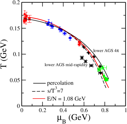
Figure 1: Values of the freeze-out parameters obtained at beam energies ranging from 1 GeV to 200 GeV

When the temperature and baryon chemical potential are translated to net baryon and energy densities, a different, but equivalent, picture emerges shown in Fig. 2. This clearly shows the importance in going to the beam energy region of around 8 - 12 GeV as this corresponds to the highest freeze-out baryonic density and to a rapid change in thermodynamic parameters [8, 9].

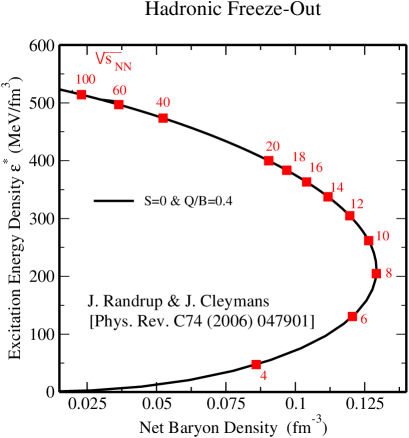
Figure 2: The hadronic freeze-out line in the $\rho_{B}-\epsilon^{*}$ phase plane as obtained from the values of $\mu_{B}$ and $T$ that have been extracted from the experimental data in [3]. The calculation employs values of $\mu_{Q}$ and $\mu_{S}$ that ensure $\langle S\rangle=0$ and $\langle Q\rangle=0.4\langle B\rangle$ for each value of $\mu_{B}$. Also indicated are the beam energies (in GeV/N) for which the particular freeze-out conditions are expected at either RHIC or FAIR or NICA.

The dependence of $\mu_{B}$ on the invariant beam energy, $\sqrt{s_{NN}}$, can be parameterized as [3]

$$\mu_{B}(\sqrt{s_{NN}})=\frac{1.308~{}\mathrm{GeV}}{1+0.273~{}{\mathrm{GeV}}^{-1}\sqrt{s_{NN}}}.$$

Similar dependences have been obtained by other groups [1, 2]. and are consistent with the above. This predicts at LHC $\mu_{B}\approx 1$ MeV.

To analyze the changes around 10 GeV use can be made of the entropy density, $s$, divided by $T^{3}$ which has been shown to reproduce the freeze-out curve [3] very well. This allows for a separation into baryonic and mesonic components, shown in Fig. 3, it can be seen that mesons dominate the chemical freeze-out from about $\sqrt{s_{NN}}\approx$ 10 GeV onwards.

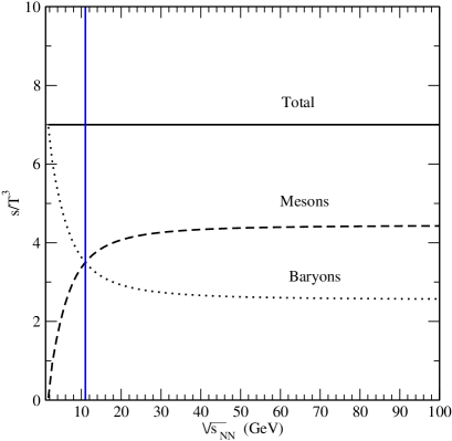
Figure 3: Values of entropy density divided by $T^{3}$ following the chemical freeze-out values.

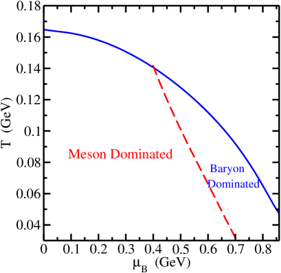
Figure 4: Regions in the $T-\mu_{B}$ plane where baryons or mesons dominate as indicated.

2 Resonance Gas and Hagedorn Spectrum

It is possible to compare analytically the resonance gas which uses a finite number of resonances up to some maximum mass, with a Hagedorn gas which contains an infinite number of resonances with an exponentially rising number of resonances as the mass increases. It is well known that at some point the Hagedorn resonance gas will show a divergence when the temperature reaches the Hagedorn value [11, 12, 13, 14].
The speed of sound is given by

$$c_{s}^{2}=\left.{\partial P\over\partial\epsilon}\right|_{s/n}$$

where the derivative is taken at a fixed entropy per particle.
For an ideal Boltzmann gas of identical scalar particles of mass $m_{0}$ and three charge states (“pions”) contained in a volume $V$, the grand partition function is defined as

$$Z(T,V)~{}=~{}{{\sum}_{N}}{\frac{1}{N!}}{\Bigg{[}\frac{3~{}V}{(2\pi)^{3}}{\int}d^{3}p\exp\{-\sqrt{p^{2}+{m_{0}}^{2}}/T\}\Bigg{]}}^{N}.$$

This expression can be evaluated, giving

$$\ln Z(T,V)~{}=~{}3{\frac{VT{m_{0}}^{2}}{2{\pi}^{2}}}K_{2}(m_{0}/T),$$

The speed of sound in this gas is given by

$$\frac{1}{c^{2}_{s}}-3~{}=~{}\frac{{m_{0}}^{2}K_{2}(m_{0}/T)}{4T^{2}K_{2}(m_{0}/T)+m_{0}TK_{1}(m_{0}/T)}$$ (1)

Now extend this to an ideal Boltzmann gas of resonances [11], described by an exponentially increasing mass spectrum of the Hagedorn form

$$\rho(m)~{}=3\delta(m-m_{0})~{}+~{}Am^{-4}\exp\{m/T_{c}\}~{}\theta(m-2m_{0}).$$ (2)

The $\theta$-function assures that the resonance spectrum starts above the two-pion threshold. The grand partition function is now given by

$$\ln Z(T,V)~{} = ~{}{VT\over 2\pi^{2}}3m_{0}^{2}K_{2}(m_{0}/T)$$ (3)

$$+ {VT\over 2\pi^{2}}A{\int}^{\infty}_{\!2m_{0}}dm~{}m^{-2}~{}\exp\{m/T_{c}\}~{}K_{2}(m/T),$$ (4)

and the speed of sound by

$$\frac{1}{c^{2}_{s}}~{}-3~{}=$$

$${3m_{0}^{4}K_{2}(m_{0}/T)~{}+~{}A\int^{\infty}_{2m_{0}}dm~{}\exp\{m/T_{c}\}~{}K_{2}(m/T)\over 2\pi^{2}Ts_{0}~{}+~{}A~{}T{\int}^{\infty}_{2m_{0}}dm~{}{m}^{-2}~{}\exp\{m/T_{c}\}~{}\left[4TK_{2}(m/T)~{}+~{}mK_{1}(m/T)\right]}.$$ (5)

The second term in the numerator diverges as $T\to T_{c}$, which in turn causes the speed of sound to vanish there [11, 12, 13].

Figure 5: Speed of sound calculated using the thermal model, following the values of the chemical freeze-out curve but with different contributions to the resonance gas determined by the masses of the resonances.

At low temperatures there is almost no difference between a Hagedorn gas and a thermal model containing only a limited number of resonances, however at higher temperatures the calculated speeds of sound become very different as shown in Fig. 5. It is thus always necessary to check if results obtained in the thermal model are stable against the addition of a Hagedorn-type of mass spectrum. Fortunately, for many quantities of interest the answer is yes [12].

3 Non-extensive Tsallis statistics

For the Tsallis distribution [15], one replaces the standard expression for the entropy based on

$$S=-\sum_{i}p_{i}\ln p_{i},$$ (6)

with

$$S_{T}={1-\sum_{i}p_{i}^{q}\over q-1}.$$ (7)

This introduces a new variable $q$, often referred to as the Tsallis parameter. In the limit where this parameter goes to 1 one recovers the Boltzmann entropy

$$\lim_{q\rightarrow 1}S_{T}=S$$ (8)

The physical interpretation of the Tsallis parameter is not obvious, we will subscribe here to the one presented in Ref. [23].

We have repeated the analysis for particle yields using the Tsallis distribution. The particle densities of particle yields were calculated using [18]:

$$n^{T}(E)=\left[1+(q-1){E-\mu\over T}\right]^{-1/(q-1)}$$ (9)

A very interesting application of this distribution to the transverse momentum distribution observed in heavy ion collisions has been presented at this conference by the STAR collaboration [20]. In the limit where the parameter $q$ tends to 1 one recovers the Boltzmann distribution:

$$\lim_{q\rightarrow 1}n^{T}(E)=\exp\left(-{E-\mu\over T}\right)$$ (10)

Figure 6: Comparison between the Boltzmann and Tsallis distributions.

A comparison between the two distributions is shown in Fig. 6 Clearly, at some value of $q$, an integral over a Tsallis distribution will no longer give a convergent result.

A possible interpretation of the Tsallis Parameter $q$ has been presented in [23]. One starts by rewriting the Tsallis distribution as a superposition of Boltzmann distributions with different temperatures, this is possible using a distribution function $g$:

$$f(E) = \left(1+\left(q-1\right)\left({E-\mu\over T}\right)\right)^{-1/(q-1)},$$

$$= \int d\left({1\over T_{B}}\right)e^{-\left(E-\mu_{B}\right)/T_{B}}g\left({1\over T_{B}}\right).$$

The precise form of the function $g$ has been given in Ref. [23]. The average temperature is then given by the $T$ parameter appearing in the Tsallis distribution:

$$\left<{1\over T_{B}}\right> = \int d\left({1\over T_{B}}\right)\left({1\over T_{B}}\right)f\left({1\over T_{B}}\right)$$ (12)

$$= {1\over T}$$ (13)

and the Tsallis parameter $q$ is the deviation around this average Boltzmann temperature,

$${\left<\left({1\over T_{B}}\right)^{2}\right>-\left<{1\over T_{B}}\right>^{2}\over\left<{1\over T_{B}}\right>^{2}}=q-1$$ (14)

Thus in the limit where $q$ goes to one, this goes to zero.

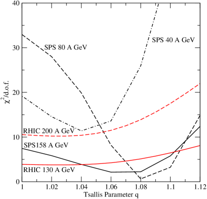
Figure 7: The $\chi^{2}$/d.o.f. of the fits as a function of the Tsallis parameter $q$.

The resulting value of $\chi^{2}$ shows an interesting dependence on the parameter $q$, as shown in Fig. 7. It must be added that most of the thermodynamic parameters show a very strong dependence on the parameter $q$ which necessitates a complete review of the physical picture behind chemical freeze-out. The temperature is shown in Fig. 8. Other variables like the volume and the chemical potential also show a strong variation with the Tsallis parameter $q$ [18].

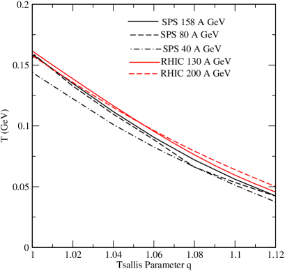
Figure 8: The freeze-out temperature as a function of the Tsallis parameter $q$.

3.1 Acknowledgments

The author acknowledges many stimulating discussions with Tamas Biro, Dan Cebra, Ingrid Kraus, Peter Levai, Helmut Oeschler, Krzysztof Redlich, Helmut Satz and Spencer Wheaton.

References

References

- [1] A. Andronic, P. Braun-Munzinger, J. Stachel, e-Print: arXiv:0911.4931 [nucl-th].
- [2] F. Becattini, J. Mannninen, M. Gazdzicki, Phys. Rev. C73 (2006) 044905.
- [3] J. Cleymans, H. Oeschler, K. Redlich, S. Wheaton Phys. Rev. C73 034905 (2006)
- [4] R. Picha, U of Davis, Ph.D. thesis 2002
- [5] J. Takahashi and R. Souza for the STAR Collaboration, e-Print: arXiv:0812.415[nucl-ex], Journal of Physics G 36 (2009) .
- [6] T. Galatyuk et al. (HADES collaboration, e-Print: arXiv:0911.2411[nucl-ex].
- [7] N. Herrmann for the FOPI collaboration, Progr. Part. Nucl. Phys. 62 (2009) 445.
- [8] J. Randrup, J. Cleymans, Phys. Rev. C74 047901 (2006).
- [9] J. Randrup, J. Cleymans, e-Print: arXiv:0905.2814 [nucl-th]
- [10] J. Cleymans, H. Oeschler, K. Redlich and S. Wheaton, Physics Letters B615 (2005) 50-54.
- [11] P. Castorina, J. Cleymans, D.E. Miller, H. Satz, e-Print: arXiv:0906.2289[hep-ph], to be published in Eur. Phys. J..
- [12] S. Chatterjee, R.M. Godbole, Sourendu Gupta, e-Print: arXiv:0906.2523[hep-ph].
- [13] J. Noronha-Hostler, H. Ahmad, J. Noronha, C. Greiner, e-Print: arXiv:0906.3960[hep-ph].
- [14] J. Noronha-Hostler, J. Noronha, C. Greiner, Phys. Rev. Lett. 103 (2009) 172302, e-Print: arXiv:0906.2523[hep-ph].
- [15] C. Tsallis, J. of Stat. Phys. 52 (1988) 479
- [16] C.E. Aguiar and T. Kodama : Physica A320 (2003) 371
- [17] T.S. Biro, G. Györgyi, A. Jakovać, G. Purcsel : J. Phys. G 31 (2005) S759
- [18] J. Cleymans, G. Hamar, P. Levai, S. Wheaton Journal of Physics G 36 (2009) 064018, hep-ph/0812.1471.
- [19] Zebo Tanh, Yichun Xu, Lijuan Ruan, Gene van Buren, Fuqiang Wang, Zhangbu Xu, Phys. Rev. C 79 (2009) 0519101
- [20] P. Sorensen, for the STAR collaboration, contribution to the proceedings of SQM2009.
- [21] T.S. Biró, K. Ürmössy, G.G. Barnaföldi, J. Phys. G 35 (2008) 044012, e-Print: arXiv:0802.0381[hep-ph].
- [22] A.M. Teweldeberhan, A.R. Plastino and H.G. Miller, Phys. Lett. A343 (2005) 71.
- [23] G. Wilk and Z. Wlodarczyk, Phys. Rev. Lett. 84 (2000) 2770.