Effect of Spin-Orbit Interaction in Spin-Triplet Superconductor: Structure of ${\bf d}$-vector and Anomalous ¹⁷O-NQR Relaxation in Sr₂RuO₄

Abstract

Supposing the spin-triplet superconducting state of Sr₂RuO₄, the spin-orbit (SO) coupling associated with relative motion in Cooper pairs is calculated by extending the method for the dipole-dipole coupling given by Leggett in the superfluid ³He. It is shown that the SO coupling works only in the equal-spin pairing (ESP) state to make the pair angular momentum $\hbar{\vec{L}}$ and the pair spin angular momentum ${\rm i}{\vec{d}}\times{\vec{d}}^{*}$ parallel with each other. The SO coupling gives rise to the internal Josephson effect in a chiral ESP state as in superfluid A-phase of ³He with a help of an additional anisotropy arising from SO coupling of atomic origin which works to direct the d-vector into $ab$-plane. This resolves the problem of the anomalous relaxation of ¹⁷O-NQR and the structure of d-vector in Sr₂RuO₄.

1 Introduction

Nature of superconductivity of Sr₂RuO₄ has attracted much attention since its discovery by Maeno and his coworkers in 1994 [1]. Now it seems to have been accepted that the Cooper pair is in the spin-triplet state [2]. However, its gap structure of the triplet state has not been confirmed yet. Especially, the intrinsic direction of the d-vector is still under debate.

The effect of spin-orbit (SO) interaction associated with relative motion of the Cooper pair, together with an atomic SO interaction and the Hund’s rule coupling, is expected to be crucial for determining the stable superconducting state among possible states in the manifold of the triplet pairing states. It will be shown that effects of SO interaction are much more crucial than that of the magnetic dipole-dipole (DD) interaction which was essential for clarifying the nature of superfluid phase of liquid ³He [3].

A highlight at earlier stages of research of Sr₂RuO₄ is a result of NMR Knight shift by Ishida et al[2] which exhibits no decrease across the transition temperature $T_{\rm c}$ when the magnetic field B of the order of Tesla is in the $ab$ (RuO₂) plane, suggesting that the Copper pairing is in the triplet state and the d-vector is in the direction parallel to the $c$-axis, perpendicular to the plane. This structure of d-vector was predicted by a group theoretical argument on the assumption that orbital and spin space are transformed together due to the “strong” SO coupling in forming the Cooper pairs [4]. However, the assumption of the “strong” SO coupling is not self-evident.

From experimental side, we should have been much more careful to draw a conclusion about the gap structure from this fact because the d-vector has a tendency to rotate in such a way that d and B are perpendicular with each other even within the $ab$-plane. Without the magnetic filed B or under the sufficiently low field, the direction of d-vector is determined by other small perturbation such as, DD or SO interaction (two-body and/or single-body), or the effect of sample boundary. The magnetic field of $\sim$Tesla seems too large to draw the conclusion about an intrinsic nature of the gap, considering the low condensation energy of $\sim k_{\rm B}T_{\rm c}$ with $T_{\rm c}\simeq 1.5$K. Concerning this subtlety, we should remember the case of UPt₃, in which the Knight shift shows no decrease for all direction of the magnetic field $B>$0.5 Tesla [5], while it shows clear decrease across $T_{\rm c}$ when $B<$0.2 Tesla is applied along $b$- or $c$-direction, suggesting the intrinsic direction of d is in the $bc$-plane [6, 7].

Indeed, six years later, Murakawa et al reported that the Knight shift does not exhibit the decrease across $T_{\rm c}$ also in the case where the small field B ($0.02<B<0.05$ Tesla) is along the $c$-axis [8, 9]. This implies that the direction of ${\bf d}$-vector identified by the former experiment is not intrinsic but is forced by the magnetic field. The most plausible interpretation of these Knight shift measurements made down to the low magnetic field of $B\sim 0.02$Tesla is that the intrinsic direction of the d-vector is in the $ab$-plane and the anisotropy field in the $ab$-plane is smaller than 0.05Tesla at most. The latter conclusion is derived from the fact that the Knight shift does not exhibit any decrease across the $T_{\rm c}$ down to the magnetic field of $B=0.05$Tesla perpendicular to the $c$-axis [9]. Therefore, theories justifying the fact that d is parallel to the $c$-axis might lose their plausibility, and other explanations are anticipated. Quite recently, it was shown that the intrinsic direction of d-vector can be in the $ab$-plane if the Coulomb interaction among electrons on the 2p orbitals of O (other than that on the 4d orbital of Ru) is taken into account[10] together with the atomic SO interaction and the Hund’s rule coupling at Ru site [11].

A role of the SO interaction between orbital and spin angular momentum of Cooper pairs may be crucial because it works to make the ${\bf d}$-vector perpendicular to L, the pair angular momentum in the $c$-axis; therefore, the d-vector is in the $ab$-plane. This effect may open a way to resolve another puzzle of anomalous NQR relaxation of ¹⁷O in the superconducting regime [12]. Indeed, the analysis shows that the dynamical spin susceptibility $\sum_{\bf q}{\rm Im}\chi_{zz}({\bf q},\omega)/\omega|_{\omega=\omega_{\rm NQR}}$ exhibits a huge enhancement at $0<T<T_{\rm c}$ while $\sum_{\bf q}{\rm Im}\chi_{xx}({\bf q},\omega)/\omega|_{\omega=\omega_{\rm NQR}}$ and $\sum_{\bf q}{\rm Im}\chi_{yy}({\bf q},\omega)/\omega|_{\omega=\omega_{\rm NQR}}$ follow the $T^{3}$-law at $0<T<T_{\rm c}$, the canonical $T$-dependence for the anisotropic superconductivity with a gap with line(s) of zero [12, 13]. A possible explanation for this behavior is that the internal Josephson effect arises through the SO coupling and gives rise to the excess NQR relaxation other than the conventional relaxation in the superconducting state due to the quasiparticles contribution. The purpose of this paper is to develop a theoretical framework to explain the effect of SO interaction of Cooper pairs in the equal-spin-pairing (ESP) state, and to resolve the puzzle of anomalous NQR relaxation observed in Sr₂RuO₄.

2 Spin-Orbit Coupling of Cooper Pairs in Triplet State

The SO interaction associated with the relative motion of quasiparticles is given as follows:

$$H_{\rm so}=-{\mu_{\rm B}^{2}\over\hbar}{m_{\rm band}\over m^{*}}\sum_{i}\sum_{j\not=i}{1\over r_{ij}^{3}}{\vec{\sigma}}_{i}\cdot\left[{\vec{r}}_{ij}\times[(2{\bar{g}}-1){\vec{p}}_{i}-2{\bar{g}}{\vec{p}}_{j}]\right],$$ (1)

where $\mu_{\rm B}$ is the Bohr magneton, $m_{\rm band}$ band mass of electron, $m^{*}$ effective mass of quasiparticles, and ${\bar{g}}$ is defined as ${\bar{g}}\equiv\mu_{\rm eff}/\mu_{\rm B}$, $\mu_{\rm eff}$ being the effective magnetic moment. The difference of prefactor of ${\vec{p}}_{i}$ from that of ${\vec{p}}_{j}$ is due to the so-called Thomas precession by the effect of the special relativity. The appearance of the factor $m_{\rm band}/m^{*}$ in (1) is due to the vertex correction for angular momentum, $m_{\rm band}/m^{*}a$, derived on an extended Ward-Pitaevskii identity as shown in Appendix [14], and that for the spin density, $1/a$ [14, 15]. The renormalization amplitude “$a$” in the denominators is cancelled by the weight of quasiparticles “$a$”.

In this paper, we restrict our discussions within the triplet manifold of ESP. By the procedure similar to that described in Ref. [3] for the dipole interaction, the interaction (1) leads to the SO free energy $F_{\rm so}$, for the Cooper pairs in the chiral state with the pair angular momentum $\hbar{\vec{L}}$, as follows:

$$F_{\rm so}=-g_{\rm so}({\rm i}{\vec{d}}\times{\vec{d}}^{*})\cdot{\vec{L}},$$ (2)

where the coefficient $g_{\rm so}$ depends on the details of the dispersion of the quasiparticles and the pairing interaction. In the spherical model of three dimensions (3d), $g_{\rm so}$ is given as

$$g_{\rm so}=g_{\rm d}{m_{\rm band}\over m^{*}}\times 4{4{\bar{g}}-1\over{\bar{g}}^{2}},$$ (3)

where $g_{\rm d}$ is the strength of the dipolar coupling in the “ESP”-superconducting state in 3d. In the cylindrical model or in two dimensions (2d), $g_{\rm so}$ is given as

$$g_{\rm so}=g_{\rm d}{m_{\rm band}\over m^{*}}\times 8{4{\bar{g}}-1\over{\bar{g}}^{2}}.$$ (4)

Hereafter, we derive expressions, (2) and (3) or (4), starting with the interaction Hamiltonian (1) which is represented in the second quantization as follows:

$$H_{\rm so} = -{\mu_{\rm B}^{2}\over\hbar}{m_{\rm band}\over m^{*}}\int\int{\rm d}{\bf r}_{1}{\rm d}{\bf r}_{2}{1\over|{\bf r}_{1}-{\bf r}_{2}|^{3}}\psi_{\alpha}^{\dagger}({\bf r}_{1})\psi_{\gamma}^{\dagger}({\bf r}_{2}){\vec{\sigma}}_{\alpha\beta}\delta_{\gamma\delta}$$ (5)

$$\qquad\qquad\cdot\left[({\vec{r}}_{1}-{\vec{r}}_{2})\times(-{\rm i}\hbar)\left((2{\bar{g}}-1){\vec{\nabla}}_{1}-2{\bar{g}}{\vec{\nabla}}_{2})\right)\right]\psi_{\delta}({\bf r}_{2})\psi_{\beta}({\bf r}_{1}).$$

By introducing the relative coordinate ${\bf r}\equiv{\bf r}_{1}-{\bf r}_{2}$, and the center of mass coordinate ${\bf R}\equiv({\bf r}_{1}+{\bf r}_{2})/2$, (5) is reduced to

$$H_{\rm so} = -{\mu_{\rm B}^{2}\over\hbar}{m_{\rm band}\over m^{*}}\int\int{\rm d}{\bf R}{\rm d}{\bf r}{1\over r^{3}}\psi_{\alpha}^{\dagger}({\bf R}+{\bf r}/2)\psi_{\gamma}^{\dagger}({\bf R}-{\bf r}/2){\vec{\sigma}}_{\alpha\beta}\delta_{\gamma\delta}$$ (6)

$$\qquad\qquad\qquad\cdot\left[{\vec{r}}\times(-{\rm i}\hbar)\left((4{\bar{g}}-1){\vec{\nabla}}_{r}-{1\over 2}{\vec{\nabla}}_{R}\right)\right]\psi_{\delta}({\bf R}-{\bf r}/2)\psi_{\beta}({\bf R}+{\bf r}/2).$$

The free energy due to the SO coupling is given by the expectation value of $H_{\rm so}$, (6). As in the case of dipole-dipole interaction [3], we rely on the following decoupling approximation:

$$\langle\psi_{\alpha}^{\dagger}({\bf R}+{\bf r}/2)\psi_{\gamma}^{\dagger}({\bf R}-{\bf r}/2)\psi_{\delta}({\bf R}-{\bf r}/2)\psi_{\beta}({\bf R}+{\bf r}/2)\rangle$$

$$\qquad\qquad\simeq\langle\psi_{\alpha}^{\dagger}({\bf R}+{\bf r}/2)\psi_{\gamma}^{\dagger}({\bf R}-{\bf r}/2)\rangle\langle\psi_{\delta}({\bf R}-{\bf r}/2)\psi_{\beta}({\bf R}+{\bf r}/2)\rangle$$

$$\qquad\qquad=\langle\psi_{\alpha}^{\dagger}({\bf r}/2)\psi_{\gamma}^{\dagger}(-{\bf r}/2)\rangle\langle\psi_{\delta}(-{\bf r}/2)\psi_{\beta}({\bf r}/2)\rangle.$$ (7)

Then, since (7) is independent of R,

$$F_{\rm so}\equiv\langle H_{\rm so}\rangle=-{\mu_{\rm B}^{2}\over\hbar}{m_{\rm band}\over m^{*}}({4\bar{g}}-1)V\int{\rm d}{\bf r}{1\over r^{3}}{\vec{\sigma}}_{\alpha\beta}\delta_{\gamma\delta}\cdot F_{\gamma\alpha}^{*}({\bf r})[{\vec{r}}\times(-{\rm i}\hbar){\vec{\nabla}}_{r})]F_{\delta\beta}({\bf r}),$$ (8)

where $V$ is the system volume and

$$F_{\delta\beta}({\bf r})\equiv\langle\psi_{\delta}({\bf r}/2)\psi_{\beta}(-{\bf r}/2)\rangle.$$ (9)

In terms of the conventional notation,

$$F_{\alpha\beta}({\bf r})={\rm i}({\vec{\sigma}}\sigma_{2})_{\alpha\beta}\cdot{\vec{F}}({\bf r}),$$ (10)

(8) is expressed as

$$F_{\rm so} = -{\mu_{\rm B}^{2}\over\hbar}{m_{\rm band}\over m^{*}}({4\bar{g}}-1)V\int{\rm d}{\bf r}{1\over r^{3}}{\sigma}^{i}_{\alpha\beta}\delta_{\gamma\delta}(\sigma_{k}\sigma_{2})^{*}_{\beta\gamma}(\sigma_{\ell}\sigma_{2})_{\beta\delta}$$ (11)

$$\qquad\qquad\qquad\qquad\qquad\qquad\qquad\qquad F_{k}^{*}({\vec{r}})[{\vec{r}}\times(-{\rm i}\hbar){\vec{\nabla}}_{r})]_{i}F_{\ell}({\bf r}).$$

With the use of the identity,

$$\sigma_{\alpha\beta}^{i}\delta_{\gamma\delta}(\sigma_{k}\sigma_{2})^{*}_{\beta\gamma}(\sigma_{\ell}\sigma_{2})_{\beta\delta}={\rm Tr}(\sigma_{2}\sigma_{k}\sigma_{i}\sigma_{\ell}\sigma_{2})=2{\rm i}\epsilon_{i\ell k},$$ (12)

(11) is reduced to

$$F_{\rm so}=-{\mu_{\rm B}^{2}\over\hbar}{m_{\rm band}\over m^{*}}2{\rm i}\epsilon_{i\ell k}({4\bar{g}}-1)V\int{\rm d}{\bf r}{1\over r^{3}}F_{k}^{*}({\bf r})[{\vec{r}}\times(-{\rm i}\hbar){\vec{\nabla}}_{r})]_{i}F_{\ell}({\bf r}).$$ (13)

Since the vector pairing amplitude $F_{\ell}$ is the eigen function of the relative angular momentum, the following relation holds:

$$[{\vec{r}}\times(-{\rm i}\hbar){\vec{\nabla}}_{r})]_{i}F_{\ell}({\bf r})=\hbar L_{i}F_{\ell}({\bf r}).$$ (14)

Then, with the use of the conventional definition of the d-vector as

$${\vec{F}}({\bf r})\equiv F({\bf r}){\vec{d}},$$ (15)

(11) is expressed as

$$F_{\rm so}=-{\mu_{\rm B}^{2}\over\hbar}{m_{\rm band}\over m^{*}}({4\bar{g}}-1)2{\rm i}\epsilon_{i\ell k}d^{*}_{k}d_{\ell}\hbar L_{i}V\int{\rm d}{\bf r}{1\over r^{3}}|F({\bf r})|^{2}.$$ (16)

Thus, the free energy due to the SO coupling is given as the following form:

$$F_{\rm so}=-g_{\rm so}({\rm i}{\vec{d}}\times{\vec{d}}^{*})\cdot{\vec{L}},$$ (17)

where the coupling constant $g_{\rm so}$ is expressed as

$$g_{\rm so}=\mu_{\rm B}^{2}{m_{\rm band}\over m^{*}}({4\bar{g}}-1)2V\int{\rm d}{\bf r}{1\over r^{3}}|F({\bf r})|^{2},$$ (18)

where the pair amplitude $F({\bf r})$ is given by its k-representation as

$$F({\bf r})=\sum_{k}e^{{\rm i}{\bf k}\cdot{\bf r}}F({\bf k}).$$ (19)

Explicit form of $F({\bf r})$ depends on the type of pairing and dimensionality of space. Let us first examine the ABM state in 3d case: Then the pairing amplitude $F({\bf r})$ is given as [3]

$$F({\vec{r}})=\Psi\int{{\rm d}{\hat{\bf k}}\over 4\pi}\sqrt{{3\over 2}}({\hat{k}}_{x}+{\rm i}{\hat{k}}_{y})e^{{\rm i}k_{\rm F}({\bf k}_{\rm F}\cdot{\bf r})}.$$ (20)

The ${\hat{\bf k}}$-integration of the part including ${\hat{k}}_{x}$ is performed as

$$\int{{\rm d}{\hat{\bf k}}\over 4\pi}{\hat{k}}_{x}e^{{\rm i}k_{\rm F}({\bf k}_{\rm F}\cdot{\bf r})}=-{\rm i}{x\over r}\left[{\cos k_{\rm F}r\over k_{\rm F}r}-{\sin k_{\rm F}r\over(k_{\rm F}r)^{2}}\right].$$ (21)

The integration of the part including ${\hat{k}}_{y}$ is performed similarly, leading to the expression for the pairing amplitude $F({\bf r})$ as follows:

$$F({\bf r})=\sqrt{{3\over 2}}\Psi{-{\rm i}x+y\over r}\left[{\cos k_{\rm F}r\over k_{\rm F}r}-{\sin k_{\rm F}r\over(k_{\rm F}r)^{2}}\right].$$ (22)

Then, substituting (22), the r-integration in (18) is performed as

$$\int{\rm d}{\bf r}{1\over r^{3}}|F({\bf r})|^{2} = 4\pi\Psi^{2}\int_{0}^{\infty}{{\rm d}r\over r}\left[{\cos k_{\rm F}r\over k_{\rm F}r}-{\sin k_{\rm F}r\over(k_{\rm F}r)^{2}}\right]^{2}$$ (23)

$$= \pi\Psi^{2},$$

where we used the formula of definite integral

$$\int_{0}^{\infty}{{\rm d}t\over t}\left[{{\cos t}\over t}-{{\sin t}\over t^{2}}\right]={1\over 4}$$ (24)

As a result, the coupling constant $g_{so}$, (18), is expressed as follows:

$$g_{\rm so}=\mu_{\rm B}^{2}{m_{\rm band}\over m^{*}}({4\bar{g}}-1)2\pi\Psi^{2}V$$ (25)

This result should be compared with that for the dipole-dipole interaction given by Leggett for the ABM state: [3]

$$g_{\rm d}={\pi\over 2}\mu_{\rm eff}^{2}\Psi^{2}={\pi\over 2}{\bar{g}}^{2}\mu_{\rm B}^{2}\Psi^{2}.$$ (26)

Therefore, the relation (3) holds. With the use of this coupling $g_{\rm d}$, the free energy due to the dipole-dipole interaction is given as[3]

$$F_{\rm d}=-{3\over 5}g_{\rm d}|({\vec{d}}\cdot{\vec{L}})|^{2}.$$ (27)

In the case of ABM state in 2d, the pair amplitude $F({\bf r})=F({\vec{\rho}})$ is given as

$$F({\vec{\rho}})=\Psi\int{{\rm d}{\hat{\bf k}}\over 2\pi}({\hat{k}}_{x}+{\rm i}{\hat{k}}_{y})e^{{\rm i}k_{\rm F}({\bf k}_{\rm F}\cdot{\vec{\rho}})},$$ (28)

where ${\vec{\rho}}=(x,y)$ is 2d vector in $xy$-plane. The ${\hat{\bf k}}$-integration for the first term in (28) is performed as follows:

$$\int{{\rm d}{\hat{\bf k}}\over 2\pi}{\hat{k}}_{x}e^{{\rm i}k_{\rm F}({\bf k}_{\rm F}\cdot{\vec{\rho}})} =-{{\rm i}\over k_{\rm F}}{\partial\over\partial x}\left(\int{{\rm d}{\hat{\bf k}}\over 2\pi}e^{{\rm i}k_{\rm F}({\bf k}_{\rm F}\cdot{\vec{\rho}})}\right)$$ (29)

$$=-{{\rm i}\over k_{\rm F}}{\partial J_{0}(k_{\rm F}\rho)\over\partial x}$$

$$=-{\rm i}{x\over\rho}J_{1}(k_{\rm F}\rho),$$

where $J_{n}(z)$ is the Bessel function of the $n$-th order. By a similar calculation for the second term in (28), the pair amplitude (28) is given as

$$F({\vec{\rho}})=\Psi{-{\rm i}x+y\over\rho}J_{1}(k_{\rm F}\rho)$$ (30)

Then, substituting (30), the r-integration in (18) is performed as follows:

$$\int{\rm d}{\bf r}{1\over r^{3}}|F({\bf r})|^{2} = \int{\rm d}{\vec{\rho}}|F({\vec{\rho}})|^{2}\int_{-\infty}^{\infty}{\rm d}z{1\over(\rho^{2}+z^{2})^{3/2}}$$ (31)

$$= 2\int{\rm d}{\vec{\rho}}{1\over\rho^{2}}|F({\vec{\rho}})|^{2}$$

$$= 4\pi\Psi^{2}\int_{0}^{\infty}{{\rm d}\rho\over\rho}[J_{1}(k_{\rm F}\rho)]^{2}$$

$$= 2\pi\Psi^{2},$$

where we have used the formula of definite integral

$$\int_{0}^{\infty}{{\rm d}t\over t}[J_{1}(t)]^{2}={1\over 2}.$$ (32)

Therefore, the coupling constant $g_{\rm so}$, (18), is expressed as

$$g_{\rm so}=\mu_{\rm B}^{2}{m_{\rm band}\over m^{*}}({4\bar{g}}-1)4\pi\Psi^{2}V,$$ (33)

leading to the relation (4).

In the case of 2d system Sr₂RuO₄, the free energy of dipole-dipole interaction is given as follows[16]:

$$F_{\rm d}=-{3c\over 4a\pi}g_{\rm d}\left[({\vec{d}}\cdot{\vec{L}})^{2}-{1\over 3}\right],$$ (34)

where $a$(=3.87Å) and $c$(=6.37Å) are the lattice constant of the primitive cell of Sr₂RuO₄ [17].

3 Non-Unitary State due to Spin-Orbit Coupling

The SO coupling (17) induces the non-unitary component of d-vector in general. The deviation from the structure of unitary pairing is determined by the balance of energy gain due to (17) and the loss of condensation free energy $F_{\rm cond}$. Although it is not easy to compare both effects at arbitrary temperature $0<T<T_{\rm c}$, it becomes rather easy at $T\sim T_{\rm c}$, in the so-called GL region. The $F_{\rm cond}$ in the ESP state in the GL region, is given by the GL free energy

$$F_{\rm GL}={1\over 2}\left({{\rm d}n\over{\rm d}\epsilon}\right)\left[-\left(1-{T\over T_{\rm c}}\right){\Delta_{\uparrow}^{2}+\Delta_{\downarrow}^{2}\over 2}+{7\zeta(3)\over 16}{\kappa\over(\pi k_{\rm B}T_{\rm c})^{2}}{\Delta_{\uparrow}^{4}+\Delta_{\downarrow}^{4}\over 2}\right],$$ (35)

where $({{\rm d}n/{\rm d}\epsilon})$ is the density of states (DOS) near the Fermi level of quasiparticles in the normal state, $\kappa\equiv\sum_{\bf k}|{\bf d}_{\bf k}|^{4}/(\sum_{\bf k}|{\bf d}_{\bf k}|^{2})^{2}$, and $\Delta_{{\uparrow}(\downarrow)}$ is the $\uparrow\uparrow$ ($\downarrow\downarrow$) component of the gap matrix. In the unitary state where $\Delta_{\uparrow}=\Delta_{\downarrow}=\Delta$, minimizing (35) with respect to $\Delta$, $F_{\rm cond}^{\rm unit}$ is given as follows:

$$F_{\rm cond}^{\rm unit}=-{1\over 4}\left({{\rm d}n\over{\rm d}\epsilon}\right){8\over 7\zeta(3)}{1\over\kappa}(\pi k_{\rm B}T_{\rm c})^{2}\left(1-{T\over T_{\rm c}}\right)^{2}.$$ (36)

In the GL region, the coupling $g_{\rm d}$ is given as [3]

$$g_{\rm d}={\pi\over 8}\mu_{\rm eff}^{2}\left({{\rm d}n\over{\rm d}\epsilon}\right)^{2}{8\over 7\zeta(3)}{1\over\kappa}(\pi k_{\rm B}T_{\rm c})^{2}\left[\ln(1.14\beta_{\rm c}\epsilon_{\rm c})\right]^{2}\left(1-{T\over T_{\rm c}}\right).$$ (37)

Then, considering the case of Sr₂RuO₄, we use relation (4) in 2d and obtain the ratio of $g_{\rm so}$ and $|F_{\rm cond}^{\rm unit}|$ as follows:

$${g_{\rm so}\over|F_{\rm cond}^{\rm unit}|}={m_{\rm band}\over m^{*}}{(4{\bar{g}}-1)\over{\bar{g}}^{2}}4\pi\mu_{\rm B}^{2}\left({{\rm d}n\over{\rm d}\epsilon}\right)\left[\ln(1.14\beta_{\rm c}\epsilon_{\rm c})\right]^{2}\left(1-{T\over T_{\rm c}}\right)^{-1}.$$ (38)

Let us parameterize the gap matrix as

$${\hat{\Delta}}={\Delta_{0}\over\sqrt{1+\eta^{2}}}\left(\begin{matrix}-1-\eta&0\\ 0&1-\eta\end{matrix}\right).$$ (39)

This is equivalent to represent the equilibrium value of d-vector as,

$$d_{0x}={1\over\sqrt{1+\eta^{2}}},\qquad d_{0y}={\rm i}{\eta\over\sqrt{1+\eta^{2}}},\qquad d_{0z}=0.$$ (40)

This d-vector in the equilibrium state is shown in Fig. 1. Substituting expression (39) into (35), after some standard calculations, we obtain the loss of condensation free energy $\Delta F_{\rm cond}$ as follows:

$$\Delta F_{\rm cond}=|F_{\rm cond}^{\rm unit}|{4\eta^{2}\over(1+\eta^{2})^{2}}.$$ (41)

The energy gain due to the SO coupling (17) is expressed in terms of (40) as follows:

$$F_{\rm so}=-g_{\rm so}{2\eta\over 1+\eta^{2}}.$$ (42)

Here we have assumed that the pair angular momentum ${\vec{L}}$ is along the $z$($c$)-axis since we are considering the case of Sr₂RuO₄.

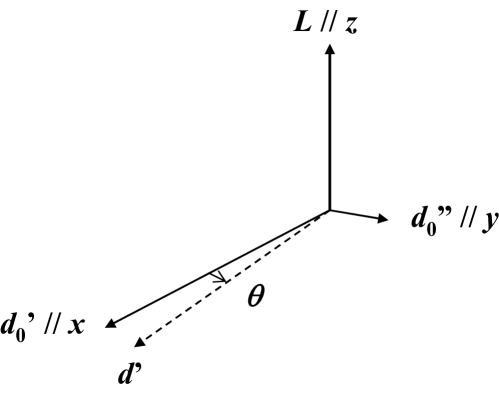
Figure 1: Structure of d-vector.

Therefore, the total free energy $F(\eta)=F_{\rm so}+\Delta F_{\rm cond}$ as a function of $\eta$ is given as

$$F(\eta)=-g_{\rm so}{2\eta\over 1+\eta^{2}}+|F_{\rm cond}^{\rm unit}|{4\eta^{2}\over(1+\eta^{2})^{2}}.$$ (43)

The degree of deviation $\eta$ from the unitary pairing is determined by the condition $\partial F(\eta)/\partial\eta=0$, which is explicitly expressed as

$$(1-\eta^{2})\left[-g_{\rm so}(1+\eta^{2})+4|F_{\rm cond}^{\rm unit}|\eta\right]=0.$$ (44)

In the case where the deviation from the unitary pairing is small, $\eta^{2}\ll 1$ can be neglected compared to unity, so that condition (44) is reduced to a simple form

$$\eta={g_{\rm so}\over 4|F_{\rm cond}^{\rm unit}|}.$$ (45)

In the case $g_{\rm so}>4|F_{\rm cond}^{\rm unit}|$, condition (44) is reduced

$$\eta=1,$$ (46)

which implies that ${\bf d}_{0}^{\prime}\perp{\bf d}_{0}^{\prime\prime}$; non-unitary state is formed.

The prefactor of $(1-T/T_{\rm c})$ in eq.(38) is estimated as

$${m_{\rm band}\over m^{*}}{(4{\bar{g}}-1)\over{\bar{g}}^{2}}4\pi\mu_{\rm B}^{2}\left({{\rm d}n\over{\rm d}\epsilon}\right)\left[\ln(1.14\beta_{\rm c}\epsilon_{\rm c})\right]^{2}\simeq 4.8\times 10^{-4}{m_{\rm band}\over m},$$ (47)

where we have used the following relations, ${\bar{g}}\simeq 1$, $({\rm d}n/{\rm d}\epsilon)=m^{*}/c\pi\hbar^{2}$, with $c=6.4$Å [17], and we have assumed $1.14\beta_{\rm c}\epsilon_{\rm c}\simeq 20$. Then, ratio (38) is estimated to be

$${g_{\rm so}\over|F_{\rm cond}^{\rm unit}|}\simeq 4.8\times 10^{-4}{m_{\rm band}\over m}\left(1-{T\over T_{\rm c}}\right)^{-1}.$$ (48)

Therefore, except for narrow temperature region near $T\simeq T_{\rm c}$, the condition $\eta^{2}\ll 1$ holds so that the relation (45) is valid. Since the energy gain due to the SO coupling is multiplied by a small factor $\eta$, (48), as in eq.(42), in order that the SO interaction predominates over the DD interaction, eq.(27), in the low-temperature region, we need another mechanism to make the ${\bf d}$ vector within the $ab$-plane, as will be discussed in the next section.

The temperature region where the effect of SO interaction predominates over the DD interaction is severely restricted near $T_{\rm c}$ as $(1-T/T_{\rm c})<10^{-3}$, taking into account the relations eqs.(26), (33), (34), (42), (45), (48), and $m_{\rm band}/m\simeq 2.9$ [17]. Therefore, it is technically impossible to observe the non-unitary state by any probe considering the broadening of the $T_{\rm c}$ itself.

4 Origin of Anisotropy of d-Vector - Anisotropy Fields

The free energy giving anisotropy of d-vector due to the magnetic fields in ESP state is expressed as [3]

$$\Delta F_{\rm magn}={1\over 2}\chi_{z}{1-Y(T)\over 1+F_{0}^{\rm a}Y(T)}({\bf d}\cdot{\bf H})^{2},$$ (49)

where $F_{0}^{\rm a}$ is the Fermi liquid parameter for the spin susceptibility; $\chi_{z}=(1+F_{0}^{a})^{-1}\mu_{\rm B}^{2}({\rm d}n/{\rm d}\epsilon)$. In the GL region, this is reduced to

$$\Delta F_{\rm magn} = {1\over\kappa}{{\displaystyle 1-{T\over T_{\rm c}}}\over 1+F_{0}^{\rm a}}\chi_{z}H^{2}$$ (50)

$$= {1\over\kappa}{{\displaystyle 1-{T\over T_{\rm c}}}\over(1+F_{0}^{\rm a})^{2}}\mu_{\rm B}^{2}\left({{\rm d}n\over{\rm d}\epsilon}\right)H^{2}.$$

This should be compared with the SO coupling constant

$$g_{\rm so}={m_{\rm band}\over m^{*}}8{(4{\bar{g}}-1)\over{\bar{g}}^{2}}{\pi\over 8}\mu_{\rm B}^{2}\left({{\rm d}n\over{\rm d}\epsilon}\right)^{2}{8\over 7\zeta(3)}{1\over\kappa}(\pi k_{\rm B}T_{\rm c})^{2}\left[\ln(1.14\beta_{\rm c}\epsilon_{\rm c})\right]^{2}\left(1-{T\over T_{\rm c}}\right),$$ (51)

where we have used relations (4) and (37). Therefore,

$${g_{\rm so}\over\Delta F_{\rm magn}}={1\over H^{2}}{m_{\rm band}\over m^{*}}(1+F_{0}^{\rm a})^{2}{8(4{\bar{g}}-1)\pi^{3}\over 7\zeta(3){\bar{g}}^{2}}\left({{\rm d}n\over{\rm d}\epsilon}\right)(k_{\rm B}T_{\rm c})^{2}\left[\ln(1.14\beta_{\rm c}\epsilon_{\rm c})\right]^{2}.$$ (52)

The actual competition between the effects of the SO coupling and the magnetic fields is given by $g_{\rm so}\eta/\Delta F_{\rm magn}$: In the region $\eta^{2}\ll 1$,

$${g_{\rm so}\eta\over\Delta F_{\rm magn}} \simeq {1\over H^{2}}(1+F_{0}^{a})^{2}{2\pi^{2}\over 7\zeta(3)}\left\{{m_{\rm band}\over m^{*}}{(4{\bar{g}}-1)\over{\bar{g}}^{2}}4\pi\mu_{\rm B}^{2}\left({{\rm d}n\over{\rm d}\epsilon}\right)\left[\ln(1.14\beta_{\rm c}\epsilon_{\rm c})\right]^{2}\right\}^{2}$$ (53)

$$\qquad\qquad\qquad\qquad\qquad\qquad\times{1\over 4}\left({k_{\rm B}T_{\rm c}\over\mu_{\rm B}}\right)^{2}\left(1-{T\over T_{\rm c}}\right)^{-1}\quad\hbox{[gauss${}^{-2}]$}$$

$$\simeq 3.0\times 10^{1}{1\over H^{2}}(1+F_{0}^{a})^{2}\left({m_{\rm band}\over m}\right)^{2}T_{\rm c}^{2}\left(1-{T\over T_{\rm c}}\right)^{-1}\quad\hbox{[gauss${}^{-2}]$},$$ (54)

where we have used the estimation (47), ${\bar{g}}\simeq 1$, $({\rm d}n/{\rm d}\epsilon)=m^{*}/c\pi\hbar^{2}$, with $c=6.37\AA$ [17], and we have assumed $1.14\beta_{\rm c}\epsilon_{\rm c}\simeq 20$. With the use of experimental values of Sr₂RuO₄, $T_{\rm c}\simeq 1.5$K, $m_{\rm band}/m\simeq 2.9$ [17], and $(1+F_{0}^{a})\simeq 0.5$ [18],

$${g_{\rm so}\eta\over\Delta F_{\rm magn}}\simeq 1.4\times 10^{2}{1\over H^{2}}\left(1-{T\over T_{\rm c}}\right)^{-1}\quad\hbox{[gauss${}^{-2}]$}.$$ (55)

Then, the anisotropy field $H_{\rm a}^{{\rm so}(2)}$ due to the two-body SO effect is given by the condition $g_{\rm so}\eta/\Delta F_{\rm magn}=1$:

$$H_{\rm a}^{{\rm so}(2)}\simeq 1.2\times 10\left(1-{T\over T_{\rm c}}\right)^{-1/2}\quad\hbox{[gauss]}.$$ (56)

In the limit of $T\to T_{\rm c}$, $\eta$ approaches 1 so that the ratio $g_{\rm so}\eta/\Delta F_{\rm magn}$ is estimated as

$${g_{\rm so}\eta\over\Delta F_{\rm magn}} \simeq 0.25\times 10^{6}{1\over H^{2}}(1+F_{0}^{a})^{2}{m_{\rm band}\over m^{*}}T_{\rm c}^{2}\quad\hbox{[gauss${}^{-2}]$}$$ (57)

$$\simeq 4.1\times 10^{5}{1\over H^{2}}\quad\hbox{[gauss${}^{-2}]$}.$$ (58)

Then, $H_{\rm a}^{\rm so(2)}$ is given as

$$H_{\rm a}^{\rm so(2)}\simeq 6.4\times 10^{2}\quad\hbox{[gauss]}.$$ (59)

The dipole-dipole interaction also gives rise to the anisotropy of d-vector [16], as discussed in superfluid ³He [3, 19] The favorite direction of d-vector is along L, relative angular momentum of Cooper pairs, i.e., $c$-axis, in contrast to the effect of the SO interaction which works to put the d-vector in the ab-plane. By the analysis similar to the above, using expressions (34), (37), and (50),

$${(3c/4a\pi)g_{\rm d}\over\Delta F_{\rm magn}}\simeq 0.39\times 10^{4}{1\over H^{2}}(1+F_{0}^{a})^{2}{m^{*}\over m}T_{\rm c}^{2}\simeq 3.6\times 10^{4}{1\over H^{2}}\quad\hbox{[gauss${}^{-2}]$},$$ (60)

where, in deriving the second relation, we have used $c/a=1.65$, $T_{\rm c}\simeq 1.5$K, $m^{*}/m\simeq 16.0$ [17], and $(1+F_{0}^{a})\simeq 0.5$ [18]. Then, the anisotropy filed $H_{\rm a}^{\rm dd}$ is estimated as

$$H_{\rm a}^{\rm dd}\simeq 1.9\times 10^{2}\quad\hbox{[gauss]}.$$ (61)

This cannot predominate over $H_{\rm a}^{\rm so(2)}$, eq.(59), in a very restricted temperature region near $T_{\rm c}$, as discussed in the last paragraph of §3. However, in the wide range of temperature $0<T<T_{\rm c}$, $H_{\rm a}^{\rm dd}$ predominates over $H_{\rm a}^{\rm so(2)}$. Therefore, the favorite direction of d-vector is the $c$-axis as far as the SO interaction and the DD interaction of Cooper pairs (both of which are two-body effect) are taken into account, which is in contradiction to the Knight shift measurements [8, 9], as discussed in the fourth paragraph of §1.

Another mechanism giving the anisotropy of the d-vetor is an atomic SO interaction (single-body effect) together with the Hund’s rule coupling [20, 21, 22]. In particular, Yanase and Ogata showed [22], on the basis of the 3rd order perturbation calculation of multiband Hubbard model for the pairing interaction [23], that the favorite direction of d-vector is the $c$-axis and the anisotropy field $H_{\rm a}^{\rm so(1)}$ due to the single-body SO interaction is of the order of $10^{-2}T_{\rm c}\sim 2\times 10^{2}$ gauss. Then, adding $H_{\rm a}^{\rm dd}$, the total anisotropy field $H_{\rm a}^{\rm total}=H_{\rm a}^{\rm dd}+H_{\rm a}^{\rm so(1)}$ amounts to $H_{\rm a}^{\rm total}\sim 4\times 10^{2}$ gauss. This is also in contradiction to the Knight shift measurements [8, 9], which shows that d-vector is perpendicular to the $c$-axis down to $H=200$ gauss.

Quite recently, however, it was shown by Yoshioka and the present author[11] that the stable direction of d-vector changes from the $c$-axis to the $ab$-plane if we take into account the Coulomb repulsion of electrons on 2p-orbitals at O site[10] which cannot be neglected as shown in a band structure calculation [24]. Indeed, the anisotropy field $H_{\rm a}^{\rm so(1)}$ is estimated as of the order of $10^{-2}T_{\rm c}$ by the calculations similar to ref.Yanase. There is a possibility that this anisotropy field wins $H_{\rm a}^{\rm dd}$, ensuring that the favorite direction of d-vector is in the $ab$-plane. Furthermore, anisotropy of d-vector is in the $ab$-plane arises through the process breaking the conservation of $z$-component of Cooper pairs by the atomic SO interaction [25]. It is noted that this process gives rise to a weak non-unitary component in the Cooper pair state.

5 Internal Josephson Oscillations

It turns out that the so-called internal Josephson effect due to the SO coupling is possible. When the d-vector in the equilibrium is given by eq.(40), its real and imaginary parts, ${\bf d}_{0}^{\prime}$ and ${\bf d}_{0}^{\prime\prime}$, are

$${\bf d}_{0}^{\prime}={1\over\sqrt{(1+\eta^{2})}}{\hat{\bf x}},\qquad{\bf d}_{0}^{\prime\prime}={\eta\over\sqrt{(1+\eta^{2})}}{\hat{\bf y}},$$ (62)

where ${\hat{\bf x}}$ and ${\hat{\bf y}}$ are the basis vector in the $x$- and $y$-directions. As the real component of d-vector, ${\bf d}_{0}^{\prime}$, deviates from equilibrium as shown in Fig. 1, the d-vector is

$${\bf d}^{\prime}={\cos\theta\over\sqrt{(1+\eta^{2})}}{\hat{\bf x}}+\sin\theta\,{\bf d}_{0}^{\prime\prime},\qquad{\bf d}^{\prime\prime}={\bf d}_{0}^{\prime\prime}.$$ (63)

Then, the diagonal components of the gap matrix are given as follows:

$$-d_{x}+{\rm i}d_{y} = {1\over\sqrt{1+\eta^{2}}}(-\cos\theta-\eta+{\rm i}\sin\theta)$$ (64)

$$= {\sqrt{1+2\eta\cos\theta+\eta^{2}}\over\sqrt{1+\eta^{2}}}{\rm exp}\left[-{\rm i}\tan^{-1}\left({\sin\theta\over\cos\theta+\eta}\right)\right],$$

and

$$d_{x}+{\rm i}d_{y}= = {1\over\sqrt{1+\eta^{2}}}(\cos\theta-\eta+{\rm i}\sin\theta)$$ (65)

$$= {\sqrt{1-2\eta\cos\theta+\eta^{2}}\over\sqrt{1+\eta^{2}}}{\rm exp}\left[{\rm i}\tan^{-1}\left({\sin\theta\over\cos\theta-\eta}\right)\right].$$

Therefore, the phase difference $\Delta\theta$ between $\uparrow\uparrow$- and $\downarrow\downarrow$-component of gap matrix is calculated as

$$\Delta\theta = \tan^{-1}\left({\sin\theta\over\cos\theta+\eta}\right)+\tan^{-1}\left({\sin\theta\over\cos\theta-\eta}\right)$$ (66)

$$= \tan^{-1}\left({\sin 2\theta\over\cos 2\theta-\eta^{2}}\right).$$

Up to the ${\cal O}(\eta^{2})$, it is approximately given by $2\theta$:

$$\Delta\theta=2\theta[1+{\cal O}(\eta^{2})].$$ (67)

For the small oscillations for which $\theta\ll 1$, the gap matrix is given up to ${\cal O}(\eta^{2})$ as follows:

$${\hat{\Delta}}=\Delta_{0}\left(\begin{matrix}(-1-\eta)e^{-{\rm i}\theta}&0\\ 0&(1+\eta)e^{{\rm i}\theta}\end{matrix}\right).$$ (68)

With the use of d-vector, eq.(63), the “pair-spin” is calculated as

$$({\rm i}{\vec{d}}\times{\vec{d}}^{*})_{z}=2({\vec{d}}^{\prime}\times{\vec{d}}^{\prime\prime})_{z}=2\eta\cos\theta.$$ (69)

Then, the free energy due to SO coupling (17) is

$$F_{\rm so}(\theta)=-g_{\rm so}(2\eta)\cos\theta,$$ (70)

where we have assumed that ${\vec{L}}={\hat{\bf z}}$ as discussed above.

The gap structure, eq.(68), and the free energy, eq.(69), have almost the same structure as those for the case of dipolar coupling in the A-phase of superfluid ³He [3]. Only difference is that $|\Delta_{\uparrow\uparrow}|$ and $|\Delta_{\downarrow\downarrow}|$ are slightly different and has weak $\theta$-dependence. Even though, the equation of motion for $\Delta\theta$ and $\Delta N\equiv N_{\uparrow}-N_{\downarrow}$, $N_{\uparrow(\downarrow)}$ being the electron number with the spin $\uparrow(\downarrow)$, are

$${{\rm d}\over{\rm d}t}(N_{\uparrow}-N_{\downarrow})=-{1\over\hbar}{\partial F_{\rm so}\over\partial(2\theta)}=-{g_{\rm so}\eta\over\hbar}\sin\theta,$$ (71)

and

$${{\rm d}\over{\rm d}t}(2\theta)=2\Delta\mu={2\mu_{\rm B}^{2}/\hbar\over\chi_{z}}(N_{\uparrow}-N_{\downarrow}).$$ (72)

These coupled equations, eqs. (71) and (72), describe the harmonic oscillations whose angular eigen frequency is given by

$$\Omega^{2} = {g_{\rm so}(\mu_{\rm B}/\hbar)^{2}\over\chi_{z}}\eta$$ (73)

$$= {g_{\rm so}(\mu_{\rm B}/\hbar)^{2}\over\chi_{z}}{g_{\rm so}\over 4|F_{\rm cond}|},$$ (74)

where expression, eq.(45), has been used for $\eta\ll 1$. With the use of eqs.(38), (51), and $\chi_{z}=(1+F_{0}^{a})^{-1}\mu_{\rm B}^{2}({\rm d}n/{\rm d}\epsilon)$, $\Omega^{2}$, eq.(74), is expressed as

$$\Omega^{2}=(1+F_{0}^{a})\left({k_{\rm B}T_{\rm c}\over\mu_{\rm B}}\right)^{2}{2\pi^{2}\over 7\zeta(3)}{1\over\kappa}\left\{{m_{\rm band}\over m^{*}}\times{(4{\bar{g}}-1)\over{\bar{g}}^{2}}4\pi\mu_{\rm B}^{2}\left({{\rm d}n\over{\rm d}\epsilon}\right)\left[\ln(1.14\beta_{\rm c}\epsilon_{\rm c})\right]^{2}\right\}^{2}.$$ (75)

Substituting eq.(47), we obtain the eigen frequency $\Omega$ as

$$\Omega\simeq 4.3\times 10^{7}\sqrt{(1+F_{0}^{a})/\kappa}\,T_{\rm c}{m_{\rm band}\over m}\quad{\hbox{[{\rm sec}${}^{-1}$]}}.$$ (76)

6 NQR Relaxation Rate due to Internal Josephson Oscillations

The dynamical uniform spin susceptibility in the A-phase in the ESP manifold has been established in the context of superfluid ³He by Leggett and Takagi as [19]:

$$\chi_{z}(\omega)=-{\Omega^{2}\chi_{z}\over\omega^{2}-\Omega^{2}+{\rm i}\Gamma\omega},$$ (77)

where the damping rate $\Gamma$ is give as

$$\Gamma=\gamma_{0}\tau\Omega^{2},$$ (78)

where $\tau$ is the lifetime of quasiparticles at normal state given as

$$\tau=b{\hbar T_{\rm F}\over k_{\rm B}T^{2}}=7.6\times 10^{-12}b{T_{\rm F}\over T^{2}},$$ (79)

where $b$ is a constant of ${\cal O}(1)$. The coefficient $\gamma_{0}$ in eq.(78) is defined as

$$\gamma_{0}\equiv[1-Y(T)]^{-1}Y(T){\chi_{z}\over{\displaystyle\mu_{\rm B}^{2}\left({{\rm d}n\over{\rm d}\epsilon}\right)}},$$ (80)

where $Y(T)$ is the Yosida function for the $p$-wave ESP state [3].

The NQR/NMR relaxation rate is given by

$${1\over T_{1}T}={A\over\mu_{\rm B}^{2}}\sum_{q<q_{\rm c}}{{\rm Im}\chi_{z}(q,\omega)\over\omega},$$ (81)

where $A$ is a constant arising from the coupling between nuclear and electron spin fluctuations. Imaginary part of $\chi_{z}(\omega)$, eq.(77), is

$${{\rm Im}\chi_{z}(\omega)\over\omega}=\chi_{z}{\gamma_{0}\tau\over{\displaystyle\left[\left({\omega\over\Omega}\right)^{2}-1\right]^{2}}+(\gamma_{0}\omega\tau)^{2}}.$$ (82)

Since expression (82) is valid for the wave number smaller than inverse of the coherence length, the size of the Cooper pair, the cut-off wave number $q_{\rm c}^{*}$ should be set as $q_{\rm c}^{*}\sim r(\pi/\xi_{0})$, where $r$ ($<$1) parameterize the cut-off size.

Then, considering the case of Sr₂RuO₄ where $\omega\simeq 1\times 10^{7}$ and eq.(76), the NQR relaxation rate due to the internal Josephson oscillations is given as

$$\left({1\over T_{1}T}\right)_{\rm S(J)}\simeq{A\over\mu_{\rm B}^{2}}\chi_{z}{\pi\over 4}n_{\rm L}cr^{2}\left({a\over\xi_{0}}\right)^{2}{\gamma_{0}\tau\over 1+(\gamma_{0}\omega\tau)^{2}},$$ (83)

where $n_{\rm L}$ is the 3d number density of lattice sites, and $n_{2d}$ is the areal number density of quasiparticles. Here, the factor $(\omega/\Omega)^{2}$ has been neglected compared to unity, because $Omega$, eq.(76), is estimated as $\sim 10^{8}\sim 10\omega$ using $(1+F^{a}_{0})\simeq 1/2$ [18], $\kappa\sim 1$, $T_{\rm c}\simeq 1.5$, and $m_{\rm band}/m\simeq 2.9$ [17]. The ratio of $\xi_{0}$ and the lattice constant $a$ in the plane is estimated as in the BCS model:

$${\xi_{0}\over a}=1.1\times 10^{-1}{T_{\rm F}\over T_{\rm c}}.$$ (84)

With the use of the experimental values, $\xi_{0}=1050$Å, and $a=3.87$Å [17], $T_{\rm F}/T_{\rm c}$ is given in turn as

$${T_{\rm F}\over T_{\rm c}}\simeq 2.5\times 10^{3}.$$ (85)

In the cylindrical or 2d model, the DOS is given as follows:

$$\left({{\rm d}n\over{\rm d}\epsilon}\right)\simeq{1\over c}{n_{2d}\over k_{\rm B}T_{\rm F}}.$$ (86)

Then, the relaxation rate, (83), due to the internal Josephson effect is expressed as

$$\left({1\over T_{1}T}\right)_{\rm S(J)}=6.5\times 10{A\over\mu_{\rm B}^{2}}{n_{\rm L}c^{2}\over n_{2d}}br^{2}\chi_{z}\hbar\left({{\rm d}n\over{\rm d}\epsilon}\right)\left({T_{\rm c}\over T}\right)^{2}{\gamma_{0}\over 1+(\gamma_{0}\omega\tau)^{2}}.$$ (87)

This expression should be compared with the Korringa relation in the normal Fermi liquid state:

$$\left({1\over T_{1}T}\right)_{\rm N} = A\sum_{\bf q}{{\rm Im}\chi_{\rm N}^{\perp}({\bf q},\omega)\over\omega}$$ (88)

$$\approx A\sum_{\bf q}{\rm Im}\left[{\chi_{0}({\bf q},\omega)\over 1+f_{0}^{a}\chi_{0}({\bf q},\omega)}\right]$$ (89)

$$\approx A{\sum_{\bf q}{\rm Im}\chi_{0}({\bf q},\omega)/\omega\over(1+F_{0}^{a})^{2}}$$ (90)

$$= A{1\over 4}{\chi_{z}\over\mu_{\rm B}^{2}}{\hbar{\displaystyle\left({{\rm d}n\over{\rm d}\epsilon}\right)}\over 1+F_{0}^{\rm a}}{q_{\rm c}\over k_{\rm F}}n_{\rm L}c^{2}a^{2},$$ (91)

where $\chi_{\rm N}^{\perp}({\bf q},\omega)$ is the transverse dynamical spin susceptibility in the normal state, $\chi_{0}({\bf q},\omega)$ is the particle-hole propagator of quasiparticles (with $\chi_{0}(0,0)={1\over 2}({\rm d}n/{\rm d}\epsilon)$, $k_{\rm F}$ is the Fermi wave number, and $q_{\rm c}\simeq 1/2\sqrt{\pi}a$ is the wave number cut-off representing the lattice effect.

In the case of Sr₂RuO₄, $\chi_{z}\simeq 2.0\times\mu_{\rm B}^{2}({\rm d}n/{\rm d}\epsilon)$ or $F_{0}^{\rm a}\simeq-0.5$ [18], $\gamma_{0}$ defined by eq.(80) is approximately given as

$$\gamma_{0}\simeq 2.0[1-Y(T)]^{-1}Y(T).$$ (92)

The parameter $\omega\tau$ in eqs. (82) and (87) is given in the present case, $\omega\simeq 1.0\times 10^{7}$ sec^-1, as

$$\omega\tau\simeq 7.6\times 10^{-5}\times b{T_{\rm F}\over T^{2}}\simeq 1.9\times 10^{-1}{b\over T_{\rm c}}\left({T_{\rm c}\over T}\right)^{2},$$ (93)

where we have used eqs. (79) and (85).

The longitudinal relaxation rate of NQR, normalized by that in the normal state, eq.(91), is

$${(1/T_{1}T)_{\rm S(J)}\over(1/T_{1}T)_{\rm N}}={6.5\times 10\over(q_{\rm c}/k_{\rm F})a^{2}n_{2d}}br^{2}4(1+F_{0}^{a})\left({T_{\rm c}\over T}\right)^{2}{\gamma_{0}\over 1+(\gamma_{0}\omega\tau)^{2}}.$$ (94)

The Yosida function $Y(T)$ in $\gamma_{0}$, eq.(92), is estimated in the standard manner by assuming that the pairing interaction $V_{{\bf k},{\bf k}^{\prime}}=-V\cos\varphi_{\bf k}\cos\varphi_{{}^{\prime}}$, $\varphi_{\bf k}$ being the azimuth in the k-space of $ab$-plane, and that the superconducting gap $\Delta_{\rm k}=\Delta\cos\varphi_{\bf k}$ follows the weak-coupling gap equation. Since, in expression (94), there exist parameters $b$ and $r$ that are difficult to estimate microscopically, we choose them so as to reproduce the observed temperature dependence of NQR relaxation rate [12]. Instead of $b$ and $r$, two independent parameters can be chosen also as

$$C\equiv{6.5\times 10\over(q_{\rm c}/k_{\rm F})a^{2}n_{2d}}br^{2},$$ (95)

and

$$D\equiv 0.39{b\over T_{\rm c}}.$$ (96)

In Fig. 2, we show the results of the NQR relaxation rate in the superconducting state, $(1/T_{1}T)_{\rm S}=(1/T_{1}T)_{\rm S(J)}+(1/T_{1}T)_{\rm S(Q)}$, where $(1/T_{1}T)_{\rm S(Q)}$ is the quasiparticles contribution and is replaced by experimental values of $(1/T_{1}T)_{b}$, for two sets of parameters, (I) $C=0.2$, $D=0.44$, and (II) $C=0.55$, $D=1.0$. Agreement of experimental measurements and the theoretical results, based on eq.(94), is rather nice, although the theoretical ones include adjustable parameters and relatively crude approximations have been done. To our best knowledge, the unusual relaxation rate $(1/T_{1}T)_{c}$ has not yet been explained. So, our theory may be the first one that explains the unusual behavior of NQR relaxation rate [12].

Figure 2: NQR relaxation rate: Comparison of experiment and theory. Filled (open) circles represent data of measurements of NQR relaxation rate due to spin fluctuations along the $c$-axis ($b$-axis) [12]. Dashed line represents $(1/T_{1}T)_{\rm S(Q)}$ due to the quasiparticles contribution which follows the $T^{3}$-law in a wide region $T<T_{\rm c}$. Solid lines (I) and (II) represent $(1/T_{1}T)_{\rm S}=(1/T_{1}T)_{\rm S(J)}+(1/T_{1}T)_{\rm S(Q)}$ for the parameter set of eqs.(95) and (96), (I) $C=0.2$, $D=0.44$, and (II) $C=0.55$, $D=1.0$, respectively.

7 Summary

We have obtained a formula for the spin-orbit coupling of the Cooper pairs in ESP state of Sr₂RuO₄, giving rise to the internal Josephson oscillations of d-vector in the $ab$-plane if the stable direction of d-vector is in the $ab$-plane. The latter condition is confirmed by a recent theoretical finding of Yoshioka and the present author[11] that the stable direction of d-vector is in the $ab$-plane on a realistic model of Sr₂RuO₄ by taking account of atomic spin-orbit interaction and the Hund’s rule coupling among electrons on 4d orbitals at Ru site. The anomalous temperature dependence of NQR relaxation rate $(1/T_{1}T)_{c}$ was explained by the theoretical formula, eq.(94), due to the internal Josephson oscillations of d-vector in the $ab$-plane that induces the oscillations of spin polarization in the direction of $c$-axis.

Appendix

In this appendix we show how the factor $m_{\rm band}/m^{*}$ appears in (1) on the basis of an extended Ward-Pitaevskii identity. Suppose the system is subject to the low rotation $\delta{\vec{\Omega}}({\bf r})$ which is slowly varying with respect to r. Then the term $-({\bf r}\times{\bf p})\cdot{\vec{\Omega}}$ is added to the Hamiltonian. Then, the variation of the Hamiltonian is given by the term

$$-\int{\rm d}{\bf r}\psi_{\alpha}^{\dagger}({\bf r})\left([{\bf r}\times{\bf p}]\cdot\delta{\vec{\Omega}}({\bf r})\right)\psi_{\alpha}({\bf r})=-\int{\rm d}{\bf r}\psi_{\alpha}^{\dagger}({\bf r})\left([\delta{\vec{\Omega}}({\bf r})\times{\bf r}]\cdot{\bf p}]\right)\psi_{\alpha}({\bf r})$$ (97)

where ${\bf p}=-{\rm i}\hbar{\vec{\nabla}}$. By this perturbation, we obtain for the variation of the Green function:

$$\delta G = -G(p)({\rm i}{\vec{\nabla}}_{p}\times{\bf p})\cdot\delta{\vec{\Omega}}G(p+k)+{{\rm i}\over 2}G(p)G(p+k)$$ (98)

$$\qquad\qquad\times\int{{\rm d}^{4}q\over(2\pi)^{4}}\Gamma_{\alpha\beta,\alpha\beta}(p,q;k)G(q)({\rm i}{\vec{\nabla}}_{q}\times{\bf q})\cdot\delta{\vec{\Omega}}G(q+k),$$

where $k=({\bf k},0)$ (we assume k to be extremely small). On the other hand, the addition of (97) to the Hamiltonian leads to the transformation of the momentum in the Green function as

$${\bf p}\rightarrow{\bf p}-m_{\rm band}\delta{\vec{\Omega}}\times({\rm i}{\vec{\nabla}}_{p}).$$ (99)

Hence,

$${\delta G\over\delta{\vec{\Omega}}}=-m_{\rm band}({\rm i}{\vec{\nabla}}_{p})\times{\partial G\over\partial{\bf p}},$$ (100)

as ${\bf k}\to 0$. Consequently, in the limit of $\delta\Omega\to 0$, and ${\bf k}\to 0$, we obtain for $G(p)$ describing the quasiparticles:

$$m_{\rm band}({\rm i}{\vec{\nabla}}_{p})\times{\partial G^{-1}\over\partial{\bf p}}=-({\rm i}{\vec{\nabla}}_{p}\times{\bf p})+{{\rm i}\over 2}\int{{\rm d}^{4}q\over(2\pi)^{4}}\Gamma^{k}_{\alpha\beta,\alpha\beta}(p,q)\{G(q)({\rm i}{\vec{\nabla}}_{q}\times{\bf q})G(q)\}_{k}.$$ (101)

Since the relation

$${\partial G^{-1}\over\partial{\bf p}}=-{{\bf v}\over a}=-{{\bf p}\over m^{*}a},$$ (102)

holds for the quasiparticles near the Fermi level, the relation (101) near the Fermi level is rephrased as

$$-{m_{\rm band}\over m^{*}a}({\rm i}{\vec{\nabla}}_{p}\times{\bf p})=-({\rm i}{\vec{\nabla}}_{p}\times{\bf p})+{{\rm i}\over 2}\int{{\rm d}^{4}q\over(2\pi)^{4}}\Gamma^{k}_{\alpha\beta,\alpha\beta}(p,q)\{G(q)({\rm i}{\vec{\nabla}}_{q}\times{\bf q})G(q)\}_{k}.$$ (103)

This explains why the vertex correction of spin-orbit coupling is given by $m_{\rm band}/m^{*}$, leading to expression (1) after the factor $1/a$ has been cancelled with the renormalization amplitude $a$ of quasiparticles.

References

• [1] Y. Maeno, H. Hashimoto, K. Yoshida, S. Nishizaki, T. Fujita, J. G. Bednorz, and F. Lichtenberg: Nature 372 (1994) 532.
• [2] K. Ishida, H. Mukuda, Y. Kitaoka, K. Asayama, Z. Q. Mao, Y. Mori and Y. Maeno: Nature 396 (1998) 658.
• [3] A. J. Leggett, Rev. Mod. Phys. 47 (1975) 331.
• [4] T. M. Rice and M. Sigrist: J. Phys.: Condens. Matter 7 (1995) L643.
• [5] H. Tou, Y. Kitaoka, K. Asayama, N. Kimura, Y. Ōnuki, E. Yamamoto, and K. Maezawa: Phys. Rev. Lett. 77 (1996) 1374.
• [6] H. Tou, Y. Kitaoka, K. Ishida, K. Asayama, N. Kimura, Y. Ōnuki, E. Yamamoto, Y. Haga, and K. Maezawa: Phys. Rev. Lett. 80 (1998) 3129.
• [7] S. Yotsuhashi, K. Miyake and H. Kusunose: Physica B 312-313 (2002) 100.
• [8] H. Murakawa, K. Ishida, K. Kitagawa, Z. Q. Mao, and Y. Maeno: Phys. Rev. Lett. 93 (2004), 167004.
• [9] H. Murakawa, K. Ishida, K. Kitagawa, H. Ikeda, Z. Q. Mao, and Y. Maeno: J. Phys. Soc. Jpn. 76 (2007) 024716.
• [10] K. Hoshihara and K. Miyake: J. Phys. Soc. Jpn. 74 (2005) 2679.
• [11] Y. Yoshioka and K. Miyake: J. Phys. Soc. Jpn. 78 (2009) 074701.
• [12] H. Mukuda, K. Ishida, Y. Kitaoka, K. Miyake, Z. Q. Mao, Y. Mori and Y. Maeno: Phys. Rev. B 65 (2002) 132507.
• [13] K. Ishida, H. Mukuda, Y. Kitaoka, Z. Q. Mao, Y. Mori, and Y. Maeno: Phys. Rev. Lett. 84 (2000) 5387.
• [14] A. A. Abrikosov, L. P. Gorkov, I. E. Dzyaloshinskii: Method of Quantum Field Theory in Statistical Physics, 2nd ed. (Pergamon Press, Oxford, 1965) Β§19.1.
• [15] A. J. Leggett: Phys. Rev. 140 (1965) A1869.
• [16] Y. Hasegawa: J. Phys. Soc. Jpn. 72 (2003) 2456.
• [17] A. P. Mackenzie, S. R. Julian, A. J. Diver, G. J. McMullan, M. P. Ray, G. G. Lonzarich, Y. Maeno, S. Nishizaki and T. Fujita, Phys. Rev. Lett. 76 (1996) 3786.
• [18] Y. Maeno, K. Yoshida, H. Hashimoto, S. Nishizaki, S. Ikeda, M. Nohara, T. Fujita, A. P. Mackenzie, N. E. Hussey, J. G. Bednorz, and F. Lichtenberg: J. Phys. Soc. Jpn. 66 (1997) 1405.
• [19] A. J. Leggett and S. Takagi: Ann. Phys. 106 (1977) 79.
• [20] K. K. Ng and M. Sigrist: Europhys. Lett. 49 (2000) 473.
• [21] M. Ogata: J. Phys. Chem. Solids 63 (2002) 1329.
• [22] Y. Yanase and M. Ogata: J. Phys. Soc. Jpn. 72 (2003) 673.
• [23] T. Nomura and K. Yamada: J. Phys. Soc. Jpn. 71 (2002) 1993.
• [24] T. Oguchi: Phys. Rev B 51 (1995) 1385.
• [25] Y. Yoshioka: private communications.