Implicit and electrostatic Particle-in-cell/Monte Carlo model in two-dimensional and axisymmetric geometry II: Self-bias voltage effects in capacitively coupled plasmas

Abstract

With an implicit Particle-in-cell/Monte Carlo model, capacitively coupled plasmas are studied in two-dimensional and axisymmetric geometry. Self-bias dc voltage effects are self-consistently considered. Due to finite length effects,the self-bias dc voltages show sophisticating relations with the electrode areas. Two-dimensional kinetic effects are also illuminated. Compare to the fluid mode, PIC/MC model is numerical-diffusion-free and thus finer properties of the plasmas are simulated.

1 Introduction

Capacitively coupled plasmas (CCP) processing is the mainstream technology for etching and deposition devices in semiconductor industry [1, 2, 3]. Besides their applications in semiconductor industry, many physical processes involved in CCP, are still not fully understood and therefore attracted many researchers, both from the academy and the industry. Except many analytical models to understand the physics in CCP qualitatively, there are two ways [4, 5] to study the plasma process in the reactors quantitatively: fluid/Monte Carlo (MC) hybrid method and Particle-in-cell/Monte Carlo (PIC/MC) method.

PIC/MC model is widely adopted in academy research because it has fewer assumptions. However, PIC/MC model is very computationally expensive. As a result, up to now, most PIC/MC simulations for CCP were only done in 1D geometry [6, 7, 8, 9, 10, 11, 12]. There are only several open reports about standard 2D simulations. Vahedi [13] presents the first 2D results based on direct implicit PIC/MC model, but in planar (X-Y) geometry. Recently, Kawamura [14] studied the dc/rf discharges with Vahedi’s model in the same geometry. First 2D axisymmetric analysis was given by Nanbu [15], for which the code is executed on their supercomputers. Recently we also conducted 2D axisymmetric simulations for CCP[16], but in a very small zone. Although 1D PIC/MC simulations can reveal most the physics in CCP, such as plasma density, sheath thickness and heating rate, however, some characteristics of CCP is inherently two dimensional. For example, magnetized CCP [17, 18, 19] and very high frequency CCP [20, 21]. Of course, the most general dimensional effect is the self-bias dc voltage [22, 23].

Due to more electrode surfaces are naturally grounded than driven, most CCPs are asymmetric. Because of the exitance of the blocking capacitor, negative self-bias dc voltage will build up on the rf powered electrode. Self-bias dc voltage is mainly determinate by the geometric factors, namely, the ratio of powered-to-grounded electrode area $A_{a}/A_{b}$, where $a$ donates the rf electrode and $b$ donates the grounded electrode. Lieberman [24, 25] first proposed an analytic spherical shell model, and obtained good agreements with the experimental results. This model is expanded to low frequency case by Kawamura [26]. Boswell [27] first adopted 1D PIC/MC spherical simulations and investigated the evolution of the bias voltage. With similar model, Yonemura [28] studied the self bias voltage systematically, and the simulation results are well consistent with measurements and Lieberman’s theory. This method is also adopted by many other researcher. Besides, self-bias dc voltage effects in CCP had also been well included and studied by fluid model [29, 30]. However, for 2D geometries, the voltage ratio does not simply scale as a power of the area ratio, but depends in a complicated way on many other effects. In addition, finite plasma length and nonlocal effects [31] have been shown to play essential roles in understanding the low pressure plasmas, where the electron mean free length is comparable to even larger than the electrode spacing. Electron heating and energy dissipating mechanisms may be significantly modified. Nevertheless, theoretical and numerical investigations of such effects are only carried out in 1D, one can anticipate finite radius may introduce similar effects. Therefore more 2D PIC/MC simulations are highly desired to give more insights into this problem, especially for the kinetics and non-local effects.

This is the second one of our two serial papers. In the first one of our two serial papers, we have developed an implicit and electrostatic PIC/MC model in two-dimensional and axisymmetric geometry. In this paper, we studied the self-bias dc voltage depends on the radius of the rf powered electrode with this model. We will present the physical and numerical parameters in Sec.2. Simulation results are given and compared with some fluid results in Sec 3. Finally, discussions and a brief summary are presented in Sec.4.

2 Computational parameters

The schematic of the simulation for CCP is shown in Fig. 1. The physics parameters of the benchmark problem are similar to our benchmark problems, excepted that the external circuit is included. The frequency of rf source $\omega_{rf}$ is $13.56$MHz. Voltage source is applied to the electrode at $z=0cm$ with waveform of $V_{rf}=200\sin\omega_{rf}t$, through a blocking capacitor of $C=300$pF. Since the capacitor is large, the discharge is essentially voltage driven [26]. Argon gas is used with the pressure of $100$mTorr and temperature of $300K$. We consider elastic, excitation and ionization collisions for electrons and elastic and charge transfer collisions for Ar+ ions, respectively. The electrodes spacing is $L=2$cm, the radius of the outer cylinder is $R=8$cm and the gap between the lower power electrode to the grounded outer cylinder is $G1=1$,$G2=2$,$G4=4$cm, respectively.

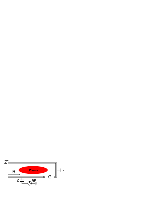
Figure 1: Schematic of the simulation for CCP.

Square cells are used, thus Z direction is uniformly divided to 64 cells and 256 cells are in R. The space and time steps are fixed to all simulations, $\Delta x=0.02/64m$, $\Delta t_{e}=1\times 10^{-10}$s and $\Delta t_{i}=10\Delta t_{e}$. Note here we did not subcycle the MC process to avoid violation the condition of the null collision method for ions. We adopted somewhat a little larger time step to save time, which would result somewhat lower density by a factor of about $0.6\sim 0.8$, but most the physics, such as the sheath thickness, is still preserved. The initial density is uniform of $5\times 10^{15}m^{-3}$ for all cells and 200 particles are placed randomly within one cell. During the simulations, totally about $5-7\times 10^{6}$ particles are traced. One simulation will take about 40 to 60 hours for 1000 rf periods before convergence, in 4 nodes of our cluster. All results are given by averaging over one rf period after reaching equilibrium.

The numerical schemes are also chosen similar to the benchmark problems, except that the electrons are subcycled. The self-bias dc voltages are calculated self consistently from PIC/MC model with Vahedi [32] model. For comparison, fluid model simulations, which have be detailed discussed in our former paper[33], are performed with identical physics parameters, except that the voltage waveforms from the PIC/MC model are used. A typical fluid simulation will take only about 18 hours on a single Intel E2160 CPU, or about $1/20\sim 1/30$ computation cost of implicit PIC/MC simulations.

3 Simulation results

3.1 Self-bias dc voltage

The calculated voltages on the rf powered electrode are plotted in Fig.2, it is very clear that the voltages are in $V=V_{0}\sin\omega_{rf}t+V_{dc}$ form, where $V_{0}$ is 188V, 191V and 195V, $V_{dc}$ is -49V, -74V and -117V for G1, G2 and G4 case, respectively. Due to the potential drop on the capacitor, $V_{0}$ is slightly smaller than $V_{rf}$, and $V_{dc}$ increases with decreasing rf electrode radius. No higher harmonic oscillations are observed in our simulations.

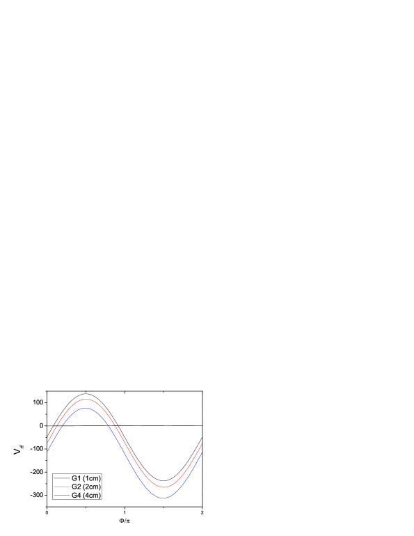
Figure 2: Voltage waveforms on the rf powered electrode.

For clarity, cross-sectional profiles of $\Phi$ at $R=2cm$ for different gap lengths are shown in Fig.3. The potential drop near the rf electrode $V_{a}$ and the potential drop near the grounded electrode $V_{b}$, can be readily read from the figure. Here we have the electrode surface area ratio $A_{b}/A_{a}=1.3$, $1.8$ and $4$, for the G1,G2 and G4 case, respectively. The $V_{a}/V_{b}$ and $A_{b}/A_{a}$ has the relation

$$\frac{V_{a}}{V_{b}}=(\frac{A_{b}}{A_{a}})^{q}.$$ (1)

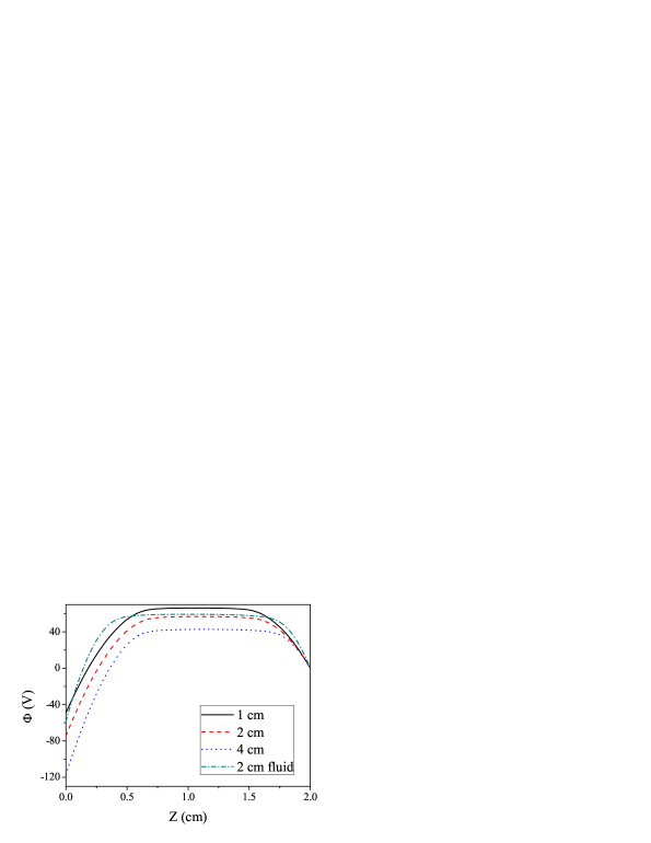
Figure 3: Axial cross-sectional profiles for $\Phi$ at $R=2cm$ for different gap lengths from PIC/MC model. We also plotted the result from fluid model with the gap length of $2cm$ for comparison.

We plotted $V_{a}$, $V_{b}$ and $q$ as function of gap lengths in Fig.4. It can be concluded that $V_{a}$ increases and $V_{b}$ decreases with increasing ${A_{b}}/{A_{a}}$. The $V_{a}$ from the fluid model is smaller than that from PIC/MC model, while the $V_{b}$ is larger, even the fluid model simulation adopted voltage from PIC/MC results. The $q$ is also smaller from fluid model.

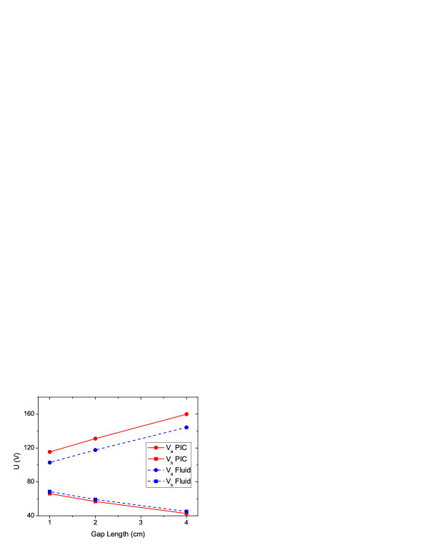
Figure 4: (a)Average potential drop near the rf electrode $V_{a}$ and potential drop near the grounded electrode $V_{b}$; and (b) $V_{a}/V_{b}$ and power $q$ as a function of ${A_{b}}/{A_{a}}$. The solid line is from PIC/MC model and the dashed line is from fluid model

The key issue to understand the problem is the electron and ion mean free length, $\lambda_{e}\approx 3cm$ and $\lambda_{i}\approx 0.03cm$. For $G=1cm$ case (${A_{b}}/{A_{a}}=1.31$), the $q=2.08$, very close to the collisional case where $q=2.21$ [24]. In this case, the gap is narrow, the side wall sheath is thin thus has little effects on the bulk plasmas, the 1D spherical shell model will give a good estimation for $q$. For $G=2cm$ case (${A_{b}}/{A_{a}}=1.77$), the $q=1.45$, same to value $q=1.45$ given by Lieberman’s finite radius model[25]. In this case, the gap length is moderate,as well as the side wall sheath length. For $G=4cm$ case (${A_{b}}/{A_{a}}=4$), the electrode radius is comparable to the electron mean free length, local effect will be significant and the plasma is heavily disturbed by the side sheath, $q$ is can not be predicted by the analytical model, we have $q=0.95$. We can conclude that finite radius effects are always tend to decrease $q$.

The period average potential and field $\Phi$, $E_{z}$ and $E_{r}$ from PIC/MC model are depicted in Fig.5, corresponding results from fluid model are shown in Fig.6, both for G2 case. all for G2 case. Unlike the 1-D symmetric simulation, the potential $\Phi$ is more negative since there are self-bias voltages. The $E_{z}$ in the axial direction has a structure similar to the 1-D simulation, except the drop near the side wall. The $E_{r}$ is small, except near the side wall. Due to the ion sheath near the wall, the $E_{r}$ is very large and positive there, except that $E_{r}$ is negative near the gap since the self-bias voltage is negative. Fluid model gives very similar results. But the fluid results have larger plateau in the center. And the $E_{z}$ given by PIC/MC model is slightly smaller than $E_{z}$ given by fluid model.

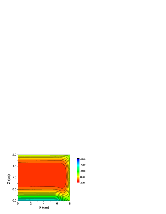
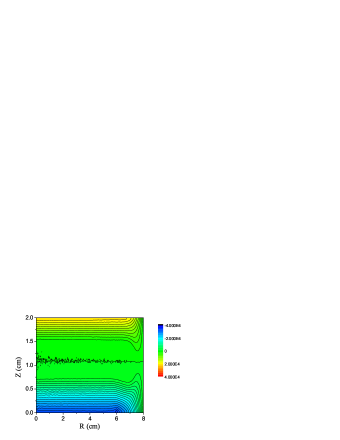
Figure 5: 2D average (a)$\Phi$(V), (b)$E_{z}$ (V/m) and (c)$E_{r}$ (V/m) profiles from PIC/MC model. The gap length is $2cm$.

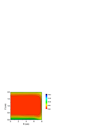
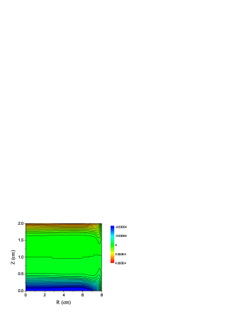
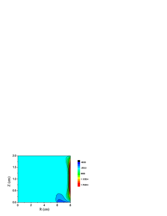
Figure 6: 2D average (a)$\Phi$(V), (b)$E_{z}$ (V/m) and (c)$E_{r}$ (V/m) profiles from fluid model. The gap length is $2cm$.

3.2 Plasma density

The electron densities from PIC/MC model are shown in Fig.7, corresponding results from fluid model are shown in Fig.8, all for different gap length. It can be clearly seen that both fluid model and PIC/MC model give similar results for the peak plasma density and the profiles. The axial cross sections of the density are very similar to the 1D results, except near the gap.

In fluid results, the density profiles are much more flat and smooth, there are only one peak near the gap, for all three cases. This phenomena comes from the well-known numerical diffusion effect. In Eulerian simulations, the discrete equations always give larger diffusive coefficients than the original differential equations in general, even if Flux-Corrected Transport (FCT) method is often used. As a result, fluid model tends to smooth out all the short wave length oscillation and lessens the density gradients.

In PIC/MC results, since the kinetics effects are included, the cases are much more complex. For G1 case, there are only one peak near the gap, the radial density is nearly constant between the gap and the axis, like many other fluid simulations have predicted [29, 30]. For G2 case, the only difference is the self bias voltage, compared to the benchmark problem in our first paper. There are two peaks, the lower one is near the gap, the higher is in the axis, also similar to the benchmark problems. But in this case, self bias dc voltage makes the density gradients between the gap and the axis become smaller. The G4 case has the largest peak density, and there are three peaks, the most high peak is near the gap, the lower peak is near the axis, and the lowest is between the gap and the side wall. As we have discussed, in this case the electron free length is comparable to the electrode radius, electron can be bounced by the radial sheath to gain energy (then increase the densities). On the other hand, when it runs towards the axis, it can decrease the velocity due to the collision. For the change of the velocity, it can be accumulated near the axis then two peaks appears. When the electrons and the ions drift out of the rf powered electrode, they can be trapped and heated in the side wall sheath, and thus form the third peak. These peaks, are inherently kinetic effect, and all are smoothed out in the fluid simulation, even if fluid model can give reasonable density. It also should be noted that the maximum density is G4 case, and the the minimum density is G2 case for PIC/MC model. But the maximum density is G2 case, and the the minimum density is G4 case for fluid model.

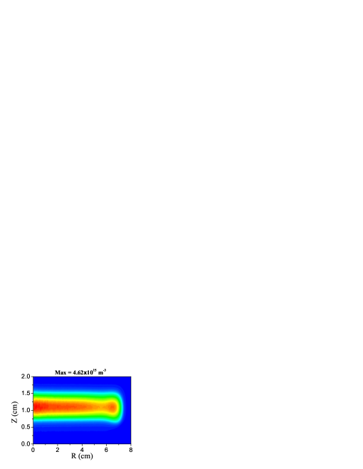
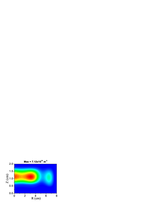
Figure 7: Average electron density profiles from PIC/MC model. The gap lengths are (a)$1cm$, (b)$2cm$ and (c)$4cm$.

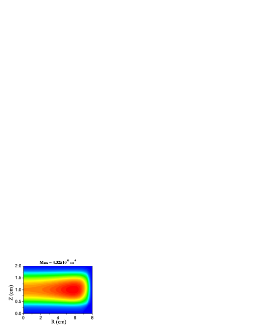
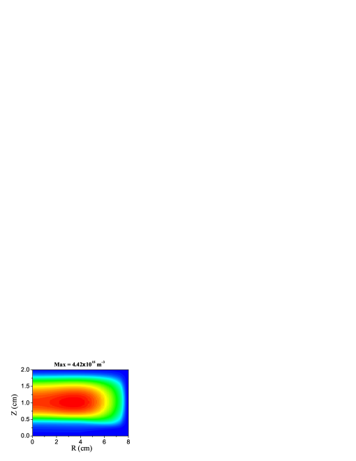
Figure 8: Average electron density profiles from fluid model. The gap lengths are (a)$1cm$, (b)$2cm$ and (c)$4cm$.

For clarity, we plotted the axial and radial cross-sectional profiles for the electron and ion density for different gap lengths Fig.9. For axial profile, PIC/MC model give steeper results, as well as the sheath thickness, again, the reason is the numerical diffusion in the fluid model. Due to the dc bias voltage, the peak is more close to the grounded electrode, but the profile is still close to the 1D results. Note here because we have adopted large time steps in PIC/MC simulations, we have underestimate the max density by a factor of about $0.6\sim 0.8$.

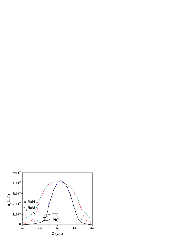
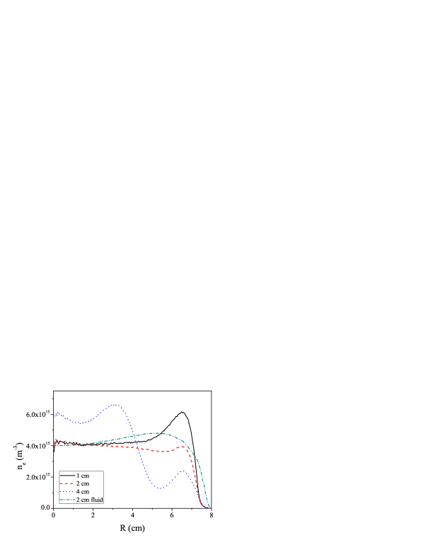
Figure 9: (a) Axial cross-sectional profile at $R=2cm$ of electron and ion density and for $G=2cm$; (b) radial cross-sectional profile of electron density at $Z=1cm$ for different gap lengths, both from PIC/MC model. We also plotted the same results from fluid model with $G=2cm$ for comparison

For radial profile, all three cases give similar side sheath thickness, larger than that from the fluid model. The reason is the same. G4 case gives the largest density. As we have discussed, enhanced heating due to the finite radial length, is responsible for the result. G2 case has similar density to the G1 case and the fluid results in the axis, but gives smaller value at larger radius. It seems that, in this case, finite radial length effect tend to decrease the density, by increasing the side wall ion loss. It should be noted that the peaks near the wall all appeared at the same radial position.

3.3 Electron temperature

We depicted the 2D average electron temperature profiles from PIC/MC model and fluid model in Fig.10, for gap length of $2cm$. The differences are significant. For fluid model, the density are about $4eV$ and nearly constant over very large area. But for PIC/MC model, the profile is saddle like in axial direction. This implies the electron heating mostly occurs in the sheath. Note there is also a peak in the side wall sheath, implying electron heated there, by the oscillating side wall sheath and the $E_{r}$. The most significant difference is near the gap corner, fluid model predict a electron temperature enhancement there, while PIC/MC model give zero temperature because there is a small zone without electrons in all time. Again, this is a result of numerical diffusion effect of fluid model.

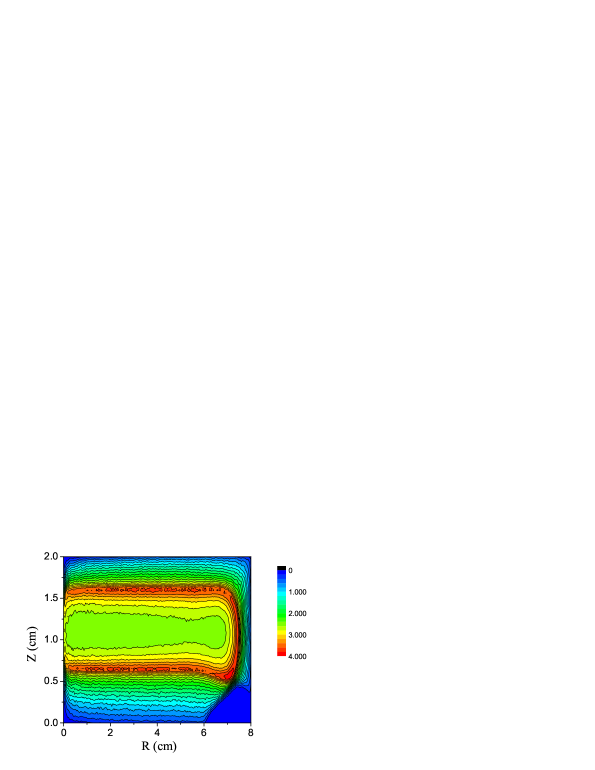
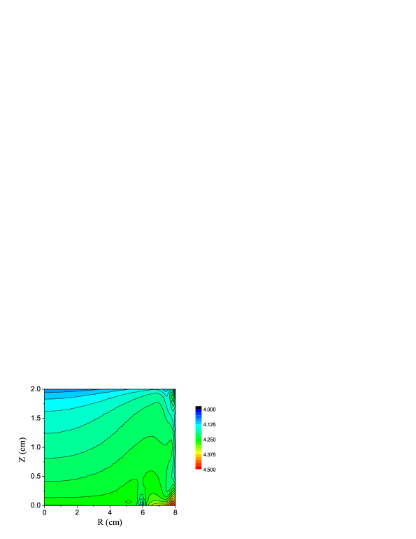
Figure 10: 2D average electron temperature profiles from PIC/MC model(a) and fluid model (b). The gap length is all $2cm$.

For clarity we also plotted the axial cross-sectional profiles at $R=2cm$ of electron temperature for different gap lengths. Again, the profiles are very similar to 1D results, a saddle like form. The temperature given by the fluid model is nearly constant and larger than those given by PIC/MC model. At larger self dc voltage, the peak will tend to move towards the grounded electrode.

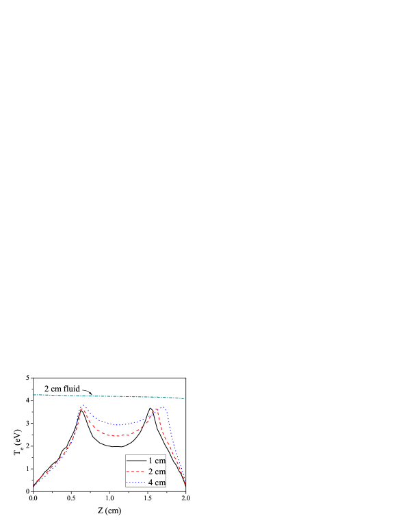
Figure 11: Axial cross-sectional profiles at $R=2cm$ of electron temperature for different gap lengths, both from PIC/MC model. We also plotted the same results from fluid model with $G=2cm$ for comparison

3.4 Ion flux and energy distributions

Fig.12(a) shows the radial distribution of ion flux onto the rf powered electrode for three gap lengths. As can be seen, although G4 case gives the largest flux, the flux is not very uniform, while for the G1 and G2 case, the flux is uniform over the rf powered electrode. It should be noted that the ion flux is larger for G2 case, although the density is smaller. It seems the larger side wall sheath tend to increase the flux to the electrode.

Fig.12(b) shows the ion energy distribution functions (IEDFs) on the rf powered electrode. Due to the pressure is high, the two peaks in the IEDFs are not very clear; and larger gaps give larger average ion energy, because the self bias dc voltage is larger, as we have discussed.

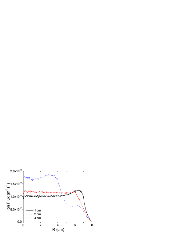
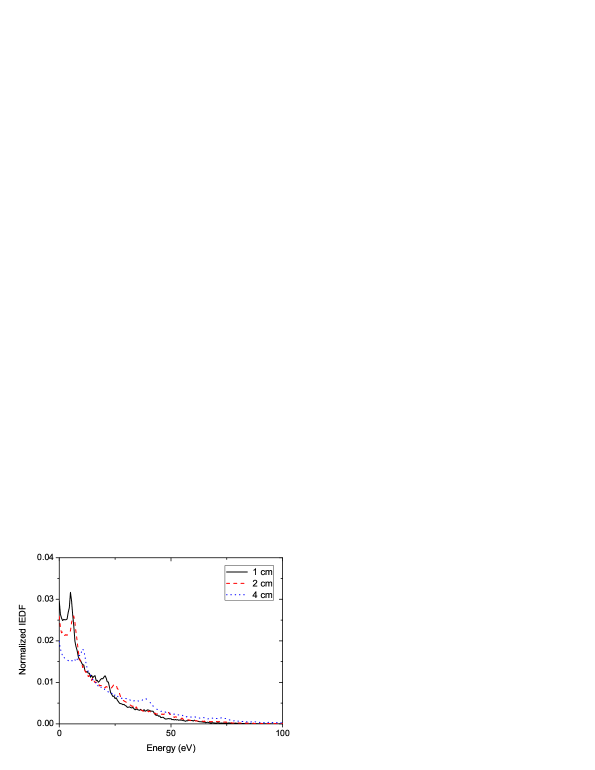
Figure 12: (a)Radial distribution of ion flux onto the rf powered electrode; and (b) ion energy distribution functions on the rf powered electrode, both from PIC/MC model.

4 Discussions and summary

In this paper, we have studied the self-bias dc voltage with 2D PIC/MC model. At small gap length, the dc voltage can be well estimated by 1D spherical shell model[24]; at moderate gap length, the dc voltage can be well estimated from the infinite radius model[25]. However, at small gap length, the dc voltage can not be estimated by the analytic mode, due to electron nonlocal behavior will dominate.

Due to the numerical diffusion effect, although it can give reasonable density values and profiles, fluid model tends to smooth out all the short wave length oscillation and lessen the density gradients. The density and electron temperature profiles given by the PIC/MC model are more steep. Due to nonlocal and kinetic effects, there are several peaks in the density profiles. The simulations validate both PIC/MC model we have adopted and the fluid model.

However, PIC/MC model still has many shortcomings compare to fluid model, which may severely constrain the applications of this model. For example, PIC/MC model is computationally expensive, and is very hard or even practically impossible to couple with chemical reaction model and neutral gas model[34]. Nevertheless, through PIC/MC model, exactly plasma behavior can be predicted, kinetics effects can be preserved. We are trying to give more insights into the physics of CCP with this model.

References

References

- [1] Lieberman M A and Lichtenberg A J 2005 Principles of Plasma Discharges and Materials Processing 2nd edn (New York: Wiley)
- [2] Makabe T and Petrovic Z L 2006 Plasma Electronics: Applications in Microelectronic Device Fabrication (New York: Taylor and Francis Group)
- [3] Kushner M J 2009 J. Phys. D: Appl. Phys. 42 194013
- [4] Kim H C, Iza F, Yang S S, Radmilovic-Radjenovic M, and Lee J K 2005 J. Phys. D: Appl. Phys. 38 R283-R301
- [5] Dijk J, Kroesen G M W and Bogaerts A 2009 J. Phys. D: Appl. Phys. 42 190301
- [6] Georgieva V , Bogaerts A and Gijbels R 2003 J. Appl. Phys. 93 2369
- [7] Boyle P C , Ellingboe A R and Turner M M 2004 Plasma Sources Sci. Technol. 13 493
- [8] Kim H C and Lee J K, 2004 Phys. Rev. Lett. 93, 085003
- [9] Kawamura E, Lieberman M A and Lichtenberg A J 2006 Phys. Plasmas 13 053506
- [10] Bronold F X, Matyash K, Tskhakaya D, Schneider R and Fehske H 2007 J. Phys. D: Appl. Phys. 40 6583
- [11] Donko Z, Schulze J, Heil B G and Czarnetzki U 2009 J. Phys. D: Appl. Phys. 42 025205
- [12] Jiang W, Wang H Y, Zhao S X and Wang Y N 2009 J. Phys. D: Appl. Phys. 42 102005
- [13] Vahedi V, Birdsall C K Lieberman M A DiPeso G and Rognlien T D 1993 Phys. Fluids B 5 2719
- [14] Kawamura E, Lieberman M A and Lichtenberg A J 2008 Plasma Sources Sci. Technol. 17 045002
- [15] Wakayama G and Nanbu K 2003 IEEE Trans. Plasma Sci. 31 638
- [16] Wang H Y, Jiang W and Wang Y N 2009 Comput. Phys. Commun 180 1305-1314
- [17] Lee S H, You S J, Chang H Y and Lee J K 2007 J. Vac. Sci. Technol. A 25 455
- [18] Kim D H and Ryu C M 2007 J. Phys. D: Appl. Phys 41 015207
- [19] Leray G, Chabert P, Lichtenberg A J and Lieberman M A 2009 J. Phys. D: Appl. Phys 42 194020
- [20] Chabert P, Raimbault J L, Levif P, Rax J M and Lieberman M A 2005 Phys. Rev. Lett. 95, 205001
- [21] Lee I, Graves D B and Lieberman M A 2008 Plasma Sources Sci.Technol. 17 015018
- [22] Yonemura S and Nanbu K 2006 Thin Solid Films 506 517
- [23] Bultinck E, Kolev I, Bogaerts A and Depla D 2008 J. Appl. Phys. 103 013309
- [24] Lieberman M A 1989 J. Appl. Phys. 65 4186
- [25] Lieberman M A and Savas S E 1990 J. Vac. Sci. Technol. A 8 1632
- [26] Kawamura E, Vahedi V, Lieberman M A and C K Birdsall 1999 Plasma Sources Sci. Technol. 8 R45
- [27] Smith H B, Charles C, Boswell R W and Kuwahara H 1997 J. Appl. Phys. 82 561
- [28] Yonemura S, Nanbu K and Iwata N 2004 J. Appl. Phys. 96 127
- [29] Rauf S and Kushner M J 1997 J. Appl. Phys. 83 5087
- [30] Rauf S and Kushner M J 1999 IEEE Trans. Plasma Sci. 27 1329
- [31] Kaganovich I D 2002 Phys. Rev. Lett. 89, 265006
- [32] Vahedi V and DiPeso G 1997 J. Comput. Phys.131 149
- [33] Bi Z H, Dai Z L, Xu X, Li Z C and Wang Y N 2009 Phys. Plasmas 16 043510
- [34] Takekida H and Nanbu K 2006 IEEE Trans. Plasma Sci. 34 973