Blume-Capel model on directed and undirected Small-World Voronoi-Delaunay random lattices

Abstract

The critical properties of the spin-$1$ two-dimensional Blume-Capel model on directed and undirected random lattices with quenched connectivity disorder is studied through Monte Carlo simulations. The critical temperature, as well as the critical point exponents are obtained. For the undirected case this random system belongs to the same universality class as the regular two-dimensional model. However, for the directed random lattice one has a second-order phase transition for $q<q_{c}$ and a first-order phase transition for $q>q_{c}$, where $q_{c}$ is the critical rewiring probability. The critical exponents for $q<q_{c}$ was calculated and they do not belong to the same universality class as the regular two-dimensional ferromagnetic model.

I Introduction

There has been recently an increasing interest in the study of networks which are not usual regular lattices. This growing interest, principally among physicists, comes mainly from the fact that they can model complex systems in real world networks bara . In special, small-world (SW) networks ws have been much studied as they furnish a simple way to attempt to describe complex topologies such as social and economic organizations, the speed of disease spread, connectivities of computers, just to cite a few of them bara .

As is usual, a rigorous treatment to get the properties of a real physical realization on such complex systems is a quite difficult task. However, one expects that simple theoretical models, such as the discrete spin Ising model, could be able to capture the main features of the actual complicated processes occurring on real networks. In this direction, the spin-$1/2$ Ising model has been studied on SW networks and, for exchange interactions which are independent of the length distance of the spins, one gets a second-order phase transition at a finite critical temperature $T_{c}$ barrat ; novo ; hinc .

Sánches et al. san introduced the asymmetric directed SW networks and for an Ising like spin system they showed that a first-order phase transition takes place when the rewiring probability $q$ is greater than a critical value $q_{c}$. The same result has been achieved by Lima et al. when treating the spin-$1,~{}3/2$ and $2$ Ising model on the same networks lima .

In most of the above theoretical models the undirected, as well as the directed SW networks, have been constructed by taking, as an initial step, a regular pure hypercubic lattice san . It will be very interesting, thus, to see what should be the behavior of SW networks built up over an already random system, such as the Voronoi-Delaunay random lattices. So, in this paper, we study the spin-$1$ Blume-Capel model on undirected and directed SW networks constructed from an initial Voronoi-Delaunay random lattice. The purpose here is indeed two-fold: first, we would like to see the effect of the disorder itself on the spin-$1$ model on this undirected lattice (since, for the spin-$3/2$ model wel there has been a change in its universality class) and, secondly, the behavior of spin models on SW networks obtained from random number of nearest neighbors. In the next section we present the SW networks, the model and the simulation background. The results and discussions are presented in the last section.

II SW networks, Model and Simulation

Undirected Voronoi-Delaunay random lattice - The Voronoi construction, or tessellation, for a given set of points in the plane can be defined as follows christ . Initially, for each point one determines the polygonal cell consisting of the region of space nearer to that point than any other point. Then one considers that the two cells are neighboring when they possess an extremity in common. From the Voronoi tessellation the dual lattice can be obtained by the following procedure: $(i)$ when two cells are neighbors, a link is placed between the two points located in the cells; $(ii)$ from the links one obtains the triangulation of space that is called the Delaunay lattice; $(iii)$ the Delaunay lattice is dual to the Voronoi tessellation in the sense that points corresponding to cells link to edges, and triangles to the vertices of the Voronoi tessellation.

Directed Voronoi-Delaunay SW network - We use here the same process defined by Sánchez et al. san for directing the Voronoi-Delaunay random lattice. In this case, we start with the Voronoi construction, or tessellation, as described in the previous paragraph, by creating the random two-dimensional lattice consisting of sites linked to their nearest neighbors by both outgoing and incoming links. Then, with probability $q$, we reconnect nearest-neighbor outgoing links to a different site chosen at random. After repeating this process for every link, we are left with a network with a density $q$ of random two-dimensional lattice directed links. Therefore, with this procedure every site will have exactly the same amount of undirected random two-dimensional lattice outgoing links and a varying (random) number of incoming links.

Model - We consider now the two-dimensional spin-$1$ Blume-Capel model on these Poissonian random lattices. The Blume-Capel Model is a generalization of the standard Ising model kobe and was originally proposed for spin-$1$ to account for first-order phase transition in magnetic systems BC ; BC2 . The Hamiltonian can be written as

$$H=-J\sum_{<i,j>}S_{i}S_{j}+\Delta\sum_{i}S_{i}^{2},$$ (1)

where the first sum runs over all nearest-neighbor pairs of sites (points in the Voronoi construction) and the spin-$1$ variables $S_{i}$ assume values $\pm 1,0$. In eq. (1) $J$ is the exchange coupling and $\Delta$ is the single ion anisotropy parameter. The second sum is taken over the $N$ spins on a $D$-dimensional lattice. The case where $S=1$ has been extensively studied by several approximate techniques in two- and three-dimensions and its phase diagram is well established BC ; BC2 ; BC3 ; BC4 ; BC5 ; BC6 ; BC7 . The case $S>1$ has also been investigated according to several procedures BC8 ; BC9 ; BC10 ; BC11 ; BC12 ; BC13 ; landaupla .

Simulations - The simulations have been performed for $\Delta=0$, which is the simplest case and where we have some results in the literature to compare with. The lattices comprised different sizes with $N$ ranging from $N=250,500,1000,2000,4000,8000$, and $16000$, where $N$ is total umber of sites. For simplicity, the linear length of the system is defined here in terms of the size of a regular two-dimensional lattice $L=N^{1/2}$. For each system size quenched averages over the connectivity disorder are approximated by averaging over $R=100$ ($N=500$ to $4000$), $R=50$ ($N=8000$) and $R=25$ ($N=16000$) independent realizations. For each simulation we have started with a uniform configuration of spins (the results are, however, independent of the initial configuration). We ran $2.52\times 10^{6}$ Monte Carlo steps (MCS) per spin with $1.2\times 10^{5}$ configurations discarded for thermalization using the “perfect” random-number generator nu . In both cases we have employed the heat bath algorithm and for every $12$th MCS, the energy per spin, $e=E/N$, and magnetization per spin, $m=\sum_{i}S_{i}/N$, were measure and recorded in a time series file. From these thermodynamic quantities the behavior of the transition can be analyzed.

From the series of the energy measurements we can compute, by re-weighting over a controllable temperature interval $\Delta T$, the average energy, the specific heat, and the energy fourth-order cumulant which are respectively given by

$$u(K)=[<E>]_{av}/N,$$ (2)

$$C(K)=K^{2}N[<e^{2}>-<e>^{2}]_{av},$$ (3)

$$B(K)=[1-\frac{<e^{4}>}{3<e^{2}>^{2}}]_{av},$$ (4)

where $K=J/k_{B}T$, with a normalized exchange $J=1$, and $k_{B}$ is the Boltzmann constant. In the above equations $<...>$ stands for thermodynamic averages and $[...]_{av}$ for averages over the different realizations. Similarly, we can derive from the magnetization measurements the average magnetization, the susceptibility, and the magnetic cumulants,

$$m(K)=[<|m|>]_{av},$$ (5)

$$\chi(K)=KN[<m^{2}>-<|m|>^{2}]_{av},$$ (6)

$$U_{2}(K)=[1-\frac{<m^{2}>}{3<|m|>^{2}}]_{av},$$ (7)

$$U_{4}(K)=[1-\frac{<m^{4}>}{3<|m|>^{2}}]_{av}.$$ (8)

Further useful quantities involving both the energy and magnetization are their derivatives

$$\frac{d[<|m|>]_{av}}{dK}=[<|m|E>-<|m|><E>]_{av},$$ (9)

$$\frac{d\ln[<|m|>]_{av}}{dK}=[\frac{<|m|E>}{<|m|>}-<E>]_{av},$$ (10)

$$\frac{d\ln[<|m^{2}|>]_{av}}{dK}=[\frac{<|m^{2}|E>}{<|m^{2}|>}-<E>]_{av}.$$ (11)

In order to get the transition temperature, as well as to determine the order of the transition of this model, we apply the finite-size scaling (FSS) procedure. Initially, we search for the minima of the energy fourth-order cumulant given by Eq. (4). This quantity gives a qualitative, as well as a quantitative, description of the order of the transition mdk . For instance, it is known janke0 that this parameter takes a minimum value $B_{min}$ at the effective transition temperature $T_{c}(N)$. One can also show kb that for a second-order transition, $\lim_{N\to\infty}$ $(2/3-B_{min})\rightarrow 0$, even at $T_{c}$, while at a first-order transition the same limit measuring the same quantity is small and $(2/3-B_{min})\neq 0$.

A more quantitative analysis can be carried out through the FSS of the energy fluctuation $C_{max}$, the susceptibility maxima $\chi_{max}$, and the minima of the Binder cumulants $B$, $U_{2}$ and $U_{4}$.

If the hypothesis of a first-order phase transition is correct, we should then expect, for large systems sizes, an asymptotic FSS behavior of the form wj ; pbc ,

$$C_{max}=a_{C}+b_{C}N+...$$ (12)

$$\chi_{max}=a_{\chi}+b_{\chi}N+...$$ (13)

$$B_{min}=a_{B_{i}}+b_{B_{i}}/N+...$$ (14)

On the other hand, if the hypothesis of a second-order phase transition is correct, we should then expect, for large systems sizes, an asymptotic FSS behavior of the form

$$C=C_{reg}+L^{-\alpha/\nu}f_{C}(x)[1+...],$$ (15)

$$[<|m|>]_{av}=L^{-\beta/\nu}f_{m}(x)[1+...],$$ (16)

$$\chi=L^{-\gamma/\nu}f_{\chi}(x)[1+...],$$ (17)

$$\frac{d\ln[<|m|^{p}>]_{av}}{dK}=L^{1/\nu}f_{p}(x)[1+...],$$ (18)

where $C_{reg}$ is a regular background term, $\nu$, $\alpha$, $\beta$, and $\gamma$ are the usual critical exponents, and $f_{i}(x)$ are FSS functions with $x=(K-K_{c})L^{1/\nu}$ being the scaling variable, and the brackets $[1+...]$ indicate corrections-to-scaling terms.

In all cases, we estimated the error bars from the fluctuations among the different realizations. Note that these errors contain both, the average thermodynamic error for a given realization and the theoretical variance for infinitely accurate thermodynamic averages which are caused by the variation of the quenched, random geometry of the lattices.

III Results and discussion

III.1 undirected random two-dimensional lattice

By applying standard re-weighting techniques to each of the $R$ time-series data we first determined the temperature dependence of $C_{i}(K)$, $\chi_{i}(K)$,…, $i=1$,…,$R$, in the neighborhood of the simulation point $K_{0}$. Once the temperature dependence is known for each realization, we can easily compute the disorder average, e.g., $C(K)=\sum^{R}_{i=1}C_{i}(K)/R$, and then determine the maxima of the averaged quantities, e.g., $C_{max}(K_{max})=max_{K}C(K)$. The variable $R$ represents the number of replicas in our simulations.

In order to estimate the critical temperature we calculate the second and fourth-order Binder cumulants given by eqs. (7) and (8), respectively. It is well known that these quantities are independent of the system size and should intercept at the critical temperature binder . In Fig. 1 the fourth-order Binder cumulant is shown as a function of the $K$ for several values of $N$. Taking the largest lattices we have $K_{c}=0.3560(5)$. To estimate $U^{*}_{4}$ we note that it varies little at $K_{c}$ so we have $U^{*}_{4}=0.6058(6)$. From the second-order cumulant (not shown) we similarly get $K_{c}=0.3561(4)$ and $U^{*}_{2}=0.6416(3)$. One can see that the agreement of the critical temperature is quite good and $U^{*}_{4}$ is definitely close to the universal value $U^{*}_{4}\sim 0.61$ for the same model on the regular $2D$ lattice.

Figure 1: Fourth-order Binder cumulant as a function of $K$ for several values of the system size $N=500,1000,2000,4000,8000$ and $16000$.

The correlation length exponent can be estimated from the derivatives given by eq. (18). Figure 2 shows the maxima of the logarithm derivatives as a function of the logarithm of the lattice size $L$ for $p=1$ and $p=2$. From the linear fitting one gets $\nu=0.984(6)$ ($p=1$) and $\nu=0.983(5)$ ( $p=2$), which is again next to the regular lattice exponent $\nu=1$.

Figure 2: Log-log plot of the maxima of the logarithmic derivative $\frac{d\ln[<|m|^{p}>]}{dK}$ versus the lattice size $L=N^{1/2}$ for $p=1$ (circle) and $p=2$ (square). The solid lines are the best linear fits.

In order to go further in our analysis we also computed the modulus of the magnetization at the inflection point and the maximum of the magnetic susceptibility. The logarithm of these quantities as a function of the logarithm of $L$ are presented in Figures 3 and 4, respectively. A linear fit of these data gives $\beta/\nu=0.135(9)$ from the magnetization and $\gamma/\nu=1.751(4)$ from the susceptibility which should be compared to $\beta/\nu=0.125$ and $\gamma/\nu=1.75$ obtained for a regular $2D$ lattice. One can see that for this undirected random lattice we get the same universal critical behavior as the regular lattice model, in the same way as has been reported for the diluted spin-$1/2$ Ising model paulo .

Figure 3: Plot of the logarithm of the modulus of the magnetization at the inflection point as a function of the logarithm of $L=N^{1/2}$. The solid line is the best linear fit.

Figure 4: Log-log plot of the susceptibility maxima $\chi_{max}$ as a function of the logarithm of $L=N^{1/2}$. The solid line is the best linear fit.

III.2 directed random two-dimensional lattice

In Fig. 5 we show the dependence of the magnetization as a function of the temperature, obtained from simulations on directed random two-dimensional lattice, with $N=16000$ sites, and two values of probability $q$, namely $q=0.1$ for second-order phase transition and $q=0.9$ for first-order phase transition, respectively.

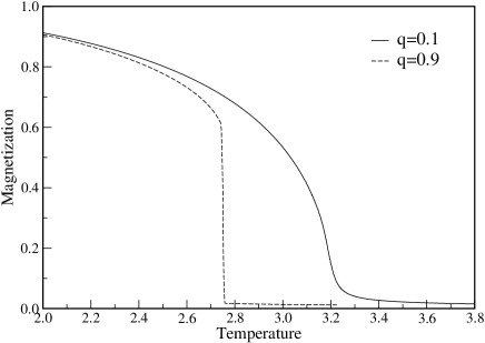
Figure 5: Magnetization as a function of the temperature, for $N=16000$ sites. It is clear a second-order phase transition for $q=0.1$, and a first-order phase transition for $q=0.9$, respectively.

The energetic Binder cumulant as a function of the reduced temperature $K$ for $q=0.1$, and different lattice sizes, is displayed in the Figure 6, where a characteristic second-order phase transition is observed.

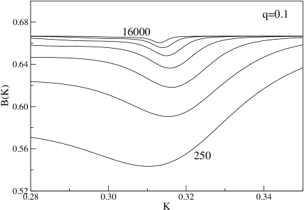
Figure 6: Energetic Binder cumulant as a function of the reduced temperature $K$ for $q=0.1$ and lattice sizes $N=250,500,1000,2000,4000,8000$, and $16000$ from bottom to top.

On the other hand, in the Figure 7 we display the same plot as in Figure 6, but now for $q=0.4$, where we can see that a first-order transition is present for this value of the rewiring probability.

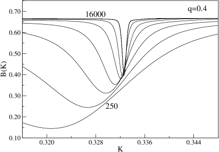
Figure 7: The same display the Fig. 6, but now for $q=0.4$ and size $N=250,500,1000,2000,4000,8000$, and $16000$ from bottom to top.

In Fig.8, the difference $2/3-B_{min}$ is shown as a function of the parameter $1/N$ for different probabilities $q$. For values $q<q_{c}\approx 0.35$, a second-order transition takes place since in the $\lim_{N\to\infty}$ $(2/3-B_{i,min})=0$, even at $T_{c}$. However, for $q>q_{c}$ a first-order transition is observed, because one has $(2/3-B_{i,min})\neq 0$. For instance, for $q=0.4$ we get $(2/3-B_{min})=0.273(3)$.

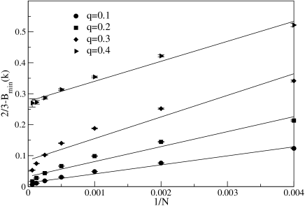
Figure 8: Plot of $2/3-B_{min}$ at $T_{c}$ as a function of logarithm of $1/N$ for several values of the system size $N=250,500,1000,2000,4000,8000$ and $16000$, and $q=0.1,0.2$, $0.3$, and $0.4$.

In Fig. 9 the fourth-order Binder cumulant is shown as a function of the $K$ for several values of $N$ and $q=0.1$. Taking the largest lattices we have $K_{c}=0.3109(6)$. To estimate $U^{*}_{4}$ we note that it varies little at $K_{c}$ so we have $U^{*}_{4}=0.326(4)$. From the second-order cumulant (not shown) we similarly get $K_{c}=0.31078(3)$ and $U^{*}_{2}=0.538(2)$. For other values of $q$ we have: for $q=0.2$, $K_{c}=0.3114(6)$ and $U^{*}_{4}=0.326(5)$ and $K_{c}=0.31164(5)$ and $U^{*}_{2}=0.534(7)$; for $q=0.3$, $K_{c}=0.32154(8)$ and $U^{*}_{4}=0.327(5)$, and $K_{c}=0.32137(5)$ and $U^{*}_{2}=0.556(4)$. One can see that the agreement of the critical temperature is quite good and $U^{*}_{4}$ is definitely different from the universal value $U^{*}_{4}\sim 0.61$ for the same model on the regular $2D$ lattice and undirected Voronoi-Delaunay random lattice.

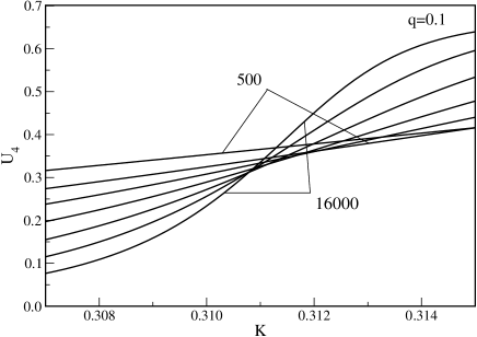
Figure 9: Fourth-order Binder cumulant as a function of $K$ for several values of the system size $N=500,1000,2000,4000,8000$ and $16000$, and $q=0.1$.

Fig. 10 displays the behavior of the magnetization fourth-order cumulant for $q=0.9$ in a narrow range of $K$, where one can note a different behavior leading to a first-order phase transition.

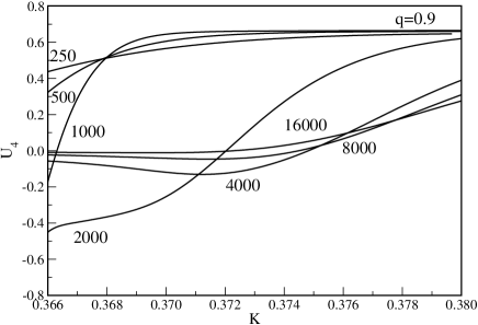
Figure 10: Fourth-order Binder cumulant as a function of $K$ for several values of the system size $N=250,500,1000,2000,4000,8000$ and $16000$, and $q=0.9$.

In our analysis we also computed the modulus of the magnetization at the inflection point, $T=T_{c}$ for $q=0.1,0.2,$ and $0.3$ . The logarithm of these quantities as a function of the logarithm of $L$ are presented in Figure 11. A linear fit of these data gives $\beta/\nu=0.421(7),0.400(5)$ and $0.338(5)$ from the magnetization for $q=0.1,0.2$, and $0.3$, respectively. These results are totally different of $\beta/\nu=0.125$ obtained for a regular $2D$ lattice.

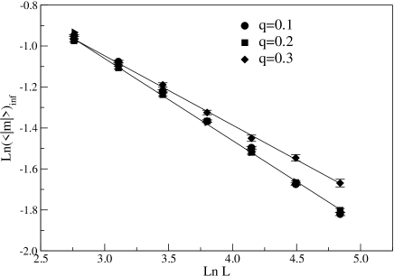
Figure 11: Plot of the logarithm of the modulus of the magnetization at the inflection point as a function of $L=N^{1/2}$ for several values of the system size $N=250,500,1000,2000,4000,8000$ and $16000$, and $q=0.1,0.2,$ and $0.3$.

In Fig. 12 the logarithm plot of the susceptibility at $T_{c}$ as a function of the logarithm of $L=N^{1/2}$ is presented. A linear fit of these data gives, at $T=T_{c}$, $\gamma/\nu=1.101(4),1.138(5)$ and $1.312(7)$. Similarly, from the maximum of the magnetic susceptibility (not shown) one gets $\gamma/\nu=1.130(14),1.156(12)$ and $1.312(3)$ for $q=0.1,0.2$ and $0.3$, respectively, which again is totally different of $\gamma/\nu=1.75$ obtained for a regular $2D$ lattice.

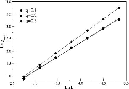
Figure 12: Logarithmic of the susceptibility at $T_{c}$ as a function of the logarithmic of $L=N^{1/2}$ for several values of the system size $N=250,500,1000,2000,4000,8000$ and $16000$, and $q=0.1,0.2,$ and $0.3$.

Finally, in order to calculate the exponents $1/\nu$ , we use the maxima of the logarithmic derivative as defined in Eq. (18). A plot of this quantity versus the lattice size $L=N^{1/2}$ for $p=1$ is shown in Figure 13. From this figure one gets $1/\nu=1.105(8)$, $1.164(11)$ and $1.349(3)$. Similarly, for $p=2$ (not shown) we have $1/\nu=1.107(7),1.167(11)$ and $1.349(3)$ for $q=0.1,0.2$ and $0.3$, respectively, which are also again different from $1/\nu=1$ obtained for a regular $2D$ lattice.

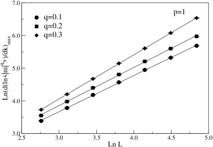
Figure 13: Log-log plot of the maxima of the logarithmic derivative $\frac{d\ln[<|m|^{p}>]}{dK}$ versus the lattice size $L=N^{1/2}$ for $p=1$ and several values of the system size $N=250,500,1000,2000,4000,8000$ and $16000$, and $q=0.1,0.2,$ and $0.3$.

Thus, from the above results, there is a strong indication that the spin-1 Blume-Capel model on a undirected Voronoi lattice is in same universality class as its regular lattice counterpart, in contrast with the spin-$3/2$ model where a change in the exponents has been achieved wel . On the other hand, on a directed SW Voronoi lattice, the exponents here obtained for $q<q_{c}$, where a second order phase transition is obtained in two dimensions, are different from the spin-$1$ Blume-Capel model on regular $2D$ lattices. Therefore, for $q<q_{c}$ not only the exponents, but also the fourth-order cumulants, show a strong indication that this model is not in the same universality class than its regular $2D$ lattice, with varying exponents as a function of $q$. For $q>q_{c}$, we have a first-order phase transition.

We believe that the above behavior should be qualitatively the same for crystal field $\Delta<\Delta_{t}$, where $\Delta_{t}$ is the value where one has a tricritical point in the model on a regular lattice. However, there are still some open questions, for instance: i) the effect of the nearest-neighbor disorder on the undirected lattice for $\Delta>\Delta_{t}$, i.e. in the range of a first-order transition. One can ask whether that will result on a second-order transition with strong violation of universality, as happens in the regular lattice random-bond model studied by Malakis et al. malakis ; ii) the effect of large crystal field on the SW networks where a first-order already takes place on the regular lattice. Work in this direction is now in progress.

References

- (1) R. Albert and A.-L. Barabási, Rev. Mod. Phys. 74, 47 (2002).
- (2) D. J. Watts and S. W. Strogatz, Nature (London) 393, 440 (1998).
- (3) A. Barrat and M. Weigt, Eur. Phys. J. B 13, 547 (2000).
- (4) M. A. Novotny and Shannon M. Wheeler, Braz. J. Phys. 34, 395 (2004).
- (5) M. Hinczewski and A. N. Berker, Phys. Rev. E 73, (2006).
- (6) A. D. Sánches, J. M. López, M. A. Rodrígues, Phys. Rev. Lett. 88, 048701 (2002).
- (7) F. W. S. Lima, E. M. S. Luz, and R. N. Costa Filho, Multidiscipline Modeling in Mat. and Str. 4, 1 (2009).
- (8) F. W. S. Lima and J. A. Plascak, Braz. J. Phys. 36, 660 (2006).
- (9) N. H. Christ, R. Friedberg and T. D. Lee, Nucl. Phys. B 202, 89 (1982); B 210 [FS6] 310, 337 (1982).
- (10) S. Kobe, Braz. J. Phys. 30, 649 (2000).
- (11) M. Blume, Phys. Rev. 141, 517 (1966); H. W. Capel, Physica (Amsterdam) 32, 966 (1966).
- (12) M. Blume, V. J. Emery, and R. B. Griffths, Phys. Rev. A 4, 1071 (1971).
- (13) D. M. Saul, M. Wortis and D. Staufer, Phys. Rev. B 9, 4964 (1974).
- (14) A. K. Jain and D. P. Landau, Phys. Rev. B 22, 445 (1980).
- (15) O. F. de Alcantara Bonfim, Physica A 130, 367 (1985).
- (16) A. N. Berker and M. Wortis, Phys. Rev B 14, 4946 (1976).
- (17) S. Moss de Oliveira, P. M. C. de Oliveira and F. C. Sá Barreto, J. Stat. Phys. 78, 1619 (1995).
- (18) J. A. Plascak, J. G. Moreira and F. C. Sá Barreto, Phys. Lett. A 173, 360 (1993).
- (19) M. N. Tamashiro and S. R. Salinas, Phys. A 211, 124 (1994).
- (20) J. C. xavier, F. C. Alcaraz, D. Peña Lara and J. A. Plascak, Phys. Rev. B 57, 11575 (1998).
- (21) D. Peña lara and J. A. plascak, Int. J. Mod. Phys. B 12, 2045 (1998).
- (22) F. C. Sá barreto and O. F. Alcantara Bonfim, Physica A 172, 378 (1991).
- (23) A. Bakchinch, A. Bassir and A. Benyoussef, Phyica A 195, 188 (1993).
- (24) J. A. Plascak and D. P. Landau, Phys. Rev. E 67, R015103 (2003). (2003)
- (25) P. L’Ecuyer, Commun. ACM 31, 742 (1988).
- (26) M.S.S. Challa, D. P. Landau, K. Binder, Phys. Rev. B, 34, 1841 (1986).
- (27) W. Janke, Phys. Rev. B 47, 14757 (1993).
- (28) K. Binder, D. J. Herrmann, in Monte-Carlo Simulation in Statistical Phys., edited by P. Fulde (Springer-Verlage,Berlin, 1988), p. 61-62.
- (29) W. Janke, R. Villanova, Phys. Lett. A 209, 179 (1995).
- (30) P. E. Berche, C. Chatelain, B. Berche, Phys. Rev. Lett. 80, 297 (1998)
- (31) K. Binder, Z. Phys. B 43, 119 (1981).
- (32) P. H. L. Martins and J. A. Plascak, Phys. Rev. E 76, 012102 (2007).
- (33) A. Malakis et al., Physical Rev. B 79, 011125 (2009).