The tail empirical process for long memory stochastic volatility sequences

Abstract

This paper describes the limiting behaviour of tail empirical processes associated with long memory stochastic volatility models. We show that such a process has dichotomous behaviour, according to an interplay between the Hurst parameter and the tail index. On the other hand, the tail empirical process with random levels never suffers from long memory. This is very desirable from a practical point of view, since such a process may be used to construct the Hill estimator of the tail index. To prove our results we need to establish new results for regularly varying distributions, which may be of independent interest.

1 Introduction

The goal of this article is to study weak convergence results for the tail empirical process associated with some long memory sequences. Besides of theoretical interests on its own, the results are applicable in different statistical procedures based on several extremes. A similar problem was studied in case of independent, identically distributed random variables in [12], or for weakly dependent sequences in [11], [10], [9], [19].

Our set-up is as follows. Assume that $\{X_{i}\,,\ i\in\mathbb{Z}\}$, is a stationary Gaussian process with unit variance and covariance

$$\rho_{i-j}=\mathrm{cov}(X_{i},X_{j})=|i-j|^{2H-2}\ell_{0}(|i-j|)\;,$$ (1)

where $H\in(1/2,1)$ is the Hurst exponent and $\ell_{0}$ is a slowly varying function at infinity, i.e. $\lim_{t\to\infty}\ell_{0}(tx)/\ell_{0}(x)=1$ for all $x>0$. The sequence in this case is referred to as an LRD Gaussian sequence. We also consider weakly dependent Gaussian sequences, i.e. such that $\sum_{j=1}^{\infty}|\mathrm{cov}(X_{1},X_{j+1})|<\infty$.

We shall consider a stochastic volatility process defined as

$$Y_{i}=\sigma(X_{i})Z_{i},\qquad i\in\mathbb{Z},$$

where $\sigma(\cdot)$ is a nonnegative, deterministic function and that $\{Z,Z_{i}$, $i\in\mathbb{Z}\}$, is a sequence of i.i.d. random variables, independent of the process $\{X_{i}\}$. We note, in particular, that if ${\mathbb{E}}[Z^{2}]<\infty$ and ${\mathbb{E}}[Z]=0$, then the $Y_{i}$s are uncorrelated, no matter the assumptions on dependence structure of the underlying Gaussian sequence.

Stochastic volatility models have become popular in financial time series modeling. In particular, if $H\in(1/2,1)$, these models are believed to capture two standardized features of financial data: long memory of squares or absolute values, and conditional heteroscedascity. If $\sigma(x)=\exp(x)$, then the model is referred to in the econometrics literature as Long Memory in Stochastic Volatility (LMSV) and was introduced in [4]. For an overview of stochastic volatility models with long memory we refer to [7].

Let $F=F_{i}$, $i\geq 1$, be the marginal distribution of $Y_{i}$. We want to consider the case where $F$ belongs to the domain of attraction of an extreme value distribution with positive index $\gamma$, i.e. there exist sequences $u_{n}$, $n\geq 1$, $u_{n}\to\infty$, and $\sigma_{n}$, $n\geq 1$, such that the associated conditional tail distribution function

$$T_{n}(x)=\frac{\bar{F}(u_{n}+\sigma_{n}x)}{\bar{F}(u_{n})},\qquad x\geq 0,\;n\geq 1,$$ (2)

satisfies

$$\lim_{n\to\infty}T_{n}(x)=T(x)=\left(1+x\right)^{-1/\gamma}\;,\quad x\geq 0\;.$$ (3)

For the stochastic volatility model, this will be obtained through a further specification. Let $F_{Z}$ be the marginal distribution of the noise sequence. We will assume that for some $\alpha\in(0,\infty)$,

$$\bar{F}_{Z}(z)={\mathbb{P}}(Z>x)=x^{-\alpha}\ell(x)\;,$$ (4)

where $\ell$ is again a slowly varying function. Assuming (4) and ${\mathbb{E}}[\sigma^{\alpha+\epsilon}(X_{1})]<\infty$ for some $\epsilon>0$, we conclude by Breiman’s Lemma [5] (see also [18, Proposition 7.5]) that

$$\bar{F}(x)={\mathbb{P}}(Y_{1}>x)={\mathbb{P}}(\sigma(X_{1})Z_{1}>x)\sim{\mathbb{E}}[\sigma^{\alpha}(X_{1})]{\mathbb{P}}(Z_{1}>x)\;,\ \mbox{ as }x\to\infty.$$

Consequently, $\bar{F}(\cdot)$ satisfies (3) with $\sigma_{n}=u_{n}$ and $\gamma=1/\alpha$.

Similarly to [19], we define the tail empirical distribution function and the tail empirical process, respectively, as

$$\tilde{T}_{n}(s)=\frac{1}{n\bar{F}(u_{n})}\sum_{j=1}^{n}1_{\{Y_{j}>u_{n}+u_{n}s\}}\;,$$

and

$$e_{n}(s)=\tilde{T}_{n}(s)-T_{n}(s)\;,\ s\in[0,\infty)\;.$$ (5)

From [19] we conclude that under appropriate mixing and other conditions on a stationary sequence $Y_{i}$, $i\geq 1$, the tail empirical process converges weakly and the limiting covariance is affected by dependence. In our case, the results [19] do not seem applicable. In fact, it will be shown that we have two different modes of convergence. If $u_{n}$ is large, then $\sqrt{n\bar{F}(u_{n})}$ is the proper scaling factor and the limiting process is Gaussian with the same covariance structure as in case of i.i.d. random variables $Y_{i}$. Otherwise, if $u_{n}$ is small, then the limit is affected by long memory of the Gaussian sequence. The scaling is different and the limit may be non-normal. These results are presented in Section 2.1. Note that a similar dichotomous phenomenon was observed in the context of sums of extreme values associated with long memory moving averages, see [16] for more details. On the other hand, this dichotomous behaviour is in contrast with the convergence of point processes based on stochastic volatility models with regularly varying innovations, where (long range) dependence does not affect the limit (See [6]).

The process $e_{n}(\cdot)$ is unobservable in practice, since the parameter $u_{n}$ depends on the unknown distribution $F$. Also, $u_{n}$ being large or small depends on a delicate balance between the tail index $\alpha$ and the Hurst parameter $H$. In order to overcome this, we consider as in [19] a process with random levels. There, we set $k=n\bar{F}(u_{n})$ and replace the deterministic level $u_{n}$ by $Y_{n-k:n}$, where $Y_{n:n}\geq Y_{n-1:n}\geq\cdots\geq Y_{1:n}$ are the increasing order statistics of the sample $Y_{1},\dots,Y_{n}$. The number $k$ can be thought as the number of extremes used in a construction of the tail empirical process. It turns out that if the number of extremes is small (which corresponds to a large $u_{n}$ above), then the limiting process changes as compared to the one associated with $e_{n}(\cdot)$, but the speed of convergence remains the same. This has been already noticed in [19] in the weakly dependent case. On the other hand, if $k$ is large, then the scaling from $e_{n}(\cdot)$ is no longer correct (see Corollary 2.5). In fact, the process with random levels has a faster rate of convergence and we claim in Theorem 2.6 that the rate of convergence and the limiting process are not affected at all by long memory, provided that a technical second order regular variation condition is fulfilled. The reader is referred to Section 2.2. On the other hand, it should be pointed out that our results are for the long memory stochastic volatility models. It is not clear for us whether such phenomena will be valid for example for subordinated long memory Gaussian sequences with infinite variance.

The results for the tail empirical process $e_{n}(\cdot)$ allow us to obtain asymptotic normality and non-normality of intermediate quantiles, as described in Corollary 2.4. On the other hand, the tail empirical process with random levels allows the study of the Hill estimator of the tail index $\alpha$ (Section 2.3). Consequently, as shown in Corollary 2.7, long memory does not have influence on its asymptotic behaviour. These theoretical observations are justified by simulations in Section 3.

Last but not least, we have some contribution to the theory of regular variation. To establish our results in the random level case, we need to work under a second order regular variation condition. Consequently, one has to establish in a Breiman’s-type lemma that such a condition is transferable from $\bar{F}_{Z}$ to $\bar{F}$. This is done in Section 2.4.

2 Results

2.1 Tail empirical process

Let us define a function $G_{n}$ on $(-\infty,\infty)\times[0,\infty)$ by

$$G_{n}(x,s)=\frac{{\mathbb{P}}(\sigma(x)Z_{1}>(1+s)u_{n})}{{\mathbb{P}}(Z_{1}>u_{n})}\;.$$ (6)

By Breiman’s Lemma and the regular variation of $\bar{F}_{Z}$, we conclude that for each $s\in[0,1]$, this function converges pointwise to $T(s)G(x)$, where $G(x)=\sigma^{\alpha}(x)$. A stronger convergence can actually be proved (see Section 4.6 for a proof).

Lemma 2.1.

If (4) holds and ${\mathbb{E}}[\sigma^{\alpha+\epsilon}(X)]<\infty$ for some $\epsilon>0$, then

$$\lim_{n\to\infty}{\mathbb{E}}\left[\sup_{s\geq 0}\left|G_{n}(X,s)-\sigma^{\alpha}(X)T(s)\right|^{p}\right]=0\;$$ (7)

for all $p$ such that $p\alpha<\alpha+\epsilon$.

In order to introduce our assumptions, we need to define the Hermite rank of a function. Recall that the Hermite polynomials $H_{m}$, $m\geq 0$, form an orthonormal basis of the set of functions $h$ such that ${\mathbb{E}}[h^{2}(X)]<\infty$, where $X$ denotes a generic standard Gaussian random variable (independent of all other random variables considered here), and have the following properties:

$${\mathbb{E}}[H_{m}(X)]=0\;,\ m\geq 1\;,\ {\mathrm{cov}}(H_{j}(X),H_{k}(X))=\delta_{j,k}k!\;$$

where $\delta_{j,k}$ is Kronecker’s delta, equal to 1 if $j=k$ and zero otherwise. Then $h$ can be expanded as

$$h=\sum_{m=0}^{\infty}\frac{c_{m}}{m!}H_{m}\;,$$

with $c_{m}={\mathbb{E}}[h(X)H_{m}(X)]$ and the series is convergent in the mean square. The smallest index $m\geq 1$ such that $c_{m}\neq 0$ is called the Hermite rank of $h$. Note that with this definition, the Hermite rank is always at least equal to one and the Hermite rank of a function $h$ is the same as that of $h-{\mathbb{E}}[h(X)]$.

Let $J_{n}(m,s)$ denote the Hermite coefficients of the function $x\to G_{n}(x,s)$. Since ${\mathbb{E}}[|H_{m}(X_{1})|^{r}]<\infty$ for all $r\geq 1$, Lemma 2.1 implies that the Hermite coefficients $J_{n}(m,s)$ converge to $J(m)T(s)$, where $J(m)$ is the $m$-th Hermite coefficient of $G$, uniformly with respect to $s\geq 0$. This implies that for large $n$, the Hermite rank of $G_{n}(\cdot,s)$ is not bigger than the Hermite rank of $G$. In order to simplify the proof of our results, we will use the following assumption, which is not very restrictive.

Assumption (H)

Denote by $J_{n}(m,s)$, $m\geq 1$, the Hermite coefficients of $G_{n}(\cdot,s)$ and let $q_{n}(s)$ be the Hermite rank of $G_{n}(\cdot,s)$. Define

$$q_{n}=\inf_{s\geq 0}q_{n}(s)\;,$$

the Hermite rank of the class of functions $\{G_{n}(\cdot,s),s\geq 0\}$. In other words, the number $q_{n}$ is the smallest $m$ such that $J_{n}(m,s)\not=0$ for at least one $s$. Furthermore, let $q$ be the Hermite rank of $G$. We assume that $q_{n}=q$ for $n$ large enough.

Remark.  Since for large enough $n$ it holds that $q_{n}(s)\leq q$ for all $s$, the assumption is fulfilled, for example, when $G$ has Hermite rank 1 (as is the case for the function $x\to\mathrm{e}^{x}$), or if the function $\sigma$ is even with the Hermite rank 2.

The result for the general tail empirical process is as follows.

Theorem 2.2.

Assume (H) with $q(1-H)\neq 1/2$, (1), (4), $n\bar{F}(u_{n})\to\infty$ and that there exists $\epsilon>0$ such that

$$0<{\mathbb{E}}[\sigma^{2\alpha+\epsilon}(X_{1})]<\infty\;.$$ (8)

1. If $n\bar{F}(u_{n})\rho_{n}^{q}\to 0$ as $n\to\infty$ or if $\{X_{j}\}$ is weakly dependent, then $\sqrt{n\bar{F}(u_{n})}\,e_{n}$ converges weakly in $D([0,\infty))$ to the Gaussian process $W\circ T$, where $W$ is the standard Brownian motion.

2. If $n\bar{F}(u_{n})\rho_{n}^{q}\to\infty$ as $n\to\infty$ then $\rho_{n}^{-q/2}e_{n}$ converges weakly in $D([0,\infty))$ to the process $({\mathbb{E}}[\sigma^{\alpha}(X_{1})])^{-1}J(q)TL_{q}$, where the random variable $L_{q}$ is defined in (29).

Remarks

1. We rule out the borderline case $q(1-H)=1/2$ for the sake of brevity and simplicity of exposition. It can be easily shown that if $q(1-H)=1/2$, then $\sqrt{n\bar{F}(u_{n})}e_{n}$ converges to $W\circ T$ provided $1/\bar{F}(u_{n})$ tends to infinity faster than a certain slowly varying function (e.g. if $u_{n}=n^{\gamma}$ for some $\gamma>0$), even though it may hold in this case that $n\rho_{n}^{q}\to\infty$. The reason is that the variance of the partial sums of $G(X_{k})$ is of order $n$ times a slowly varying function which dominates $\ell_{0}^{q}(n)$.

2. Here $D([0,\infty)$ is endowed with Skorohod’s $J_{1}$ topology, and tightness is checked by applying [2, Theorem 15.6]. Since the limiting processes have almost surely continuous paths, this convergence implies uniform convergence on compact sets of $[0,\infty)$. See also [21].

3. The meaning of the above result is that for $u_{n}$ large, long memory does not play any role. However, if $u_{n}$ is small, long memory comes into play and the limit is degenerate. Furthermore, in the case of Theorem 2.2, small and large depend on the relative behaviour of the tail of $Y_{1}$ and the memory parameter. Note that the condition $n\bar{F}(u_{n})\rho_{n}^{q}\to\infty$ implies that $1-2q(1-H)>0$, in which case the partial sums of the subordinate process $\{G(X_{i})\}$ weakly converge to the Hermite process of order $q$ (see Section 4.1). The cases (i) and (ii) will be referred to as the limits in the i.i.d. zone and in the LRD zone, respectively.

4. Condition ${\mathbb{E}}[\sigma^{\alpha+\epsilon}(X_{1})]<\infty$ is standard when one deals with regularly varying tails. However, we need the condition ${\mathbb{E}}[\sigma^{2\alpha+\epsilon}(X_{1})]<\infty$ in order to obtain the limiting distributions in the i.i.d. and LRD zones. See section 4.3.2.

5. The result should be extendable to general, not necessary Gaussian, long memory linear sequences. Instead of the limit theorems and covariance bounds of Section 4.1, one can use limit theorems from [15], and the covariance bounds of [14, Lemma 3].

6. Rootzen [19] obtained asymptotic the behaviour of the tail empirical process of a general stationary sequence $\{\mathcal{Y}_{j}\}$ under, in particular, the following conditions (see [19, Section 4]):

   • $l_{n}=o(r_{n})$, $r_{n}=o(n)$;

   • ${\mathbb{E}}[|N_{n}(x,y)|^{p}|N_{n}(x,y)\not=0]\leq\infty$, where $p>2$ and $N_{n}$ is the point process of exceedances;

   • $\beta_{n}(l_{n})n/r_{n}\to 0$, where $\beta_{n}(\cdot)$ is the $\beta$-mixing coefficient w.r.t. sigma field generated by the random variables $\mathcal{Y}_{j}1_{\{\mathcal{Y}_{j}>u_{n}\}}$;

   • $$\frac{1}{r_{n}\bar{F}(u_{n})}\mathrm{cov}\left(\sum_{i=1}^{r_{n}}1_{\{\mathcal{Y}_{i}>u_{n}(1+s)\}},\sum_{j=1}^{r_{n}}1_{\{\mathcal{Y}_{j}>u_{n}(1+t)\}}\right)\to r(x,y),$$

     for some function $r(x,y)$.

   Assume that $r_{n}\to\infty$, $r_{n}=o(n)$. For the sequence $\{Y_{j}\}$ under consideration here, it can be computed (see Section 4.3.1)

   $$\frac{1}{r_{n}\bar{F}(u_{n})} \mathrm{cov}\left(\sum_{i=1}^{r_{n}}1_{\{Y_{i}>u_{n}(1+s)\}},\sum_{j=1}^{r_{n}}1_{\{Y_{j}>u_{n}(1+t)\}}\right)$$

   $$\sim T(s\vee t)+\frac{T(s)T(t)J^{2}(q)r_{n}\bar{F}(u_{n})\rho_{r_{n}}^{q}}{{\mathbb{E}}^{2}[\sigma^{\alpha}(X_{1})]q!(1-2q(1-H))}\;.$$

   Now, using (1), $r_{n}\bar{F}(u_{n})\rho_{r_{n}}^{q}\sim\bar{F}(u_{n})r_{n}^{1-2q(1-H)}$. Since $r_{n}=o(n)$, then the second part converges 0 under the condition $n\bar{F}(u_{n})\rho_{n}^{q}\to 0$. Consequently, Case (i) guarantees that the condition (C3) is fulfilled. As for the mixing property (C2), it is usually established by proving the standard $\beta$-mixing, i.e. the one defined in terms of random variables $Y_{j}$, not $Y_{j}1_{\{Y_{j}>u_{n}\}}$. Now, if $\{X_{j}\}$ is $\beta$-mixing (in the latter sense) with rate $\beta_{n}$, then the same holds for $\{Y_{j}\}$. In our case, the sequence $\{X_{j}\}$ has long memory, and thus it cannot be $\beta$-mixing. Therefore, it is very doubtful that (C2) can be verified.

   Note also that in the case $\sum_{j=1}^{\infty}|{\mathrm{cov}}(X_{0},X_{j})|<\infty$, which we refer to as the short memory case, the conclusion of part (i) of Theorem holds without any additional (mixing) assumption on the Gaussian process $\{X_{j}\}$.

   Moreover, results in the LRD zone cannot be obtain by applying Rootzen’s or any other results for weakly dependent sequences.

2.2 Random levels

Similarly to [19], we consider the case of random levels. Let $\Rightarrow$ denote weak convergence in $D([0,\infty))$. Define the increasing function $U$ on $[1,\infty)$ by $U(t)=F^{\leftarrow}(1-1/t)$, where $F^{\leftarrow}$ is the left-continuous inverse of $F$. Let $k$ denote a sequence of integers depending on $n$, where the dependence in $n$ is omitted from the notation as customary, and such that

$$\lim_{n\to\infty}k=\lim_{n\to\infty}n/k=\infty\;.$$ (9)

Such a sequence is usually called an intermediate sequence. Define $u_{n}=U(n/k)$. If $F$ is continuous, then $n\bar{F}(u_{n})=k$, otherwise, since $\bar{F}$ is regularly varying, it holds that $\lim_{n\to\infty}k^{-1}n\bar{F}(u_{n})=1$. Thus, we will assume without loss of generality that $k=n\bar{F}(u_{n})$ holds. Then the statements of Theorem 2.2 may be written respectively as

$$\sqrt{k}(\tilde{T}_{n}-T_{n})\Rightarrow W\circ T\;,$$ (10)

$$\rho_{n}^{-q/2}(\tilde{T}_{n}-T_{n})\Rightarrow\frac{J(q)}{{\mathbb{E}}[\sigma^{\alpha}(X_{1})]}\;T\cdot L_{q}\;.$$ (11)

Let us rewrite the statements of (10), (11) as

$$w_{n}(\tilde{T}_{n}-T_{n})\Rightarrow w\;,$$

where

$$w_{n}=\sqrt{k}\ \ \mbox{ if }\ \ \lim_{n\to\infty}k\rho_{n}^{q}=0\;,$$ (12)

$$w_{n}=\rho_{n}^{-q/2}\ \ \mbox{ if }\ \ \lim_{n\to\infty}k\rho_{n}^{q}=\infty\;,$$ (13)

and $w=W\circ T$ if (12) holds (i.i.d. zone) and $w=({\mathbb{E}}[\sigma^{\alpha}(X_{1})])^{-1}J(q)TL_{q}$ if (13) holds (LRD zone).

We now want to center the tail empirical process at $T$ instead of $T_{n}$. To this aim, we introduce an unprimitive second order condition.

$$\lim_{n\to\infty}w_{n}\|T_{n}-T\|_{\infty}=0\;,$$ (14)

where

$$\|T_{n}-T\|_{\infty}=\sup_{t\geq 1}\left|\frac{{\mathbb{P}}(\sigma(X)Z>u_{n}t)}{{\mathbb{P}}(\sigma(X)Z>u_{n})}-t^{-\alpha}\right|\;.$$

The following result is a straightforward corollary of Theorem 2.2.

Corollary 2.3.

Under the assumptions of Theorem 2.2, if moreover (14) holds, then $w_{n}(\tilde{T}_{n}-T)$ converges weakly in $D([0,\infty))$ to the process $w$.

Let $Y_{n:1}\leq\cdots\leq Y_{n:n}$ be the increasing order statistics of $Y_{1},\dots,Y_{n}$. The former result and Verwaat’s Lemma [18, Proposition 3.3] yield the convergence of the intermediate quantiles.

Corollary 2.4.

Under the assumptions of Corollary 2.3, $w_{n}(Y_{n:n-k}-u_{n})/u_{n}$ converges weakly to $\gamma w(1)$.

Define

$$\hat{T}_{n}(s)=\frac{1}{k}\sum_{j=1}^{n}1_{\{Y_{j}>Y_{n-k:n}(1+s)\}}\;.$$

In this section we consider the practical process

$$\hat{e}_{n}^{*}(s)=\hat{T}_{n}(s)-T(s),\qquad s\in[0,\infty)\;.$$

For the process $\hat{e}_{n}^{*}(\cdot)$, the previous results yield the following corollary.

Corollary 2.5.

Assume (H), (1), (4), (8) and (14). Then $w_{n}\hat{e}_{n}^{*}$ converges weakly in $D([0,\infty))$ to $w-T\cdot w(0)$, i.e.

• If $\lim_{n\to\infty}k\rho_{n}^{q}=0$ or $\{X_{j}\}$ is weakly dependent, then

  $$\sqrt{k}\hat{e}_{n}^{*}\Rightarrow B\circ T$$ (15)

  where $B$ is the Brownian bridge.

• If $\lim_{n\to\infty}k\rho_{n}^{q}\to\infty$, then

  $$\rho_{n}^{-q/2}\hat{e}_{n}^{*}\Rightarrow 0\;.$$

The convergence of $w_{n}(\hat{T}_{n}-T)$ to $w-T\cdot w(0)$ is standard. The surprising result is that in the LRD zone the limiting process is 0, because the limiting process of $w_{n}(\hat{T}_{n}-T_{n})$ has a degenerate form, i.e. the limit is the random $L_{q}$, multiplied by the deterministic function $T(\cdot)$. In fact, as we will see below, there is no dichotomy for the process with random levels, and the rate of convergence of $\hat{e}_{n}^{*}$ is the same as in the i.i.d. case.

To proceed, we need to introduce a more precise second order conditions on the distribution function $F_{Z}$ of $Z$. Several types of second order assumptions have been proposed in the literature. We follow here [8].

Assumption (SO)

There exists a bounded non increasing function $\eta^{*}$ on $[0,\infty)$, regularly varying at infinity with index $-\alpha\beta$ for some $\beta\geq 0$, and such that $\lim_{t\to\infty}\eta^{*}(t)=0$ and there exists a measurable function $\eta$ such that for $z>0$,

$${\mathbb{P}}(Z>z)=cz^{-\alpha}\exp\int_{1}^{z}\frac{\eta(s)}{s}\,{\mathrm{d}}s\;,$$ (16)

$$\exists C>0\;,\ \ \forall s\geq 0\;,\ \ |\eta(s)|\leq C\eta^{*}(s)\;.$$ (17)

If (16) and (17) hold, we will say that $\bar{F}_{Z}$ is second order regularly varying with index $-\alpha$ and rate function $\eta^{*}$, in shorthand $\bar{F}_{Z}\in 2RV(-\alpha,\eta^{*})$.

Theorem 2.6.

Assume (H), (1), (4), (SO) with rate function $\eta^{*}$ regularly varying at infinity with index $-\alpha\beta$ and there exists $\epsilon>0$ such that

$$0<{\mathbb{E}}[\sigma^{2\alpha(\beta+1)+\epsilon}(X_{1})]<\infty\;.$$ (18)

If

$$\lim_{n\to\infty}\sqrt{k}\eta^{*}(U(n/k))=0\;,$$ (19)

then $\sqrt{k}\hat{e}_{n}^{*}$ converges weakly in $D([0,\infty))$ to $B\circ T$, where $B$ is the Brownian bridge (regardless of the behaviour of $k\rho_{n}^{q}$).

Remark.  The additional moment condition (18) ensures that the distribution of $Y$ satisfies a second order condition. See Section 2.4 for more details. It is also used in a proof of tightness argument (see (55) below).

The behaviour described in Theorem 2.6 is quite unexpected, since the process with estimated levels $Y_{n-k:n}$ has a faster rate of convergence than the one with the deterministic levels $u_{n}$. A similar phenomenon was observed in the context of LRD based empirical processes with estimated parameters. We refer to [17] for more details.

2.3 Tail index estimation

A natural application of the asymptotic result for the tail empirical process $\hat{e}_{n}^{*}$ is the asymptotic normality of the Hill estimator of the extreme value index $\gamma$ defined by

$$\hat{\gamma}_{n}=\frac{1}{k}\sum_{i=1}^{k}\log\left(\frac{Y_{n-i+1:n}}{Y_{n-k:n}}\right)=\int_{0}^{\infty}\frac{\hat{T}_{n}(s)}{1+s}\,{\mathrm{d}}s\;.$$

Since $\gamma=\int_{0}^{\infty}(1+s)^{-1}T(s)\,{\mathrm{d}}s$, we have

$$\hat{\gamma}_{n}-\gamma=\int_{0}^{\infty}\frac{\hat{e}_{n}^{*}(s)}{1+s}\,{\mathrm{d}}s\;.$$

Thus we can apply Theorem 2.6 to obtain the asymptotic distribution of the Hill estimator.

Corollary 2.7.

Under the assumptions of Theorem 2.6, $\sqrt{k}(\hat{\gamma}_{n}-\gamma)$ converges weakly to the centered Gaussian distribution with variance $\gamma^{2}$.

It is known that the above result gives the best possible rate of convergence for the Hill estimator (see [8]). The surprising result is that it is possible to achieve the i.i.d. rates regardless of $H$.

2.4 Second order conditions

Whereas the transfer of the tail index of $Z$ to $Y$ is well known, the transfer of the second order property seems to have been less investigated. We state this in the next proposition, as well as the rate of convergence of $T_{n}$ to $T$ and $G_{n}$ to $G\times T$.

Proposition 2.8.

If $\bar{F}_{Z}\in 2RV(-\alpha,\eta^{*})$, where $\eta^{*}$ is regularly varying at infinity with index $-\alpha\beta$, for some $\beta\geq 0$, and if

$${\mathbb{E}}[\sigma^{\alpha(\beta+1)+\epsilon}(X)]<\infty\;,$$ (20)

for some $\epsilon>0$, then $\bar{F}\in 2RV(-\alpha,\eta^{*})$, and

$$\|T_{n}-T\|_{\infty}=O(\eta^{*}(u_{n}))\;.$$ (21)

Moreover, for any $p\geq 1$ such that $p\alpha(\beta+1)<\alpha(\beta+1)+\epsilon$,

$${\mathbb{E}}\left[\sup\nolimits_{s\geq 0}|G_{n}(X,s)-\sigma^{\alpha}(X)T(s)|^{p}\right]=O(\eta^{*}(u_{n})^{p})\;.$$ (22)

Examples

The most commonly used second order assumption is that $\eta^{*}(s)=O(s^{-\alpha\beta})$ for some $\beta>0$. Then

$$\bar{F}_{Z}(x)=cx^{-\alpha}(1+O(x^{-\alpha\beta}))\ \ \mbox{ as }x\to\infty\;,$$ (23)

for some constant $c>0$. Then, $\|T_{n}-T\|_{\infty}=O((k/n)^{\beta})$, and the second order condition (14) becomes

$$\lim_{n\to\infty}k\left(\frac{k}{n}\right)^{2\beta}=0\;,\ \mbox{ if }\ \lim_{n\to\infty}k\rho_{n}^{q}=0$$ (24)

and

$$\lim_{n\to\infty}\rho_{n}^{-q}\left(\frac{k}{n}\right)^{2\beta}=0\ \mbox{ if }\ \lim_{n\to\infty}k\rho_{n}^{q}=\infty\;.$$ (25)

Condition (24) holds if both $k\ll n^{(2\beta)/(2\beta+1)}$ and $k\ll n^{2(1-H)}$. The central limit theorem with rate $\sqrt{k}$ holds if $k\asymp n^{\gamma}$ with

$$\gamma<2(1-H)\vee\frac{2\beta}{2\beta+1}\;.$$

Condition (25) holds if $n^{2(1-H)}\ll k\ll n^{1-(1-H)/\beta}$. This may happen only if

$$\beta>\frac{1-H}{2H-1}$$

or equivalently

$$1>H>\frac{1+\beta}{2\beta+1}\;.$$

As $\beta\to 0$, only for very long memory processes (i.e. $H$ close to 1) will the LRD zone be possible.

The extreme case is the case $\beta=0$, i.e. $\eta^{*}$ slowly varying. For instance, if $\eta^{*}(x)=1/\log(x)$ (for $x$ large), then the tail $\bar{F}(x)=x^{-\alpha}\log(x)$ belongs to $2RV(-\alpha,\eta^{*})$ and $U(t)\sim\{t\log(t)/\alpha\}^{-1/\alpha}$. The second order condition (14) holds if

$$k^{1/2}\log^{-1}(n)\to 0\;.$$

If this condition holds, then $k\rho_{n}^{q}\to 0$ for any $H>1/2$ and the LRD zone never arises, because the LRD term in the decomposition (33) is always dominated by the bias.

3 Numerical results

We conducted some simulation experiments to illustrate our results. We used R functions HillMSE() and HillPlot available on the authors webpages.

Our first experiment deals with the Mean Squared Error.

1. Using R-fracdiff package we simulated fractional Gaussian noises sequences $\{X_{i}(d)\}$ with parameters $d=0,0.2,0.4,0.45$. Here, $d=H-1/2$, so that $d=0$ corresponds to the case of an i.i.d. sequence.

2. We simulated $n=1000$ i.i.d. Pareto random variables $Z_{i}$ with parameters $\alpha=1$ and $2$.

3. We set $Y_{i}(d)=\exp(X_{i}(d))Z_{i}$.

4. Hill estimator was constructed for different number of extremes.

5. This procedure was repeated 10000 times.

6. The results are displayed on Figure 1, for $\alpha=1$ and $\alpha=2$, respectively. On each plot, we visualise Mean Square Error (with the true centering) w.r.t. the number of extremes. Solid lines represent different LRD parameters: black for $d=0$, blue for $d=0.2$, red for $d=0.4$ and green for $0.45$.

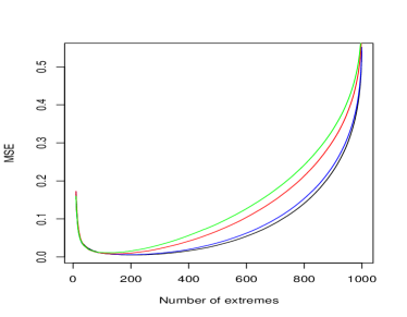
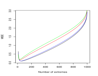
Figure 1: MSE: $\alpha=1$ (left panel), $\alpha=2$ (right panel); color codes: black - $d=0$, blue - $d=0.2$, red - $d=0.4$, green - $0.45$

We note that for $\alpha=1$, when a small number of extreme order statistics $k$ is used to build the Hill estimator, there is not much influence of the LRD parameter, and in particular the MSE is minimal for more or less the same values of $k$ through all the range of values of $d$. This is in accordance with our theoretical results. For $\alpha=2$, the influence of the memory parameter is more significant. These two features can be interpreted. First, it seems natural that the long memory effect appears when a greater number of extreme order statistics is used, since our result is of an asymptotic nature. For a small number of extremes the i.i.d. type of behaviour dominates (see $R_{n}(\cdot)$ in (33)), so the asymptotic result is seen; for a larger number of extremes, the long memory term $S_{n}$ in (33) starts to dominate. For an extremely large number of order statistics (i.e. $k\asymp n$), the bias dominates. The influence of $\alpha$ on the quality of the estimation is twofold. On one hand, the asymptotic variance of the Hill estimator is $\alpha^{2}$, so that the MSE increases with $\alpha$. Also, for very small values of $\alpha$, the peaks observed are extremely high and completely overshadow the effect of long memory.

Next, we show Hill plots for several models, since in practice one usually deals with just a single realization.

1. We consider the model $Y_{i}=\exp(\tau X_{i})Z_{i}$, where $\{X_{i}\}$ is as above a fractional Gaussian noise and $\tau=0.05$ or $2$.

2. We simulated $n=1000$ i.i.d. Pareto random variables $Z_{i}$ with parameter $\alpha=2$.

3. We simulated fractional Gaussian noise sequences $\{X_{i}\}$ with parameters $d=0$ (i.i.d. case), 0.2, 0.4, $0.45$.

4. The estimators are plotted on Figures 2 and 3. The left panel corresponds to the Hill estimator for iid Pareto random variables $\{Z_{i}\}$, and the right one for the long memory stochastic volatility process $\{Y_{i}\}$. Recall that the $Y_{i}$ are dependent asympotically Pareto random variables, so that there are two sources of bias for the Hill estimator.

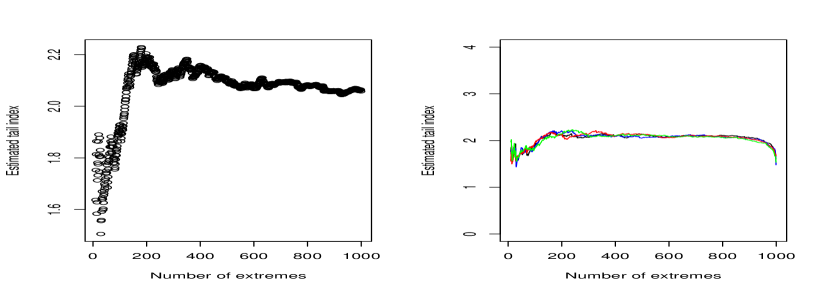
Figure 2: Hill estimator: $\alpha=2$ and Pareto iid (left panel), $\tau=0.05$ (right panel); color codes: black - $d=0$, blue - $d=0.2$, red - $d=0.4$, green - $0.45$

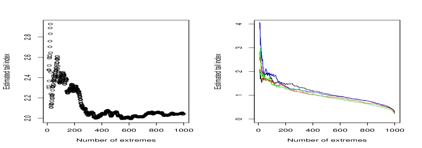
Figure 3: Hill estimator: $\alpha=2$ and Pareto iid (left panel), $\tau=1$ (right panel); color codes: black - $d=0$, blue - $d=0.2$, red - $d=0.4$, green - $0.45$

We may observe that for a small volatility parameter $\tau$ there is not too much difference between the two plots. However, if $\tau$ becomes bigger, the estimation with a large number of extremes is completely inappropriate if $d>0$, though without much influence of the strength of the dependence (i.e. increase of $d$) on this degradation. The reason is that the second order condition satisfied by the stochastic volatility model yields the same rate of convergence as in the i.i.d. case, but an increase in the variance of the Gaussian process $\{X_{t}\}$ entails a bigger bias in finite sample.

4 Proofs

4.1 Gaussian long memory sequences

Recall that each function $G(\cdot)$ in $L^{2}({\mathrm{d}}\mu)$, with $\mu({\mathrm{d}}x)=(2\pi)^{-1/2}\exp(-x^{2}/2)\,{\mathrm{d}}x$ can be expanded as

$$G(X)={\mathbb{E}}[G(X)]+\sum_{m=1}^{\infty}\frac{J(m)}{m!}H_{m}(X)\;,$$

where $J(m)={\mathbb{E}}[G(X)H_{m}(X)]$ and $X$ is a standard Gaussian random variable. Recall also that the smallest $q\geq 1$ such that $J(q)\not=0$ is called the Hermite rank of $G$. We have

$${\mathbb{E}}[G(X_{0})G(X_{k})]={\mathbb{E}}[G(X_{0})]+\sum_{m=q}^{\infty}\frac{J^{2}(m)}{m!}\,\rho_{k}^{m}\;,$$ (26)

where $\rho_{k}=\mathrm{cov}(X_{0},X_{k})$. Thus, the asymptotic behaviour of ${\mathbb{E}}[G(X_{0})G(X_{k})]$ is determined by the leading term $\rho_{n}^{q}$. In particular, if $1-q(1-H)>1/2$, which implies that $n^{2}\rho_{n}^{q}\to\infty$,

$$\mathrm{var}\left(\sum_{j=1}^{n}G(X_{j})\right)\sim\frac{J^{2}(q)}{q!}\;\frac{n^{2}\rho_{n}^{q}}{1-2q(1-H)}$$ (27)

and

$$\frac{1}{n\rho_{n}^{q/2}}\sum_{j=1}^{n}G(X_{j})\stackrel{{\scriptstyle\mbox{\tiny\rm d}}}{{\to}}J(q)L_{q}\;,$$ (28)

where

$$L_{q}=(q!(1-2q(1-H))^{-1/2}Z_{H,q}(1)$$ (29)

and $Z_{H,q}$ is the so-called Hermite or Rosenblatt process of order $q$, defined as a $q$-fold stochastic integral

$$Z_{H,q}(t)=\int_{-\infty}^{\infty}\dots\int_{-\infty}^{\infty}\frac{\mathrm{e}^{\mathrm{i}t(x_{1}+\cdots+x_{q})}-1}{x_{1}+\cdots+x_{q}}\,\prod_{i=1}^{q}x_{i}^{-H+1/2}\,W({\mathrm{d}}x_{1})\dots W({\mathrm{d}}x_{q})\;,$$

where $W$ is an independently scattered Gaussian random measure with Lebesgue control measure. For more details, the reader is referred to [20]. On the other hand, if $1-q(1-H)<1/2$ or $\{X_{j}\}$ is weakly dependent, then

$$\frac{1}{\sqrt{n}}\sum_{j=1}^{n}G(X_{j})\stackrel{{\scriptstyle\mbox{\tiny\rm d}}}{{\to}}{\cal N}(0,\Sigma_{0}^{2}),$$ (30)

where $\Sigma_{0}^{2}=\mathrm{var}(G(X_{0}))+2\sum_{j=1}^{\infty}\mathrm{cov}(G(X_{0}),G(X_{j}))<\infty$.

We will also need the following variance inequalities of [1]:

• If $1-q(1-H)>1/2$, then for any function $G$ with Hermite rank $q$ ,

  $$\mathrm{var}\left(n^{-1}\sum_{j=1}^{n}G(X_{j})\right)\leq C\rho_{n}^{q}\;\mathrm{var}(G(X_{1}))\;.$$ (31)

• If $1-q(1-H)<1/2$, then for any function $G$ with Hermite rank $q$ ,

  $$\mathrm{var}\left(n^{-1}\sum_{j=1}^{n}G(X_{j})\right)\leq Cn^{-1}\;\mathrm{var}(G(X_{1}))\;.$$ (32)

In all these cases, the constant $C$ depends only on the Gaussian process $\{X_{j}\}$ and not on the function $G$. The bounds (31) and (32) are Equation 3.10 and 2.40 in [1], respectively.

4.2 Decomposition of the tail empirical process

The main ingredient of the proof of our results will be the following decomposition. Let ${\cal X}$ be the $\sigma$-field generated by the Gaussian process $\{X_{n}\}$.

$$e_{n}(s) =\frac{1}{n\bar{F}(u_{n})}\sum_{j=1}^{n}\left\{1_{\{Y_{j}>(1+s)u_{n}\}}-{\mathbb{P}}(Y_{j}>(1+s)u_{n}|{\cal X})\right\}$$

$$\ \ \ +\frac{1}{n\bar{F}(u_{n})}\sum_{j=1}^{n}\left\{{\mathbb{P}}(Y_{j}>(1+s)u_{n}|{\cal X})-\bar{F}(u_{n})\right\}$$

$$=:R_{n}(s)+S_{n}(s)\;.$$ (33)

Conditionally on $\mathcal{X}$, $R_{n}$ is the sum of independent random variables, so it will be referred to as the i.i.d. part; the term $S_{n}$ is the partial sum process of a subordinated Gaussian process, so it will be referred to as the LRD part.

4.3 Proof of Theorem 2.2

We first give a heuristic behind the dichotomous behaviour in Theorem 2.2. Then, we prove convergence of the finite dimensional distributions of the i.i.d. and LRD parts. Finally, we prove tightness and asymptotic independence.

4.3.1 Heuristic

To present some heuristic, let us compute covariance of the tail empirical process. We have

$$\mathrm{cov}(\tilde{T}_{n}(s),\tilde{T}_{n}(t)) =\frac{1}{n\bar{F}^{2}(u_{n})}\mathrm{cov}(1_{\{Y_{1}>u_{n}(1+s)\}},1_{\{Y_{1}>u_{n}(1+t)\}})$$

$$\ \ \ +\frac{2}{n^{2}\bar{F}^{2}(u_{n})}\sum_{j=1}^{n-1}(n-j)\mathrm{cov}(1_{\{Y_{1}>u_{n}(1+s)\}},1_{\{Y_{j+1}>u_{n}(1+t)\}}\;.$$

Recall (3). If ${\mathbb{E}}[\sigma^{\alpha+\epsilon}(X_{1})]<\infty$ holds, we apply Breiman’s Lemma to both nominator and denominator to get

$$\lim_{n\to\infty}\frac{\mathrm{cov}(1_{\{Y_{1}>u_{n}(1+s)\}},1_{\{Y_{1}>u_{n}(1+t)\}})}{\bar{F}(u_{n})}\\ =\lim_{n\to\infty}\frac{{\mathbb{E}}[\sigma^{\alpha}(X_{1})]P(Z_{1}>u_{n}(1+s)\vee u_{n}(1+t))}{{\mathbb{E}}[\sigma^{\alpha}(X_{1})]P(Z_{1}>u_{n})}=T(s\vee t)\;.$$

Furthermore, if ${\mathbb{E}}[\sigma^{\alpha+\epsilon}(X_{1})\sigma^{\alpha+\epsilon}(X_{j+1})]<\infty$ holds (which is guaranteed by (8)), then a generalization of Breiman’s Lemma yields

$$\lim_{n\to\infty} \frac{\mathrm{cov}(1_{\{Y_{1}>u_{n}(1+s)\}},1_{\{Y_{j+1}>u_{n}(1+t)\}})}{\bar{F}^{2}(u_{n})}$$

$$=\lim_{n\to\infty}\frac{P(Y_{1}>u_{n}(1+s),Y_{j+1}>u_{n}(1+t))}{\bar{F}^{2}(u_{n})}-T(s)T(t)$$

$$=T(s)T(t)\left(\frac{{\mathbb{E}}[\sigma^{\alpha}(X_{1})\sigma^{\alpha}(X_{j+1})]}{{\mathbb{E}}[\sigma^{\alpha}(X_{1})]{\mathbb{E}}[\sigma^{\alpha}(X_{j+1})]}-1\right)\;.$$

Therefore, for fixed $s$ and $t$, using (27) in the case $q(1-H)<1/2$, we obtain

$$\mathrm{cov} (\tilde{T}_{n}(s),\tilde{T}_{n}(t))$$

$$=(1+o(1))\frac{T(s\vee t)}{n\bar{F}(u_{n})}$$

$$\ \ \ +(1+o(1))\frac{T(s)T(t)}{{\mathbb{E}}^{2}[\sigma^{\alpha}(X_{1})]}\frac{1}{n}\sum_{j=1}^{n-1}\left(1-\frac{j}{n}\right)\mathrm{cov}(\sigma^{\alpha}(X_{1}),\sigma^{\alpha}(X_{j+1}))$$

$$=(1+o(1))\left(\frac{T(s\vee t)}{n\bar{F}(u_{n})}+\frac{T(s)T(t)J^{2}(q)\rho_{n}^{q}}{q!(1-2q(1-H)){\mathbb{E}}^{2}[\sigma^{\alpha}(X_{1})]}\right).$$

In particular, setting $s=t$, then we conclude that the normalization factor for $e_{n}(\cdot)$ should be $\sqrt{n\bar{F}(u_{n})}$ or $\rho_{n}^{-q/2}$ depending whether $n\bar{F}(u_{n})\rho_{n}^{q}\to 0$ or $n\bar{F}(u_{n})\rho_{n}^{q}\to\infty$ holds. The asymptotic variance also suggests the form of limiting distributions in Theorem 2.2.

4.3.2 Finite dimensional limits

Let $\stackrel{{\scriptstyle\mbox{\tiny\rm d}}}{{\to}}$ denote weak convergence of finite dimensional distributions. It will be shown in Section 4.3 and 4.3, respectively, that for each $m\geq 1$ and $s_{l}\in[0,\infty)$, $l=1,\ldots,M$, $s_{1}<\cdots<s_{M}$,

$$\sqrt{n\bar{F}(u_{n})}\left(R_{n}(s_{1}),R_{n}(s_{l})-R_{n}(s_{l-1}),l=2,\ldots,M\right)\\ \stackrel{{\scriptstyle\mbox{\tiny\rm d}}}{{\to}}\left({\cal N}(0,T(s_{1})),{\cal N}(0,T(s_{l})-T(s_{l-1})),l=2,\ldots,M\right)\;,$$ (34)

where the normal random variables are independent, and

$$\rho_{n}^{-q/2}(S_{n}(s_{1}),\ldots,S_{n}(s_{M}))\stackrel{{\scriptstyle\mbox{\tiny\rm d}}}{{\to}}\frac{J(q)}{{\mathbb{E}}[\sigma^{\alpha}(X_{1})]}(T(s_{1}),\ldots,T(s_{M}))L_{q}\;,$$ (35)

if $1-q(1-H)>1/2$. On the other hand, if $1-q(1-H)<1/2$, then the second term $S_{n}(\cdot)$ is of smaller order than the first one, $R_{n}(\cdot)$.

The i.i.d. limit

Define

$$L_{n,j}(x,s) =1_{\{\sigma(x)Z_{j}>(1+s)u_{n}\}}-{\mathbb{P}}(\sigma(x)Z_{1}>(1+s)u_{n})\;.$$

Then

$$R_{n}(s)=\sum_{j=1}^{n}L_{n,j}(X_{j},s)\;.$$

Set $L_{n,j}(x)=L_{n,j}(x,0)$ and $V_{n}^{(m)}(x)={\mathbb{E}}[L_{n,j}^{m}(x)]$. Note that ${\mathbb{E}}[V_{n}^{(1)}(X_{j})]=0$ and

$$V_{n}^{(2)}(x) ={\mathbb{P}}(\sigma(x)Z_{1}>u_{n})-{\mathbb{P}}^{2}(\sigma(x)Z_{1}>u_{n})\;.$$

Let $R_{n}:=R_{n}(0)$. Therefore, for fixed $t$,

$$\log{\mathbb{E}}\left[\mathrm{e}^{\mathrm{i}t\sqrt{n\bar{F}(u_{n})}R_{n}}|{\cal X}\right]$$

$$=\sum_{j=1}^{n}\log{\mathbb{E}}\left[\exp\left(\frac{\mathrm{i}t}{\sqrt{n\bar{F}(u_{n})}}\{1_{\{Y_{j}>u_{n}\}}-{\mathbb{P}}(Y_{j}>u_{n}\mid{\cal X})\}\right)\mid{\cal X}\right]$$

$$=\sum_{j=1}^{n}\log{\mathbb{E}}\left[1-\frac{it}{\sqrt{n\bar{F}(u_{n})}}L_{n,j}(X_{j})-\frac{t^{2}}{2n\bar{F}(u_{n})}L_{n,j}^{2}(X_{j})+L_{n,j}^{3}(X_{j})O\left(\frac{1}{(n\bar{F}(u_{n}))^{3/2}}\right)\mid{\cal X}\right]$$

$$=\frac{-t^{2}}{2n\bar{F}(u_{n})}\sum_{j=1}^{n}V_{n}^{(2)}(X_{j})+o\left(\frac{1}{n\bar{F}(u_{n})}\right)\sum_{j=1}^{n}V_{n}^{(2)}(X_{j})+O\left(\frac{1}{(n\bar{F}(u_{n}))^{3/2}}\right)\sum_{j=1}^{n}|V_{n}^{(3)}(X_{j})|\;.$$ (36)

We will show that

$$\frac{1}{n\bar{F}(u_{n})}\sum_{j=1}^{n}V_{n}^{(2)}(X_{j})\stackrel{{\scriptstyle\mbox{\small\tiny p}}}{{\to}}1,$$ (37)

given that ${\mathbb{E}}[\sigma^{\alpha+\delta}(X_{1})]<\infty$. This also shows that the second term in (36) is negligible. Furthermore, since for sufficiently large $n$ and $\delta>0$ (cf. (59)),

$$|V_{n}^{(3)}(x)|\leq C{\mathbb{P}}(\sigma(x)Z_{1}>u_{n})\leq C(\sigma(x)\vee 1)^{\alpha+\delta}P(Z_{1}>u_{n})\;,$$

the expected value of the last term in (36) is

$$O\left(\frac{nP(Z_{1}>u_{n})}{(n\bar{F}(u_{n}))^{3/2}}\right){\mathbb{E}}[1\vee\sigma^{\alpha+\delta}(X_{1})]\;.$$

Consequently, the last term in (36) converges to 0 in $L^{1}$ and in probability. Therefore, on account of (37) and the negligibility, we obtain,

$$\log{\mathbb{E}}\left[\mathrm{e}^{\mathrm{i}t\sqrt{n\bar{F}(u_{n})}R_{n}}|{\cal X}\right]\stackrel{{\scriptstyle\mbox{\small\tiny p}}}{{\to}}-t^{2}/2$$ (38)

and from bounded convergence theorem we conclude (34) (for $M=1$ and $s=0$). It remains to prove (37). By Lemma 2.1, for each $j\geq 1$, $G_{n}(X_{j},s)$ converges in probability and in $L^{1}$ to $\sigma^{\alpha}(X_{j})$. Therefore,

$$\lim_{n\to\infty}{\mathbb{E}}\left[\left|\frac{1}{n}\sum_{j=1}^{n}\frac{{\mathbb{P}}(\sigma(X_{j})Z_{1}>u_{n}\mid\mathcal{X})}{{\mathbb{P}}(Z_{1}>u_{n})}-\sigma^{\alpha}(X_{j})\right|\right]=0\;.$$ (39)

Next, since $\sigma^{\alpha}(X_{j})$, $j\geq 1$, is ergodic, we have

$$\frac{1}{n}\sum_{j=1}^{n}\sigma^{\alpha}(X_{1})\stackrel{{\scriptstyle\mbox{\small\tiny p}}}{{\to}}{\mathbb{E}}[\sigma^{\alpha}(X_{1})]\;.$$ (40)

Thus, (39), (40) and Breiman’s Lemma yields

$$\frac{1}{n\bar{F}(u_{n})}\sum_{j=1}^{n}{\mathbb{P}}(\sigma(X_{j})Z_{1}>u_{n}\mid\mathcal{X})\stackrel{{\scriptstyle\mbox{\small\tiny p}}}{{\to}}1\;.$$ (41)

Write now

$$\frac{1}{n\bar{F}(u_{n})}\sum_{j=1}^{n}V_{n}^{(2)}(X_{j}) =1+o_{P}(1)+\frac{1}{n\bar{F}(u_{n})}\sum_{j=1}^{n}{\mathbb{P}}^{2}(\sigma(X_{j})Z_{1}>u_{n}\mid\mathcal{X})\;.$$

By Lemma 2.1, we have, for some $\delta>0$ small enough,

$$\frac{1}{n\bar{F}(u_{n})}\sum_{j=1}^{n}{\mathbb{P}}^{2}(\sigma(X_{j})Z_{1}>u_{n}\mid\mathcal{X})\\ \leq C{\mathbb{P}}(Z>u_{n})\frac{1}{n}\sum_{j=1}^{n}(\sigma(X_{j})\vee 1)^{2\alpha+\delta}\stackrel{{\scriptstyle\mbox{\small\tiny p}}}{{\to}}0\;.$$ (42)

This proves (37) and (34) follows with $M=1$ and $s_{1}=0$. The case of a general $M\geq 1$ is obtained analogously.

Long memory limit

Recall the definition (6) of $G_{n}(\cdot,s)$ and that $G(x)=\sigma^{\alpha}(x)$. Define

$$J_{n}(m,s)={\mathbb{E}}[H_{m}(X_{1})G_{n}(X_{1},s)],\quad J(m)={\mathbb{E}}[H_{m}(X_{1})G(X_{1})],$$

the Hermite coefficients of $G_{n}(\cdot,s)$ and $G(\cdot)$, respectively. Let $q$ be the Hermite rank of $G(\cdot)$. We write (recall Assumption (H)),

$$\sum_{j=1}^{n}(G_{n}(X_{j},s)-{\mathbb{E}}[G_{n}(X_{j},s)])$$ (43)

$$= \sum_{j=1}^{n}\sum_{m=q}^{\infty}\frac{T(s)J(m)}{m!}H_{m}(X_{j})+\sum_{j=1}^{n}\sum_{m=q}^{\infty}\frac{J_{n}(m,s)-T(s)J(m)}{m!}H_{m}(X_{j})$$

$$=: T(s)S_{n}^{*}+\tilde{S}_{n}(s)\;,$$

with $S_{n}^{*}=\sum_{j=1}^{n}G(X_{j})$. On account of Rozanov’s equality (26), we have that the variance of the second term is

$$\mathrm{var}(\tilde{S}_{n}(s)) =\sum_{i,j=1}^{n}\sum_{m=q}^{\infty}\frac{(J_{n}(m,s)-T(s)J(m))^{2}}{m!}\mathrm{cov}^{m}(X_{i},X_{j})$$

$$\leq\sum_{i,j=1}^{n}|\mathrm{cov}^{q}(X_{i},X_{j})|\sum_{m=q}^{\infty}\frac{(J_{n}(m,s)-T(s)J(m))^{2}}{m!}$$

$$=\|G_{n}(\cdot,s)-T(s)G(\cdot)\|_{L^{2}(d\mu)}^{2}\sum_{i,j=1}^{n}|\mathrm{cov}^{q}(X_{i},X_{j})|$$

$$\leq Cn^{2}\rho_{n}^{q}\,\|G_{n}(\cdot,s)-T(s)G(\cdot)\|_{L^{2}(d\mu)}^{2}\;.$$ (44)

Since ${\mathbb{E}}[\sigma^{2\alpha+\delta}(X)]<\infty$, by Lemma 2.1, $G_{n}(\cdot,s)$ converges $T(s)G(\cdot)$ in $L^{2}(d\mu)$, uniformly with respect to $s$. We conclude that the second term on the right handside of (43) is $o_{P}\left(n\rho_{n}^{q/2}\right)$, i.e. it is asymptotically smaller than the first term. Furthermore,

$$S_{n}(s)=\frac{P(Z_{1}>u_{n})}{n\bar{F}(u_{n})}\sum_{j=1}^{n}\left(G_{n}(X_{j},s)-{\mathbb{E}}[G_{n}(X_{j},s)]\right),$$ (45)

so that via (28) and (60)

$$\rho_{n}^{-q/2}S_{n}(s)\stackrel{{\scriptstyle\mbox{\tiny\rm d}}}{{\to}}\frac{J(q)T(s)}{{\mathbb{E}}[\sigma^{\alpha}(X_{1})]}L_{q}\;,$$ (46)

if $1-q(1-H)>1/2$. Consequently, (35) holds for $M=1$. The multivariate case follows immediately. On the other hand, if $1-q(1-H)<1/2$, then via (30) and (60),

$$\sqrt{n}\sup_{s\in[0,1]}S_{n}(s)\stackrel{{\scriptstyle\mbox{\tiny\rm d}}}{{\to}}\frac{1}{{\mathbb{E}}[\sigma^{\alpha}(X_{1})]}{\cal N}(0,\Sigma_{0}^{2})\;,$$

which proves negligibility with respect to the term $R_{n}(\cdot)$.

4.3.3 Asymptotic independence

In this section we prove asymptotic independence of $R_{n}(\cdot)$ and $S_{n}(\cdot)$. We will carry out a proof for the joint characteristic function of $(R_{n},S_{n})=(R_{n}(0),S_{n}(0))$. Extension to multivariate case is straightforward. On account of (38), (46) and the bounded convergence theorem, we have

$${\mathbb{E}}\left[\exp\left\{\mathrm{i}s\sqrt{n\bar{F}(u_{n})}R_{n}+\mathrm{i}t\rho_{n}^{-q/2}S_{n}\right\}\right]$$

$$= {\mathbb{E}}\left[{\mathbb{E}}[\exp\{\mathrm{i}s\sqrt{n\bar{F}(u_{n})}R_{n}\}\mid{\cal X}]\exp\left(\mathrm{i}t\rho_{n}^{-q/2}S_{n}\right)\right]$$

$$\to \exp(-s^{2}/2)\,\psi_{L_{q}}\left(\frac{J(q)}{{\mathbb{E}}[\sigma^{\alpha}(X_{1})]}\,t\right)\ \mbox{ as }n\to\infty\;,$$

where $\psi_{L_{q}}(\cdot)$ is the characteristic function of $L_{q}$. This proves asymptotic independence.

4.3.4 Tightness

In order to prove the tightness in $\mathcal{D}([0,\infty))$ endowed with Skorokhod’s $J_{1}$ topology of the sequence of processes $R_{n}^{\prime}:=\sqrt{n\bar{F}(u_{n})}R_{n}$, we apply the tightness criterion of [2, Theorem 15.4]. We must prove that for each $A>0$ and $\epsilon>0$,

$$\lim_{\delta\to 0}\limsup_{n\to\infty}{\mathbb{P}}(w_{A}^{\prime\prime}(R_{n}^{\prime},\delta)>\epsilon)=0\;,$$ (47)

where for any function $g\in\mathcal{D}([0,\infty))$,

$$w_{A}^{\prime\prime}(g,\delta)=\sup_{0\leq t_{1}\leq s\leq t_{2}\leq A}|g(s)-g(t_{1})|\wedge|g(t_{2})-g(s)|\;.$$

Since the $Y_{i}$s are independent conditionally on $\mathcal{X}$, by elementary computations similar to those that lead to [2, Inequality 13.17], we obtain that

$${\mathbb{E}}\left[|R_{n}^{\prime}(s)-R_{n}^{\prime}(t_{1})|^{2}|R_{n}^{\prime}(t_{2})-R_{n}^{\prime}(s)|^{2}\mid\mathcal{X}\right]\leq 3\{Q_{n}(t_{1})-Q_{n}(t_{2})\}^{2}\;,$$ (48)

where

$$Q_{n}(s)=\frac{1}{n\bar{F}(u_{n})}\sum_{j=1}^{n}\bar{F}_{Z}(u_{n}(1+s)/\sigma(X_{j}))\;.$$

Note that $Q_{n}(s)$ converges in probability to $T(s)$ which is a continuous decreasing function on $[0,\infty)$. Let $m\geq 1$ be an integer and set $\delta=A/2m$. Applying [2, Theorem 12.5] and using the same arguments as in the proof of [2, Theorem 15.6] (p. 129, Eq. (15.26); note that the assumed continuity of the function $F$ that appears therein is not used to obtain (15.26)), we see that the bound (48) yields, for some constant $C$ (whose numerical value may change upon each appearance),

$${\mathbb{P}}(w_{A}^{\prime\prime}(R_{n}^{\prime},\delta)>\epsilon\mid\mathcal{X}) \leq C\epsilon^{-4}\sum_{k=0}^{2m-1}\{Q_{n}(k\delta)-Q_{n}((k+2)\delta)\}^{2}$$

$$\leq C\epsilon^{-4}Q_{n}(0)\max_{0\leq k\leq 2m-1}\{Q_{n}(k\delta)-Q_{n}((k+2)\delta)\}\;.$$

Letting now $n\to\infty$ yields

$$\limsup_{n\to\infty}{\mathbb{P}}(w_{A}^{\prime\prime}(R_{n}^{\prime},\delta)>\epsilon\mid\mathcal{X})\\ \leq C\epsilon^{-4}\max_{0\leq k\leq 2m-1}\{T(k\delta)-T((k+2)\delta)\}\leq C\epsilon^{-4}\delta^{\alpha\wedge 1}\;.$$

By bounded convergence, this yields

$$\limsup_{n\to\infty}{\mathbb{P}}(w_{A}^{\prime\prime}(R_{n}^{\prime},\delta)>\epsilon)\leq C\epsilon^{-4}\delta^{\alpha\wedge 1}\;,$$

and (47) follows.

We prove now tightness of $S_{n}$. Assume first $1-q(1-H)>1/2$ and define $S_{n}^{\prime}=\rho_{n}^{-q/2}S_{n}$. Applying (31) there exists a constant $C$, which depends only on the Gaussian process $\{X_{j}\}$, such that we have, for $s\leq t$,

$$\mathrm{var}(S_{n}^{\prime}(s)-S_{n}^{\prime}(t)) \leq C\mathrm{var}(G_{n}(X_{1},s)-G_{n}(X_{1},t))$$

$$\leq C{\mathbb{E}}\left[\frac{{\mathbb{P}}^{2}(u_{n}(1+s)\leq\sigma(X_{1})Z_{1}\leq u_{n}(1+t)\mid\mathcal{X})}{{\mathbb{P}}(Z>u_{n})}\right]$$

Let the expectation in last term be denoted by $Q^{\prime}_{n}(s,t)$. By the same adaptation of the proof of [2, Theorem 15.6] as previously (see also [13] for a more general extension), we obtain, for each $A>0$, and for $\delta=A/2m$ for an integer $m\geq 1$,

$${\mathbb{P}}(w_{A}^{\prime\prime}(S_{n}^{\prime},\delta)>\epsilon)\leq C\epsilon^{-2}\sum_{k=0}^{2m-1}Q^{\prime}_{n}(2k\delta,(2k+2)\delta)\;.$$

Thus, letting $n$ tend to infinity while keeping $m$ fixed, we get

$$\limsup_{n\to\infty}{\mathbb{P}}(w_{A}^{\prime\prime}(S_{n}^{\prime},\delta)>\epsilon) \leq C\epsilon^{-2}\sum_{k=0}^{2m-1}\{(1+2k\delta)^{-\alpha}-(1+(2k+2)\delta)^{-\alpha}\}^{2}$$

$$\leq C\epsilon^{-2}\delta^{2}\sum_{k=0}^{2m-1}(1+2k\delta)^{-2\alpha-2}\leq C\epsilon^{-2}\delta\;.$$

Thus $\lim_{\delta\to 0}\limsup_{n\to\infty}{\mathbb{P}}(w_{A}^{\prime\prime}(S_{n}^{\prime},\delta)>\epsilon)=0$ and this concludes the proof of tightness.

4.4 Proof of Corollary 2.5 and Theorem 2.6

As in case of Theorem 2.2, we start some heuristic. Recall computation from Section 4.3.1 and the form of the limiting distribution $w-T\cdot w(0)$. Then

$$\mathrm{var}(\hat{T}_{n}(s))=(1+o(1))\mathrm{var}(\tilde{T}_{n}(s)-T(s)\tilde{T}_{n}(0))$$

$$= (1+o(1))\frac{1}{n\bar{F}(u_{n})}T(s)(1-T(s))+o(1)T^{2}(s)\rho_{n}^{q}.$$

This suggests that in LRD zone $\rho_{n}^{-q/2}\hat{T}_{n}(\cdot)$ converges to 0.

To prove it formally, denote $\bar{T}_{n}=T_{n}-T$ and $\xi_{n}=\frac{Y_{n-k:n}-u_{n}}{u_{n}}=\tilde{T}_{n}^{\leftarrow}(1)$. Then $\tilde{T}_{n}(\xi_{n})=1$, and we have

$$1=e_{n}(\xi_{n})+T_{n}(\xi_{n})=e_{n}(\xi_{n})+\bar{T}_{n}(\xi_{n})+T(\xi_{n})\;.$$

Thus,

$$T(\xi_{n})-1=-e_{n}(\xi_{n})-\bar{T}_{n}(\xi_{n})\;.$$ (49)

For any $s\geq 0$, $\hat{T}_{n}(s)=\tilde{T}_{n}(s+\xi_{n}(1+s))$ and $T(s+\xi_{n}(1+s))=T(s)T(\xi_{n})$, thus

$$\hat{e}_{n}^{*}(s) =e_{n}(s+\xi_{n}(1+s))+\bar{T}_{n}(s+\xi_{n}(1+s))+T(s+\xi_{n}(1+s))-T(s)$$

$$=e_{n}(s+\xi_{n}(1+s))+T(s)\{T(\xi_{n})-1\}+\bar{T}_{n}(s+\xi_{n}(1+s))\;.$$

Plugging (49) into this decomposition of $\hat{e}_{n}^{*}$, we get

$$\hat{e}_{n}^{*}(s) =e_{n}(s+\xi_{n}(1+s))-T(s)e_{n}(\xi_{n})+\bar{T}_{n}(s+\xi_{n}(1+s))-T(s)\bar{T}_{n}(\xi_{n})\;.$$ (50)

In order to prove Corollary 2.5, we write

$$w_{n}\hat{e}_{n}^{*}(s) =w_{n}\{e_{n}(s+\xi_{n}(1+s))-T(s)e_{n}(\xi_{n})\}+O(w_{n}\|T_{n}-T\|_{\infty})\;.$$ (51)

Since the convergence in Theorem 2.2 is uniform, and by Corollary 2.4 $\xi_{n}=o_{P}(1)$, the first term in (51) converges in $D([0,\infty))$ to $w-T\cdot w(0)$. Under the second order condition (14), the second term is $o(1)$. This concludes the proof of Theorem 2.5.

We now prove Theorem 2.6. In order to study the second-order asymptotics of $w_{n}\hat{e}_{n}^{*}(s)$, we need precise expansion for $e_{n}(s+\xi_{n}(1+s))$ and $e_{n}(\xi)$. For this we will use the expansions of the tail empirical process in Section 4.3.2. Since $\bar{F}(u_{n})=k/n$, using (33), (43) and (45), we have

$$e_{n}(s)=R_{n}(s)+\frac{\bar{F}_{Z}(u_{n})}{n\bar{F}(u_{n})}\,T(s)S_{n}^{*}+\frac{\bar{F}_{Z}(u_{n})}{n\bar{F}(u_{n})}\tilde{S}_{n}(s)\;,$$ (52)

which, noting again that $T(s+\xi_{n}(1+s))=T(s)T(\xi_{n})$, yields

$$e_{n}(s+\xi_{n}(1+s))-T(s)e_{n}(\xi_{n}) =R_{n}(s+\xi_{n}(1+s))-T(s)R_{n}(\xi_{n})$$

$$\ \ \ +\frac{\bar{F}_{Z}(u_{n})}{n\bar{F}(u_{n})}\{\tilde{S}_{n}(s+\xi_{n}(1+s))-T(s)\tilde{S}_{n}(\xi_{n})\}\;$$

and

$$\hat{e}_{n}^{*}(s)=R_{n}(s+\xi_{n}(1+s))-T(s)R_{n}(\xi_{n})\\ +\frac{\bar{F}_{Z}(u_{n})}{n\bar{F}(u_{n})}\{\tilde{S}_{n}(s+\xi_{n}(1+s))-T(s)\tilde{S}_{n}(\xi_{n})\}+\bar{T}_{n}(s+\xi_{n}(1+s))-T(s)\bar{T}_{n}(\xi_{n})\;.$$ (53)

Similarly to (44), and utilising $\bar{F}_{Z}(u_{n})/\bar{F}(u_{n})=O(1)$,

$$\mathrm{var}\left(\frac{\bar{F}_{Z}(u_{n})}{n\bar{F}(u_{n})}\tilde{S}_{n}(s)\right)\leq C\{\rho_{n}^{q}\vee\ell_{1}(n)n^{-1}\}\|G_{n}(\cdot,s)-T(s)G(\cdot)\|_{L^{2}(\mu)}^{2}\;.$$

Using the second order Assumption (SO) through (22), we obtain

$$\mathrm{var}\left(\frac{\bar{F}_{Z}(u_{n})}{n\bar{F}(u_{n})}\tilde{S}_{n}(s)\right)=O\left(\{\rho_{n}^{q}\vee\ell_{1}(n)n^{-1}\}\eta^{*}(u_{n})^{2}\right)=o\left(\eta^{*}(u_{n})^{2}\right)\;.$$ (54)

Using (52) in the representation (50) and since Proposition 2.8 implies that $\|T_{n}-T\|_{\infty}=O(\eta^{*}(u_{n}))$, we obtain:

$$\hat{e}_{n}^{*}(s) =R_{n}(s+\xi_{n}(1+s))-T(s)R_{n}(\xi_{n})+O_{P}(\eta^{*}(u_{n}))\;.$$

Since we have already proved that the convergence of $\sqrt{k}R_{n}$ is uniform, we obtain that $\sqrt{k}e_{n}^{*}$ converges in the sense of finite dimensional distribution to $B\circ T$, where $B$ is the Brownian bridge, if the second order condition (19) holds. To prove tightness, we only have to prove that $k^{1/2}n^{-1}S_{n}$ converges uniformly to zero on compact sets. For $s\geq 0$ and $x\in\mathbb{R}$, denote $\bar{G}_{n}(x,s)=G_{n}(x,s)-T(s)G(x)$ and recall that we have shown in Section 4.3.4 that

$$n^{-2}\mathrm{var}(\tilde{S}_{n}(s)-\tilde{S}_{n}(s^{\prime})) \leq C\|\bar{G}_{n}(\cdot,s_{2})-\bar{G}_{n}(\cdot,s_{1})\|_{L^{2}(d\mu)}^{2}\;.$$

Applying (63), we get

$$n^{-2}\mathrm{var}(\tilde{S}_{n}(s)-\tilde{S}_{n}(s^{\prime}))\leq C(\eta^{*}(u_{n}))^{2}{\mathbb{E}}\left[(\sigma(x)\vee 1)^{2\alpha(\beta+1)+\epsilon}\right](s-s^{\prime})^{2}\;,$$ (55)

which proves that $k^{1/2}n^{-1}\tilde{S}_{n}$ converges uniformly to zero on compact sets.

4.5 Proof of Corollary 2.7

Using the decomposition (53), and the identity $\int_{0}^{\infty}(1+s)^{-1}\,T(s)\,{\mathrm{d}}s=\gamma$, we have

$$\hat{\gamma}_{n}-\gamma =\int_{0}^{\infty}\frac{\hat{e}_{n}^{*}(s)}{1+s}\,{\mathrm{d}}s=\int_{0}^{\infty}\frac{R_{n}(s+\xi_{n}(1+s))}{1+s}\,{\mathrm{d}}s-\gamma R_{n}(\xi_{n})$$

$$+\frac{\bar{F}_{Z}(u_{n})}{n\bar{F}(u_{n})}\int_{0}^{\infty}\frac{\tilde{S}_{n}(s+\xi_{n}(1+s))}{1+s}\,{\mathrm{d}}s-\gamma\frac{\bar{F}_{Z}(u_{n})}{n\bar{F}(u_{n})}\tilde{S}_{n}(\xi_{n})$$ (56)

$$+\int_{0}^{\infty}\frac{\bar{T}_{n}(s+\xi_{n}(1+s))}{1+s}\,{\mathrm{d}}s-\gamma\bar{T}_{n}(\xi_{n})\;.$$ (57)

We must prove that the terms in (56) and (57) are $O_{P}(\eta^{*}(u_{n}))$ and that

$$\sqrt{k}\int_{0}^{\infty}(1+s)^{-1}R_{n}(s+\xi_{n}(1+s))\,{\mathrm{d}}s\stackrel{{\scriptstyle\mbox{\tiny\rm d}}}{{\to}}\int_{0}^{\infty}\frac{W\circ T(s)}{1+s}\,{\mathrm{d}}s=\gamma\int_{0}^{1}\frac{W(t)}{t}\,{\mathrm{d}}t\;.$$ (58)

To prove (58), we follow the lines of [18, Section 9.1.2]. We must prove that we can apply continuous mapping. To do this, it suffices to establish that for any $\delta>0$ we have

$$\lim_{M\to\infty}\limsup_{n\to\infty}A_{n,M}=0\;,$$

where

$$A_{n,M}={\mathbb{P}}\left(\sqrt{k}\int_{M}^{\infty}\left|\frac{1}{k}\sum_{j=1}^{n}\left(1_{\{Y_{j}>u_{n}s\}}-P\left(Y_{j}>u_{n}s|{\cal X}\right)\right)\right|\frac{ds}{s}>\delta\right)\;.$$

By Markov’s inequality, conditional independence and Potter’s bound [3, Theorem 1.5.6] , we have, for some $\epsilon>0$,

$$A_{n,M}\leq C\frac{\sqrt{n}}{\sqrt{k}}\int_{M}^{\infty}\frac{{\mathbb{P}}^{1/2}(Y>u_{n}s)}{s}\,{\mathrm{d}}s\leq C\,\sqrt{\frac{n\bar{F}(u_{n})}{k}}\int_{M}^{\infty}s^{-1-\alpha/2+\epsilon}\,{\mathrm{d}}s\leq CM^{-\alpha/2+\epsilon}\to 0$$

as $M\to\infty$, since $k=n\bar{F}(u_{n})$. This proves (58). To get a bound for (57), we use (61) which yields, for all $t\geq 0$,

$$|\bar{T}_{n}(t)|\leq C\eta^{*}(u_{n})(1+t)^{-\alpha+\rho\pm\epsilon}\;.$$

Thus $\bar{T}_{n}(\xi_{n})=O_{P}(\eta^{*}(u_{n}))$ and $|\bar{T}_{n}(s+\xi_{n}(1+s))|\leq C\eta^{*}(u_{n})(1+s)^{-\alpha+\rho+\epsilon}(1+\xi_{n})^{-\alpha}$, thus

$$\int_{0}^{\infty}\frac{|T_{n}(s+\xi_{n}(1+s))|}{1+s}\,{\mathrm{d}}s=O_{P}(\eta^{*}(u_{n}))\;.$$

We finally bound (56).

$$\int_{0}^{\infty}\frac{n^{-1}\tilde{S}_{n}(s+\xi_{n}(1+s))}{1+s}\,{\mathrm{d}}s =\int_{\xi_{n}}^{\infty}\frac{n^{-1}\tilde{S}_{n}(u)}{1+u}\,{\mathrm{d}}u\;.$$

Since $\xi_{n}=o_{P}(1)$, we can write

$${\mathbb{P}}\left(k^{1/2}\int_{\xi_{n}}^{\infty}\frac{n^{-1}\tilde{S}_{n}(u)}{1+u}\,{\mathrm{d}}u>\epsilon\right) \leq{\mathbb{P}}(\xi_{n}>1)+{\mathbb{P}}\left(k^{1/2}\int_{1}^{\infty}\frac{n^{-1}|\tilde{S}_{n}(u)|}{1+u}\,{\mathrm{d}}u>\epsilon\right)$$

$$\leq o(1)+\frac{k^{1/2}}{n\epsilon}\int_{1}^{\infty}\frac{{\mathbb{E}}^{1/2}[\tilde{S}_{n}^{2}(s)]}{1+s}\;{\mathrm{d}}s$$

Applying (44) and (70) yields

$$\int_{1}^{\infty}\frac{n^{-1}{\mathbb{E}}^{1/2}[\tilde{S}_{n}^{2}(s)]}{1+s}\,{\mathrm{d}}s \leq C\rho_{n}^{q/2}\eta^{*}(u_{n})\int_{0}^{\infty}s^{-\alpha(\beta+1)/2+\epsilon-1}\,{\mathrm{d}}s=o_{P}(k^{-1/2})\;.$$

Thus the first term in (56) is $o_{P}(k^{-1/2})$, and so is the second term since $k^{1/2}n^{-1}\tilde{S}_{n}$ converges uniformly to zero on compact sets. This concludes the proof of Corollary 2.7.

4.6 Second order regular variation

The main tool in the study of the tail of the product $YZ$ is the following bound. For any $\epsilon>0$, there exists a constant $C$ such that, for all $y>0$,

$$\frac{{\mathbb{P}}(yZ_{1}>x)}{{\mathbb{P}}(Z_{1}>x)}\leq C(1\vee y^{\alpha+\epsilon})\;.$$ (59)

This bound is trivial if $y<1$ and follows from Potter’s bounds if $y>1$.

Proof of Lemma 2.1.

By Breiman’s Lemma, we know that for any sequence $u_{n}$ such that $u_{n}\to\infty$,

$$\lim_{n\to\infty}G_{n}(x,s)=\lim_{n\to\infty}\frac{{\mathbb{P}}(\sigma(x)Z_{1}>(1+s)u_{n})}{{\mathbb{P}}(Z>u_{n})})=\sigma^{\alpha}(x)(1+s)^{-\alpha}=\sigma^{\alpha}(x)T(s)\;.$$ (60)

If ${\mathbb{E}}[\sigma^{\alpha+\epsilon}(X)]<\infty$, then the bound (59) implies that the convergence (60) holds in $L^{p}(\mu)$ for any $p$ such that $p\alpha<\alpha+\epsilon$, uniformly with respect to $s$, i.e.

$$\lim_{n\to\infty}{\mathbb{E}}[\sup_{s\geq 0}|G_{n}(X,s)-\sigma^{\alpha}(X)T(s)|^{p}]=0\;.$$

∎

Before proving Proposition 2.8, we need the following lemma which gives a non uniform rate of convergence.

Lemma 4.1.

If (4), (16) and (17) hold, if $\eta^{*}$ is regularly varying at infinity with index $\rho$, for some $\rho\leq 0$, then for any $\epsilon>0$, there exists a constant $C$ such that

$$\forall t\geq 1\;,\ \ \forall z>0\;,\ \ \left|\frac{{\mathbb{P}}(Z>zt)}{{\mathbb{P}}(Z>t)}-z^{-\alpha}\right|\leq C\eta^{*}(t)z^{-\alpha+\rho}(z\vee z^{-1})^{\epsilon}\;.$$ (61)

Proof.

Since $\eta^{*}$ is decreasing, using the bound $|\mathrm{e}^{u}-1|\leq u\mathrm{e}^{u_{+}}$ with $u_{+}=\max(u,0)$, we have, for all $z>0$,

$$\left|\frac{{\mathbb{P}}(Z>zt)}{{\mathbb{P}}(Z>t)}-z^{-\alpha}\right| =z^{-\alpha}\left|\exp\int_{1}^{z}\frac{\eta(ts)}{s}\,{\mathrm{d}}s-1\right|$$

$$\leq Cz^{-\alpha}\int_{z\wedge 1}^{z\vee 1}\frac{\eta^{*}(st)}{s}\;{\mathrm{d}}s\;\exp\int_{z\wedge 1}^{z\vee 1}\frac{\eta^{*}(st)}{s}\;{\mathrm{d}}s$$

$$\leq Cz^{-\alpha}\log(z)\,\eta^{*}(t(z\wedge 1))\;\exp\int_{z\wedge 1}^{z\vee 1}\frac{\eta^{*}(st)}{s}\;{\mathrm{d}}s$$

$$\leq Cz^{-\alpha}(z\wedge 1)^{\rho-\epsilon/2}\,\eta^{*}(t)\;\exp\int_{z\wedge 1}^{z\vee 1}\frac{\eta^{*}(st)}{s}\;{\mathrm{d}}s\;.$$ (62)

We now distinguish three cases. Recall that $\eta^{*}$ is decreasing.

• If $z\geq 1$, then $z\to\exp\int_{1}^{z}s^{-1}{\eta^{*}(s)}\,{\mathrm{d}}s$ is a slowly varying function by Karamata’s representation Theorem, and is $O(z^{\epsilon/2})$ for any $\epsilon>0$. Plugging this bound into (62) yields (61).

• If $z<1$ and $tz\geq 1$, then

  $$\exp\int_{z}^{1}\frac{\eta^{*}(st)}{s}\;{\mathrm{d}}s=\exp\int_{1}^{1/z}\frac{\eta^{*}(stz)}{s}\,{\mathrm{d}}s\leq\exp\int_{1}^{1/z}\frac{\eta^{*}(s)}{s}\,{\mathrm{d}}s=O(z^{-\epsilon/2})$$

  for any $\epsilon>0$ by the same argument as above and this yields (61).

• If $tz<1$, then $t^{r}\leq z^{-r}$ for any $r>0$ and $t^{\rho-\epsilon}=O(\eta^{*}(t))$ for any $\epsilon>0$. Thus

  $$\left|\frac{{\mathbb{P}}(Z>zt)}{{\mathbb{P}}(Z>t)}-z^{-\alpha}\right| \leq\frac{1}{{\mathbb{P}}(Z>t)}+z^{-\alpha}\leq Ct^{\alpha+\epsilon/2}+z^{-\alpha}\leq Cz^{-\alpha-\epsilon/2}$$

  $$\leq Cz^{-\alpha+\rho-\epsilon}t^{\rho-\epsilon/2}\leq Cz^{-\alpha+\rho-\epsilon}\eta^{*}(t)\;.$$

This concludes the proof of (61). ∎

The following bound is used in the proof of prove Theorem 2.6.

Lemma 4.2.

If (4), (16) and (17) hold, if $\eta^{*}$ is regularly varying at infinity with index $\rho$, for some $\rho\leq 0$, then there exists a constant $C$ such that for all $t\geq 1$ and $b>a>0$,

$$\left|\frac{{\mathbb{P}}(at<Z\leq bt)}{{\mathbb{P}}(Z>t)}-(a^{-\alpha}-b^{-\alpha})\right| \leq C\eta^{*}(t)(a\wedge 1)^{-\alpha+\rho-\epsilon}(b-a)\;.$$ (63)

Proof.

The bound (63) follows from the following one and (59) applied to the function $\eta^{*}$.

$$\left|\frac{{\mathbb{P}}(at<Z\leq bt)}{{\mathbb{P}}(Z>t)}-(a^{-\alpha}-b^{-\alpha})\right| \leq C\eta^{*}((a\wedge 1)t)(a\wedge 1)^{-\alpha-1-\epsilon}(b-a)$$ (64)

Let $\ell$ be the function slowly varying at infinity that appears in (4), defined on $[0,\infty)$ by $\ell(t)=t^{\alpha}{\mathbb{P}}(Z>t)$. Assumption (SO) implies that

$$\ell(t)=\ell(1)\exp\int_{1}^{t}\eta(s)\;\frac{{\mathrm{d}}s}{s}$$ (65)

where the function $\eta$ is measurable and bounded. This implies that the function $\ell$ is the solution of the equation

$$\ell(t)=\ell(1)+\int_{1}^{t}\eta(s)\ell(s)\;\frac{{\mathrm{d}}s}{s}\;.$$ (66)

Conversely, if $\ell$ satisfies (66) then (65) holds. We first prove the following useful bound. For any $\epsilon>0$, there exists a constant $C$ such that for any $t\geq 1$ and all $a>0$,

$$\frac{\ell(at)}{\ell(t)}\leq Ca^{\pm\epsilon}\;,$$ (67)

where we denote $a^{\pm\epsilon}=\max(a^{\epsilon},a^{-\epsilon})$. Indeed, if $at\geq 1$, then, $\eta^{*}$ being decreasing, we have

$$\frac{\ell(at)}{\ell(t)}\leq C\exp\int_{a\wedge 1}^{a\vee 1}\frac{\eta^{*}(ts)}{s}\,{\mathrm{d}}s\leq C\exp\int_{1}^{a\vee(1/a)}\frac{\eta^{*}(ts)}{s}\,{\mathrm{d}}s\leq Ca^{\pm\epsilon}\;,$$

since the latter function is slowly varying by Karamata’s representation theorem. If $at<1$, then $\ell(at)\leq 1$ and $\ell^{-1}(t)=o(t^{\epsilon})=o(a^{-\epsilon})$. This proves (67). Next, applying (66) and (67), for any $\epsilon>0$ and $0<a<b$, we have

$$\left|\frac{\ell(bt)}{\ell(at)}-1\right| = \left|\int_{a}^{b}\eta(st)\,\frac{\ell(st)}{\ell(at)}\,\frac{{\mathrm{d}}s}{s}\right|\leq Ca^{\pm\varepsilon}\left|\int_{a}^{b}\eta(st)\,\frac{\ell(st)}{\ell(t)}\,\frac{{\mathrm{d}}s}{s}\right|$$ (68)

$$\leq C\eta^{*}(at)\int_{a}^{b}s^{\pm 2\epsilon-1}\;{\mathrm{d}}s\leq C\eta^{*}(at)\,a^{\pm\epsilon-1}(b-a)\;.$$

Applying (67) and (68), we also obtain

$$\left|\frac{\ell(at)}{\ell(t)}-1\right| \leq C\eta^{*}((a\wedge 1)t)\,a^{\pm\epsilon}\;.$$ (69)

For $\epsilon>0$ and $0<a<b$, we have

$$\frac{{\mathbb{P}}(at<Z\leq bt)}{{\mathbb{P}}(Z>t)}-(a^{-\alpha}-b^{-\alpha}) =a^{-\alpha}\left\{\frac{\ell(at)}{\ell(t)}-1\right\}-b^{-\alpha}\left\{\frac{\ell(bt)}{\ell(t)}-1\right\}\$$

$$=(a^{-\alpha}-b^{-\alpha})\left\{\frac{\ell(at)}{\ell(t)}-1\right\}-b^{-\alpha}\frac{\ell(at)}{\ell(t)}\left\{\frac{\ell(bt)}{\ell(at)}-1\right\}\;,$$

which yields

$$\left|\frac{{\mathbb{P}}(at<Z\leq bt)}{{\mathbb{P}}(Z>t)}-(a^{-\alpha}-b^{-\alpha})\right| \leq C\eta^{*}((a\wedge 1)t)a^{\alpha-1\pm\epsilon}(b-a)\;.$$

∎

Proof of Proposition 2.8.

Define the function $\bar{\sigma}$ by $\bar{\sigma}(x)=\sigma(x)\vee 1$. Applying (61) with $(1+s)/\sigma(x)$ instead of $z$ and $u_{n}$ for $t$, we get

$$\left|G_{n}(x,s)-\sigma^{\alpha}(x)T(s)\right| =\left|\frac{{\mathbb{P}}(\sigma(x)Z>u_{n}(1+s))}{{\mathbb{P}}(Z>u_{n})}-\sigma^{\alpha}(x)T(s)\right|$$

$$\leq C\eta^{*}(u_{n})\bar{\sigma}(x)^{\alpha(\beta+1)+\epsilon}(1+s)^{-\alpha(\beta+1)+\epsilon}\;.$$ (70)

This implies, for all $p$ such that ${\mathbb{E}}[\sigma^{p\alpha(\beta+1)+\epsilon}(X)]<\infty$, that

$${\mathbb{E}}\left[\sup_{s\geq 1}|G_{n}(X,s)-T(s)\sigma^{\alpha}(X)|^{p}\right]=O(\{\eta^{*}(u_{n})\}^{p})\;.$$

This proves (22) which in turn implies (21) since $T_{n}(s)=\frac{\bar{F}(u_{n})}{\bar{F}_{Z}(u_{n})}{\mathbb{E}}[G_{n}(X,s)]$. In order to prove that $\bar{F}_{Y}\in 2RV(-\alpha,\eta^{*})$, denote $\tilde{\ell}(y)=y^{\alpha}{\mathbb{P}}(Y>y)$. We will prove that there exists a measurable function $\tilde{\eta}$ such that (66) holds with $\tilde{\ell}$ and $\tilde{\eta}$. Denote $\xi=\sigma(X)$. Applying (66) and using the independence of $\xi$ and $Z$, we have

$$\tilde{\ell}(y) ={\mathbb{E}}[\xi^{\alpha}\ell(y/\sigma)]=\ell(1){\mathbb{E}}[\xi^{\alpha}]+{\mathbb{E}}\left[\xi^{\alpha}\int_{1}^{y/\xi}\eta(s)\ell(s)\frac{{\mathrm{d}}s}{s}\right]$$

$$=\ell(1){\mathbb{E}}[\xi^{\alpha}]+{\mathbb{E}}\left[\xi^{\alpha}\int_{\xi}^{y}\eta(s/\xi)\ell(s/\xi)\frac{{\mathrm{d}}s}{s}\right]$$

$$={\mathbb{E}}\left[\xi^{\alpha}\left\{\ell(1)-\int_{1}^{\xi}\eta(s/\xi)\ell(s/\xi)\frac{{\mathrm{d}}s}{s}\right\}\right]+{\mathbb{E}}\left[\xi^{\alpha}\int_{1}^{y}\eta(s/\xi)\ell(s/\xi)\frac{{\mathrm{d}}s}{s}\right]$$

$$={\mathbb{E}}\left[\xi^{\alpha}\left\{\ell(1)+\int_{1/\xi}^{1}\eta(s)\ell(s)\frac{{\mathrm{d}}s}{s}\right\}\right]+\int_{1}^{y}{\mathbb{E}}[\xi^{\alpha}\eta(s/\xi)\ell(s/\xi)]\frac{{\mathrm{d}}s}{s}$$

$$={\mathbb{E}}\left[\xi^{\alpha}\ell(1/\xi)\right]+\int_{1}^{y}{\mathbb{E}}[\xi^{\alpha}\eta(s/\xi)\ell(s/\xi)]\frac{{\mathrm{d}}s}{s}=\tilde{\ell}(1)+\int_{1}^{t}\tilde{\eta}(s)\tilde{\ell}(s)\frac{{\mathrm{d}}s}{s}\;,$$

where we have defined

$$\tilde{\eta}(s)=\frac{{\mathbb{E}}[\xi^{\alpha}\eta(s/\xi)\ell(s/\xi)]}{{\mathbb{E}}[\xi^{\alpha}\ell(s/\xi)]}=\frac{{\mathbb{E}}[\xi^{\alpha}\eta(s/\xi)\ell(s/\xi)/\ell(s)]}{{\mathbb{E}}[\xi^{\alpha}\ell(s/\xi)/\ell(s)]}\;.$$

The denominator of the last expression is bounded away from zero. Indeed, let $\epsilon>0$ be such that ${\mathbb{P}}(\xi\geq\epsilon)>0$. Then

$${\mathbb{E}}[\xi^{\alpha}\ell(s/\xi)/\ell(s)]=\frac{{\mathbb{P}}(\xi Z>s)}{{\mathbb{P}}(Z>s)}\geq\frac{{\mathbb{P}}(\xi\geq\epsilon){\mathbb{P}}(Z>s/\epsilon)}{{\mathbb{P}}(Z>s)}\;.$$

Since $Z$ has a regularly varying tail, it holds that $\inf_{s\geq 0}{\mathbb{P}}(Z>s/\epsilon)/{\mathbb{P}}(Z>s)>0$. This proves our claim. Thus, applying (59) with the regularly varying function $\eta^{*}$, we get, for $\epsilon>0$ such that $\exp[\xi^{\alpha-\rho+\epsilon}]<\infty$,

$$|\tilde{\eta}(s)|\leq C\eta^{*}(s)\,{\mathbb{E}}[\xi^{\alpha}\{\eta^{*}(s/\xi)/\eta^{*}(s)\}\{\ell(s/\xi)/\ell(s)\}]\leq C\eta^{*}(x)\,{\mathbb{E}}[\xi^{\alpha}(\xi\vee 1)^{-\rho+\epsilon}]\;.$$

Thus $\tilde{\ell}$ satisfies equation (66) with $\tilde{\eta}$ such that $|\eta|\leq C\eta^{*}$, thus $Y\in 2RV(-\alpha,\eta^{*})$. ∎

References

- [1] Miguel A. Arcones. Limit theorems for nonlinear functionals of a stationary Gaussian sequence of vectors. The Annals of Probability, 22(4):2242–2274, 1994.
- [2] Patrick Billingsley. Convergence of probability measures. New York, Wiley, 1968.
- [3] Nicholas H. Bingham, Charles M. Goldie, and Jozef L. Teugels. Regular variation. Cambridge University Press, Cambridge, 1989.
- [4] F. Jay Breidt, Nuno Crato, and Pedro de Lima. The detection and estimation of long memory in stochastic volatility. Journal of Econometrics, 83(1-2):325–348, 1998.
- [5] L. Breiman. On some limit theorems similar to the arc-sin law. Teor. Verojatnost. i Primenen., 10:351–360, 1965.
- [6] Richard A. Davis and Thomas Mikosch. Point process convergence of stochastic volatility processes with application to sample autocorrelation. Journal of Applied Probability, 38A:93–104, 2001. Probability, statistics and seismology.
- [7] Rohit Deo, Mengchen Hsieh, Clifford M. Hurvich, and Philippe Soulier. Long memory in nonlinear processes. In Dependence in probability and statistics, volume 187 of Lecture Notes in Statist., pages 221–244. Springer, New York, 2006.
- [8] Holger Drees. Optimal rates of convergence for estimates of the extreme value index. The Annals of Statistics, 26(1):434–448, 1998.
- [9] Holger Drees. Weighted approximations of tail processes for -mixing random variables. The Annals of Applied Probability, 10(4):1274–1301, 2000.
- [10] Holger Drees. Tail empirical processes under mixing conditions. In Empirical process techniques for dependent data, pages 325–342. Birkhäuser Boston, Boston, MA, 2002.
- [11] Holger Drees. Extreme quantile estimation for dependent data, with applications to finance. Bernoulli, 9(4):617–657, 2003.
- [12] John H. J. Einmahl. Limit theorems for tail processes with application to intermediate quantile estimation. Journal of Statistical Planning and Inference, 32(1):137–145, 1992.
- [13] Christian Genest, Kilani Ghoudi, and Bruno Rémillard. A note on tightness. Statistics and Probability Letters, 27(4):331–339, 1996.
- [14] Liudas Giraitis and Donatas Surgailis. Central limit theorem for the empirical process of a linear sequence with long memory. Journal of Statistical Planning and Inference, 80(1-2):81–93, 1999.
- [15] Hwai-Chung Ho and Tailen Hsing. Limit theorems for functionals of moving averages. The Annals of Probability, 25(4):1636–1669, 1997.
- [16] Rafał Kulik. Sums of extreme values of subordinated long-range dependent sequences: moving averages with finite variance. Electronic Journal of Probability, 13(32): 961–979, 2008.
- [17] Rafal Kulik. Empirical process of long-range dependent sequences when parameters are estimated. Journal of Statistical Planning and Inference, 139(2):287–294, 2009.
- [18] Sidney I. Resnick. Heavy-tail phenomena. Springer Series in Operations Research and Financial Engineering. Springer, New York, 2007. Probabilistic and statistical modeling.
- [19] Holger Rootzén. Weak convergence of the tail empirical process for dependent sequences. Stochastic Processes and their Applications, 119(2):468–490, 2009.
- [20] Murad S. Taqqu. Fractional Brownian motion and long-range dependence. In Theory and applications of long-range dependence, pages 5–38. Birkhäuser Boston, Boston, MA, 2003.
- [21] Ward Whitt. Stochastic-process limits. Springer Series in Operations Research. Springer-Verlag, New York, 2002. An introduction to stochastic-process limits and their application to queues.