The Interior Dynamics of Water Planets

Abstract

The ever-expanding catalog of detected super-Earths calls for theoretical studies of their properties in the case of a substantial water layer. This work considers such water planets with a range of masses and water mass fractions ($2-5\,M_{Earth}$, $0.02-50\%\,H_{2}O$). First, we model the thermal and dynamical structure of the near-surface for icy and oceanic surfaces, finding separate regimes where the planet is expected to maintain a subsurface liquid ocean and where it is expected to exhibit ice tectonics. Newly discovered exoplanets may be placed into one of these regimes given estimates of surface temperature, heat flux, and gravity. Second, we construct a parametrized convection model for the underlying ice mantle of higher ice phases, finding that materials released from the silicate - iron core should traverse the ice mantle on the time scale of $0.1$ to a hundred megayears. We present the dependence of the overturn times of the ice mantle and the planetary radius on total mass and water mass fraction. Finally, we discuss the implications of these internal processes on atmospheric observables.

1 Introduction

The discoveries of planetary systems around other stars has now led us into the realm of planets in the mass range from about 2 to 10-15 $M_{Earth}$, which are expected to be terrestrial in nature and unlike the gas giants in our Solar System. This new type of planets has been collectively called "super-Earths" (Melnick et al., 2001). Initially, mass is the main physical parameter available. As such, observers who have discovered nearly a dozen such planets to date (e.g., Mayor et al. 2009 and references therein) cannot yet distinguish between the various interior structures that are expected in this mass range, i.e. water-rich, dry, or gas-dominated (’mini Neptunes’) types. This is expected to change shortly, with the first super-Earth discovered in transit, CoRoT-7b (Leger et al., 2009), and many more anticipated to come from NASA’s Kepler mission, affording derivation of mean densities and bulk composition.

Theoretical models of planet formation anticipate large numbers of water-rich super-Earths (Ida and Lin 2004; Raymond et al. 2004; Kennedy et al. 2006). In this paper we define as water planet any planet in the super-Earth mass range composed of $>10\%$ $H_{2}O$ by mass around a silicate - metal core and that lacks a significant gas ($H$ and $He$) layer.

Water planets were proposed by Kuchner (2003) and Leger et al. (2004), and modeled with detailed $T$-dependent equations of state (EOSs) by Valencia et al. (2007a), Sotin et al. (2007), and Grasset et al. (2009). Mass-radius relations have been computed to help distinguish between the different types of super-Earths when observations become available (e.g. Valencia et al. 2007b, Fortney et al. 2007, Seager et al. 2007, and Selsis et al. 2007). Ehrenreich and Cassan (2007) and Tajika (2008) considered cold, ice-covered water planets. With the prospect of high-quality observational data on water planets becoming available (CoRoT, Kepler, JWST), there is strong motivation to take the modeling described above to a new level and focus on the geophysical details of the water layer(s), which is the goal of this work.

This work begins by constructing hydrostatic models that take into account the effect of ice phase transitions up to Ice X. We model nine ocean planets with total mass ranging from $2$ to $10\,M_{Earth}$ and water mass percents from $0.02\%$ (Earth-like) to $50\%$. Section 2 explains the creation of these models.

Section 3 presents a pair of models to constrain the thermal and dynamical structure within the $H_{2}O$ layer of these planets. We consider a variety of imposed conditions such as surface temperature (above and below freezing) and heat flux. The first model governs the behavior of the near-surface region and considers both conduction and solid-state convection as modes of heat transport. The second is a parameterized model for the underlying mantle of higher-phase ices. The results from these models are presented in Section 4.

We follow with a discussion (Section 5) of remaining uncertainties and of the observable implications of these thermal models, especially regarding the transport of material from the silicate - metal core to the surface.

2 Hydrostatic Models

We construct hydrostatic models of nine hypothetical planets with total masses of 2, 5, and 10 $M_{Earth}$. For each mass value, we consider a dry, Earth-like (simplified to be 32% $Fe$, 68% $MgSiO_{2}$, and 0.02% free $H_{2}O$) case and two cases with $25\%$ and $50\%$ water by mass around a core with Earth-like composition. These planets are simplified to contain up to five distinct compositional layers: iron, $MgSiO_{3}$ perovskite, Ice X, Ice VII, and Ice Ih.

We use the canonical equations for a spherical body in hydrostatic equilibrium in conjunction with an EOS for each material to obtain the preliminary dimensions of the exoplanets. We follow the results of Seager et al. (2007) and choose the Vinet and fourth-order Birch-Murnaghan EOS (Vinet and Ferrante 1987; Shankar et al. 1999) for iron and $MgSiO_{3}$ perovskite, respectively. We choose the third-order Birch-Murnaghan EOS for all three water ice phases. Our choices of EOS and parameters used are summarized in Table 1. The effect of the choice of EOS is minor for our purpose here (e.g., Valencia et al. 2007a; Seager et al. 2007; Grasset et al. 2009). Following these studies, we use isothermal EOSs for all regions.

Several approximations are employed here. Clearly, the pure chemical composition assumed in each of the three regions is non-physical, but its associated error is acceptable. For instance, the replacement of 25% of the Mg by Fe in the post-perovskite $MgSiO_{3}$ structure results in a 2.5% increase in density (Caracas et al., 2008). Any changes in the property of the silicate mantle due to different internal water content compared to that of the Earth are neglected.

As for phase changes, we neglect any transitions in the Fe core. Due to the lack of necessary parameters for higher phases, the entirety of the silicate mantle is assumed to be in the perovskite phase of $MgSiO_{3}$. The higher-pressure post-perovskite phase is stable from around 125 GPa up to a currently unknown phase transition (e.g. Mashimo et al. 2006) or to its dissociation into $MgO$ and $SiO_{2}$ at about 1000 GPa (Unemoto et al, 2008), making it the predominant component of the silicate layer of all of our modeled planets except the $2\,M_{Earth}$, Earth-like one. Even so, we find that this as well as the above described approximations are acceptable, given that our focus in this work is on the overlying water layers.

Following the experimental phase diagram for high pressure ice phases (Song et al. 2003; Lobban et al. 1998; Goncharov et al. 1999), we use the elastic parameters of Ice VII between $2.2$ and $60\,GPa$, while Ice X is assumed to exist above $60\,GPa$. In fact, no static laboratory experiments constrain the behavior of ice at pressures above $170\,GPa$, while the pressure at the silicate-ice boundary in the 5 and 10 $M_{Earth}$, 50% water planets reaches $212$ and $437\,GPa$, respectively. Recent experiments by Lobban et al. (1998) have led to the possibility of a higher ice phase at $150\,GPa$ and above. However, for lack of further experimental data, we approximate all potential higher phase ices as Ice X.

In our hydrostatic models, we ignore the possible existence (depending on thermal profile) of other phases of water (e.g. liquid, Ice III, Ice VI) between the Ice Ih and Ice VII regions. Due to the relatively small thickness of these near-surface water layers, the effect of these approximations on key parameters such as surface gravity $g_{s}$ and planetary radius $r_{p}$ is negligible.

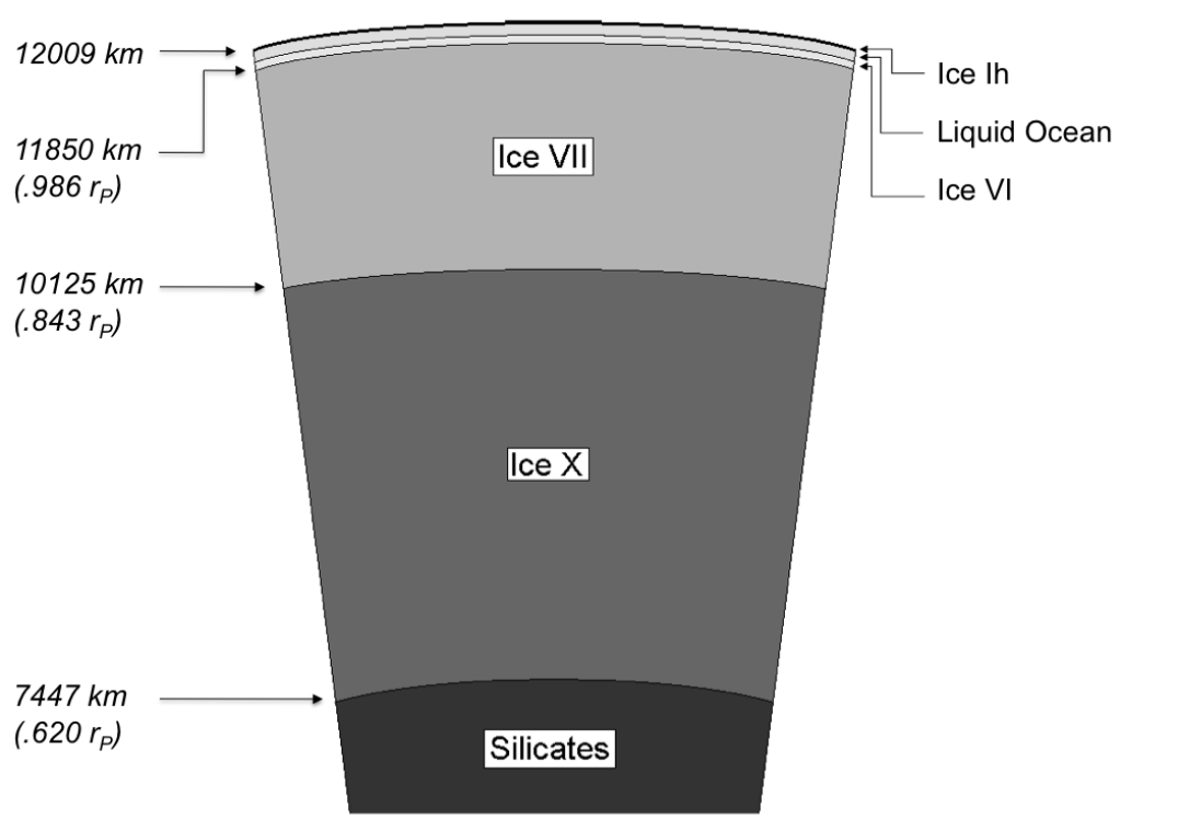
Figure 1: The $H_{2}O$ region of the $5\,M_{Earth}$, $50\%\,H_{2}O$ planet drawn to scale. This configuration estimates heat flux according to Equation 2.

A scaled diagram of the $H_{2}O$ region of our $5\,M_{Earth}$, $50\%\,H_{2}O$ planet is shown in Figure 1. Note that the details in the Ice VI, liquid water, and Ice Ih layers were found after the thermal modeling in the subsequent sections.

3 Thermal Models

We include two sets of thermal models. The first models the near-surface region of the planet, both in the case of a frozen surface and a liquid surface. The second models convection in the underlying mantle of higher-phase ices.

3.1 Near surface convection

We consider the case where the surface temperature is below the freezing point. We model both conductive and convective heat flow in the near-surface region. We define the superficial ice layer where heat transport is solely due to conduction as the “crust.” For the thickness of the crust, we use the simple expression for a conductive thermal profile:

$$D=\frac{k(T_{B}-T_{S})}{q_{S}}$$ (1)

Where $D$ is the thickness of the crust, $T_{B}$ and $T_{S}$ are the temperatures at the base and at the surface, $q_{S}$ is the surface heat flux, and $k$ is the thermal conductivity of Ice Ih, equal to $3.3\,Wm^{-1}K^{-1}$ (Spohn and Schubert, 2003). $T_{S}$ and $q_{S}$ are left as the independent variables in this analysis. The former is determined by the planet’s insolation, albedo, and atmospheric effects, while heat flux can be estimated by scaling the planetary heat output with the total mass of silicates and metals ($M_{eff}$) compared to the Earth, and then adjusting this quantity to the desired radius ($r$):

$$q_{s}=q_{Earth}\frac{M_{eff}}{M_{Earth}}(\frac{r}{r_{Earth}})^{-2}$$ (2)

Where $q_{Earth}=0.087\,W/m^{2}$ (Turcotte and Schubert, 2002). This estimate for heat flux is only used in this work for analyzing the convection of the ice mantle (Section 3.2).

We evaluate the convective stability of the surface ice layer by finding its Rayleigh number ($Ra$) and comparing it to a critical Rayleigh number ($Ra_{crit}$). The former is given by:

$$Ra=\frac{g\alpha\rho D^{3}(T_{B}-T_{S})}{\kappa\eta(T_{B},T_{S})}$$ (3)

Where $g$ is the surface gravity, $\alpha=1.6\times 10^{-4}\,K^{-1}$ is the thermal expansivity of Ice Ih, $\rho=917\,kg\,m^{-3}$ is its density, and $\kappa=3.7\times 10^{-6}\,m^{2}s^{-1}$ is its thermal diffusivity (Spohn and Schubert, 2003). The viscosity $\eta$ is strongly temperature dependent. Given the low pressure regime found in the crust, we assume a Newtonian, volume diffusion-dominated rheology following the work of Mueller and McKinnon (1988):

$$\eta(T)=\eta_{0}\exp[\frac{Q^{*}}{RT_{\eta}}]$$ (4)

We adopt values of $139$ $Pa\cdot s$ and $56.7$ $kJ/mol$ for $\eta_{0}$ and $Q^{*}$, respectively, corresponding to a grain size of $\approx 0.2\,mm$ for our temperature range (McKinnon, 2006).

We note that the stability of the conductive boundary layer has been used to derive the relation $Nu=A\cdot Ra^{\beta}$, where $Nu$ is the Nusselt number and $A$ and $\beta$ are constants. Scaling relations of this form are used to relate the convective heat flux to the parameters governing convection (Howard, 1966), and they yield the same result as more complete boundary layer models (O’Connell and Hager, 1980; Turcotte and Schubert, 2002; Valencia and O’Connell, 2009). Where applicable (i.e. in the case of convection in an Ice Ih shell overlying a liquid ocean), this scaling has been verified to corroborate our results.

We evaluate Equations 1, 3 and 4 under two distinct formulations. For relatively high $T_{S}$ ($\gtrsim 190\,-\,220\,K$, depending on curve being calculated), we find that the viscosity contrast is relatively small ($\mbox{$\eta$}_{max}/\eta_{min}\lesssim 10^{3}$). We therefore employ the small viscosity contrast (SVC) presciption, with characteristic viscosity taken to be the value corresponding to the average temperature: $T_{\eta,\,SVC}=(T_{B}+T_{S})/2$. This approximation has been found to be appropriate for viscosity contrasts of up to $\eta_{max}/\eta_{min}\approx 10^{4}$ (Dumoulin et al., 1999). In this regime, we use a critical Rayleigh number of $Ra_{crit,\,SVC}=2000$, corresponding to viscosity contrasts of $10^{3}$ (Schubert et al., 2001).

For relatively low $T_{S}$ and correspondingly high viscosity contrasts, we use the stagnant-lid formulation to describe convection. In this case, convection is limited to an adiabatic zone in the lowest part of the ice layer. The characteristic viscosity of the convection cell is found by evaluating Equation 4 with the temperature at the bottom of the conductive crust: $T_{\eta,\,SL}=T_{B}$ (Solomatov, 1995). The corresponding critical Rayleigh number is dependent on the magnitude of the viscosity contrast: $Ra_{crit,\,SL}=20.9p^{4}$ where $p$ reflects the logarithm of the viscosity contrast between the top and bottom of the full ice layer (Solomatov and Moresi, 2000):

$$p=\frac{Q^{*}}{R}(\frac{T_{B}-T_{S}}{T_{i}^{2}})$$ (5)

Where $T_{i}$ is the temperature in the actively convecting region. It is cooler than $T_{B}$ by a small amount on the order of $10\,K$: ($T_{B}-T_{i}\approx RT_{i}^{2}/Q^{*}$).

Using the appropriate formulation for the given viscosity contrast, we solve for the maximum thickness of the conductive crust and the bottom temperature $T_{B}$ as functions of the imposed parameters $q_{S}$, $T_{S}$, and $g$. If this maximum conductive thickness is greater than that of the Ice Ih layer before it meets the melting curve, then our crust directly overlies a liquid ocean, which has an adiabatic temperature profile. Otherwise, we find solid-state convection immediately below the crust.

In the case of a liquid surface, we model the temperature gradient in the surface ocean to be adiabatic. The thickness of this ocean is found by identifying the intersection of this adiabat with the freezing curve of water at depth.

3.2 The ice mantle

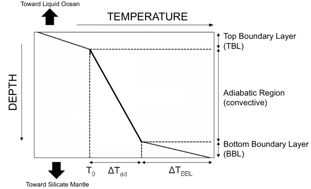
Figure 2: The qualitative features of the thermal profile within the ice mantle. The temperature in the TBL is bound to the melting curve while that of the BBL is conductive.

Regardless of the near-surface structure, convection is always present in the underlying layers of higher phase ices (henceforth called the “ice mantle”). We assume for now and show below that convection within the ice mantle is not partitioned by phase transitions. We also assume a rectangular geometry for the convective layer, a valid approximation given that the analysis focuses on only the boundary layers. For the case where the ice mantle underlies a liquid ocean, we adopt a thermal profile as shown in Figure 2. This thermal profile is partitioned into an adiabatic region between two boundary layers. The Bottom Boundary Layer (BBL) is a conductive zone that corresponds to the thin region where the cold material recently arrived from above is slowly heated by conduction from the underlying silicates until it rises again.

On the other hand, the temperature profile in the top boundary layer (TBL) is constrained to follow the melt curve. The dynamical characteristic of this region is outlined further in the discussion (Section 5). The top interface temperature $T_{T}$ and depth $z_{T}$ correspond to the temperature and location of the bottom of the liquid ocean and are constrained by the above considerations of the near-surface thermal profile. To constrain the quantities $T_{0}$, $\Delta T_{ad}$, and $\Delta T_{BBL}$ (see Figure 2), we construct a convection model that uses three independent relations: one governing each boundary layer and one describing the adiabat. We note that we do not explicitly use any existing Nusselt - Rayleigh number scaling laws. However, our model considers precisely the same physics that forms the basis of such scaling laws- namely by assuming that both boundary layers are at the verge of convective stability (see Valencia and O’Connell, 2009, the Appendix for a detailed derivation).

First, we examine the convective stability of the TBL. In all six of our examined ice mantles (of the $25\%$ and $50\%$ $H_{2}O$ planets), when approximating heat flux by Equation 2, the TBL is composed entirely of Ice VI. The thickness ($\delta_{TBL}$) and bottom temperature ($T_{0}$) in the TBL is therefore related simply by following the melt curve of Ice VI:

$$\delta_{TBL}=\frac{T_{0}-T_{VI}}{m_{VI}}-z_{T}$$ (6)

Where $T_{VI}$ and $m_{VI}$ are the $T$-intercept and slope of the Ice VI melt curve, respectively, and $z_{T}$ is the depth of the bottom of the liquid ocean. The Rayleigh number of the TBL can then be calculated and set equal to the critical Rayleigh Number ($Ra_{crit}$), chosen to be $1000$ to reflect the mild viscosity contrast within the layer (Turcotte and Schubert, 2002):

$$Ra_{TBL}=Ra_{crit}=\frac{g\alpha\rho(T_{0}-T_{T})\delta_{TBL}^{3}}{\kappa\eta_{TBL}}$$ (7)

Where $\eta_{TBL}$ is the viscosity in TBL evaluated for the average temperature and pressure, as appropriate for smaller viscosity contrast (McKinnon, 1998). $T_{0}$ may be obtained from Equations 6 and 7, allowing for the evaluation of the adiabatic temperature gradient via the following relationship (Turcotte and Schubert, 2002):

$$\frac{dT(z)}{dz}\approx\frac{T(z)\,g\alpha(P(z),\,T(z))}{C_{p}(T(z))}$$ (8)

Where $C_{P}(T)$ is the isobaric specific heat capacity. Equation 8 can be integrated numerically from bottom of the TBL to the top of the BBL to find the temperature change in the adiabatic regime $\Delta T_{ad}$ as a function of $T_{0}$.

Finally, we evaluate the Rayleigh number of the BBL and set it to the critical Rayleigh number $Ra_{crit}$, again chosen to be $1000$. Defining $\delta_{BBL}$ to be the thickness of the BBL, we can write the Rayleigh number and the heat flux as:

$$Ra_{BBL}=Ra_{crit}=\frac{g\alpha\rho\Delta T_{BBL}\delta_{BBL}^{3}}{\kappa\eta_{BBL}}$$ (9)

$$\delta_{BBL}=\frac{k\Delta T_{BBL}}{q_{BBL}}$$ (10)

Where $\eta_{BBL}$ is the BBL viscosity, which is dependent on the value of $T_{0}$ and $T_{ad}$, and is once again calculated for small internal viscosity contrast. Combining Equations 9 and 10 allows the calculation of the final unknown, $\Delta T_{BBL}$.

Due to the much higher pressure and temperatures in the ice mantle, the assumptions of Newtonian rheology and constant $\alpha$ as in our near-surface analysis are insufficient. Under the stress regime in our ice mantles (several $MPa$, see below), dislocation creep, which has a significant stress dependence, is expected to dominate (Durham and Stern, 2001). Furthermore, the viscosity change between known ice phases under this stress regime is not great ($<10^{2}$). Hence, we use a dislocation creep model for the viscosity of Ice VI, the highest pressure phase measured to date, for the ice mantle (Durham et al., 1997):

$$\eta(P,\,T)=6.65\times 10^{19}\,\sigma^{-3.5}\,\exp[-(E^{*}+PV^{*})/RT]$$ (11)

Where $\sigma$ is a characteristic shear stress, $R$ is the ideal gas constant, and $E^{*}$ and $V^{*}$ are the activation energy and volume, measured to be $110\,kJ/mol$ and $1.1\times 10^{-5}\,m^{3}/mol$, respectively. Owing to the lower viscosity of ice compared to silicates, the shear stress is approximated to be a value somewhat lower than that of the Earth’s mantle, $2\times 10^{6}\,Pa$. This value is self-consistent with our results. The activation volume $V^{*}$ itself changes with depth; it can be approximated to shrink with pressure as a vacancy in the material. Following the analysis of O’Connell (1977), the effective bulk modulus of this vacancy is:

$$K^{*}=V^{*}\frac{\partial P}{\partial V^{*}}=\frac{2(1-2\nu)}{3(1-\nu)}K$$ (12)

Where $K$ is the bulk modulus of the material and $\nu=0.35$ is the Poisson ratio. By expanding $K$ to first order in pressure and integrating Equation 12, we obtain the activation volume as a function of pressure:

$$V^{*}(P)=V_{0}^{*}(\frac{K_{0}^{*}+K^{\prime*}P}{K_{0}^{*}+K^{\prime*}P_{0}})^{-\frac{1}{K^{\prime*}}}$$ (13)

Combining Equations 11 and 13 gives viscosity as a function of depth for a specified thermal profile. Under this formulation for viscosity, our results show that maximum viscosity contrasts in the TBL are on the order of $10^{2}$, while that of the BBL are similar in most cases, except for the $2\,M_{Earth}$ planets, where the contrasts are between $10^{5}$ and $10^{7}$. Despite this, we maintain the use of the small viscosity contrast formulation for BBL viscosity due to (1) the fact that varying $\eta_{BBL}$ through its entire possible range does not change our ultimate results (overturn timescale, etc) by more than a factor of a few and (2) the lack of existing theory for bottom boundary layers with high viscosity contrast. Note that the viscosity contrasts within the TBL are much smaller than values for the icy crust due to the viscosity-reducing effects of pressure and the shallower thermal gradient due to the melting curve.

As for the depth-dependent parameters $\alpha(P,\,T)$ and $C_{P}(T)$, we use results obtained for Ice VII. Fei et al. (1993) have produced the following expression for $\alpha(P,\,T)$ , in units of $K^{-1}$:

$$\alpha(P,\,T)=(3.9\times 10^{-4}+1.5\times 10^{-6}T)(1+\frac{K^{\prime}_{0T}}{K_{0T}}P)^{-0.9}$$ (14)

We again use the results from Fei et al. (1993) to obtain $C_{P}$ in units of $J\,kg^{-1}\,K^{-1}$:

$$C_{p}(P,\,T)=4027.22+0.168T-8.011\times 10^{7}\frac{1}{T^{2}}$$ (15)

Finally, we test throughgoing convection at phase transitions throughout the ice mantle. A sufficiently endothermic phase transition (i.e. the Clapeyron slope, $\gamma$, is sufficiently negative) can partition convection by introducing temperature-driven topography to the phase boundary. We evaluate the dimensionless “phase buoyancy parameter” ($P_{b}$) for all endothermic transitions, given by (Christensen and Yuen, 1985):

$$P_{b}\equiv\bar{\gamma}\frac{Rb}{Ra}=\gamma\frac{\Delta\rho}{\bar{\rho}^{2}gh\alpha}$$ (16)

Where $Rb$ is the boundary Rayleigh number which uses a phase-driven instead of thermal-driven density contrast, $\gamma$ is the Clapeyron slope, $\Delta\rho$ is the density contrast across the transition, $\bar{\rho}$ is the mean density, and $h$ is the full thickness of the unpartitioned convective layer. Our values for $\Delta\rho$ are calculated from EOSs for the relevant ice phases, while $\gamma$ was obtained directly from the literature or calculated with published triple point data. See Table 4 for a listing of relevant references.

4 Results

We obtain mass-radius relationships for water planets from our hydrostatic models. Following the work of Valencia et al. (2007b), we fit our results to a function of total mass of the form:

$$\frac{r_{P}}{r_{Earth}}=A(\frac{M_{P}}{M_{Earth}})^{B}$$ (17)

With values for $A$ and $B$ given for a range of water compositions in Table 2. The silicate - metal ratio in each case is $2.09$. We find that Ice X lies at the bottom of the $H_{2}O$ shell of the $25\%$ and $50\%$ $H_{2}O$ planets except for the $2\,M_{Earth}$, $25\%\,H_{2}O$ case (see Table 3). In the cases of Earth-like water mass fraction, we find either Ice Ih or liquid water at the $H_{2}O$ - silicate boundary, depending on the near-surface temperature profile (see below).

For the planets with ice phase transitions ($25\%$ and $50\%\,H_{2}O$ planets), our analysis of convective breakthrough revealed no phase transitions that should partition convection. As an example, the relevant parameters and $P_{b}$ values for the $5\,M_{Earth}$, $50\%\,H_{2}O$ exoplanet ($h\approx 4400\,km$) are listed in Table 4. Note that our predictions of convective breakthrough at the Ice Ih - III and Ice II - V boundaries diverge from the corresponding results for the icy satellites (McKinnon, 1998). This is due to the much greater thickness $h$ of the convective cell in our exoplanet. For a much smaller exoplanet closer to the Galilean satellite instead of super-Earth regime, given an ice mantle thickness on the order of a few hundred $km$, these two transitions may hinder convection.

Our models of the frozen surface case reveal that four qualitatively distinct dynamical Regimes exist for the near-surface region. For a given rheology, the Regimes are determined by the surface temperature $T_{S}$, heat flux $q_{S}$, and, to a lesser extent, gravity $g$. The parameter space in which one finds each of the four layering regimes is shown for the $g=15\,m/s^{2}$ and $g=10\,m/s^{2}$ cases in Figure 3. A liquid ocean is present for Regimes I and II. In Regime I, the Ice Ih layer overlies a liquid water ocean and is not of sufficient thickness to convect. In Regime II, the temperature profile still intersects the melting curve within the Ice Ih region, thus maintaining the presence of an ocean. However, the Ice Ih region in this case is convectively unstable, and some solid-state convection is found at the base of this region. The boundary between Regime I and Regime II is calculated by setting the Rayleigh number of the strictly Ice Ih region above the ocean layer to the critical Rayleigh number ($Ra_{crit}$): if the Rayleigh number is above $Ra_{crit}$, the planet is in Regime II. The kink in this curve at $\approx 225\,K$ is due to a transition between the usage of stagnant-lid formulation for lower $T_{S}$ and small viscosity contrast formulation for higher values. At lower $T_{S}$ values, increasing the temperature lowers the viscosity and expands the parameter space where convection occurs. However, as $T_{S}$ continues to increase, eventually the thinning of the crust inhibits convection, hence the characteristic “humped” shape of the Regime I - II boundary.

In Regime III, the “turn off point” in the temperature profile- the point at which the switch is made from conductive to convective heat transfer- is below the minimum temperature of the melting curve ($251\,K$). Therefore, we find no liquid ocean. Instead, given the penetration of the Ice Ih - III and Ice Ih - II interfaces, we find a convection cell immediately below the crust that extends down to the silicate - ice boundary. Finally, in Regime IV, a thick, convectively stable crust extends below the region occupied by Ice Ih and meets the melting curve before the onset of convection. The temperature profile, when it reaches the melting temperature, is bounded by the melting curve. This must be the case: the temperature cannot be higher than the melting curve since the liquid would rapidly carry away heat, refreezing the material. The temperature profile must therefore follow the melting curve until this transition layer becomes convectively unstable, at which point it dives to greater depths along an adiabat. The dynamical properties of this region bound to the melt curve are considered further below under Discussion.

The curve separating Regime III from Regimes II and IV is the contour for a constant “turn off point” temperature of $251\,K$. Meanwhile, the line separating Regimes I and IV corresponds to the scenario where the conductive portion of the temperature profile intersects the melt curve at the Liquid - Ice Ih - Ice III triple point: $T=251\,K$ and $P=210\,MPa$. If the intersection with the melt curve occurs at lower pressure (above the Regime I - IV boundary in Figure 3), the temperature profile intersects the melting curve within the Ice Ih domain and therefore falls into Regime I.

Our formulation for Newtonian viscosity (Equation 4) is subject to uncertainty due to the unknown characteristic grain size in the Ice Ih crust of exoplanets. Compared to the $\approx 0.2\,mm$ we used in our analysis, Galileo observations of Europa has produced estimates of $0.1\,mm$ for surficial grain size and estimates of several millimeters in the underlying regions (Pappalardo et al, 1998). Assuming that volume diffusion continues to be the dominant creep mechanism, increasing the grain size to $0.5\,mm$ increases the constant $\eta_{0}$ in Equation 4 by a factor of six ($\eta\propto d^{2}$) and lowers the required $q_{S}$ value for all Regime boundaries by about a factor of two, although their $T_{S}$ coordinate remains essentially identical (see Figure 3). The uncertainty in grain size, and hence Ice Ih viscosity, is the single greatest uncertainty in our analysis of the ice crust, and care should be taken to consider a range of possible grain sizes when attempting to characterize the surface of a specific water planet.

A further source of uncertainty lies in the possibility of the presence of solutes or other volatiles in significant quantities within the ocean layer, thereby depressing the freezing point of the water-solute mixture, resulting in thinner and colder crusts, possibly hindering convection. We test the case of a water-ammonia mixture by adopting the phase diagram of the $H_{2}O$ - $NH_{3}$ system as proposed by Hogenboom (1997). Assuming $NH_{3}$ concentration of $10\%$, we find a modest correction to the Regime I - II boundary curve (see Figure 3).

As pointed out by the referee, we ignore the transition regime between the low viscosity contrast and stagnant-lid convection regimes. Given that our calculations yield Rayleigh numbers on the order of $10^{5}$ to $10^{6}$ for the Ice Ih shell in Regime II and $>10^{6}$ for Regimes III and IV (equal to $Ra$ of the full ice mantle convection in these latter cases), the surface temperature range over which the transitional regime is valid is between $T_{S}\approx 190\,K$ and $235\,K$. As the plausible deviation from our interpolation inside this narrow range is small compared to the magnitude of the other uncertainties that exist, we accept our current results as sufficiently accurate while noting that fuller consideration of the transitional regime may be worthwhile in a future work.

Although it is not plotted in Figure 3, we imagine a separate regime where $T_{S}$ is above freezing, resulting in a liquid ocean at the surface. The temperature profile in such an ocean is adiabatic until it freezes into higher phase ices at a depth on the order of $10$s to a few $100$s of $km$.

We apply our convection model for the ice mantle underlying a liquid ocean to the $25\%$ and $50\%\,H_{2}O$ exoplanets with $T_{S}=250\,K$. The near surface structure is first determined in each case, yielding the result the crust in all these cases fall into Regime I. As an example, in the $5\,M_{Earth}$, $50\%\,H_{2}O$ case we find that an ocean of $62\,km$ thickness underlies a brittle crust only $1.2\,km$ thick. The ocean bottom temperature is $T_{T}=283\,K$; this figure is virtually constant for all six cases to within two degrees. The full solution to the temperature profile in the ice mantle for selected exoplanets is shown in Figure 4. We find that due to the smaller adiabatic temperature change and the correspondingly lower temperature at the top of the BBL, $\Delta T_{BBL}$ is significantly larger for planets with the smallest $H_{2}O$ shells.

We can estimate the full ice mantle Rayleigh number of each planet. As described further in the Discussion section, finding a characteristic viscosity for the ice mantle is elusive due to its complex depth-dependence, reaching a viscosity maximum in mid-layer. We employ a simple approximation by taking the logarithmic average of the the viscosity throughout the ice mantle. This estimate results in Rayleigh numbers for the ice mantle between $10^{5}$ and $10^{9}$, with the smallest Rayleigh numbers corresponding to the for the least massive planets with the thinnest water shell.

The overturn time of the ice mantle (i.e. time needed for material from the silicate - ice boundary to reach the top of the ice mantle) can now be calculated. Turcotte and Schubert (2002) have found by theoretical considerations that, given a cell aspect ratio of unity, the maximum velocity of convective material should depend on the full mantle Rayleigh number $Ra_{m}$:

$$u_{0}=0.271\frac{\kappa}{h}Ra_{m}^{2/3}$$ (18)

The overturn time scale is then simply calculated by dividing the thickness of the ice mantle by $u_{0}$. The results of this calculation for a range of planetary masses and water mass fractions, as well as their uncertainties, are shown in Table 5. A word about the associated errors is found in Discussion.

5 Discussion

If a water planet has a frozen surface, the Regime of the crust has direct impact on observable features. In Regimes I and II, the presence of a liquid ocean layer is expected to bias the set of outgassed compounds towards species that are water-transportable, since, although solid-state convection through the mantle of higher ice phases can dredge up material expelled from the silicate - metal core, predominantly materials that can be dissolved or suspended in liquid water are able to traverse the ocean layer. A more detailed, quantitative analysis of this selection process is left for future work.

In Regimes II, III, and IV, the presence of solid-state convection immediately below the brittle crust may lead to the existence of ice tectonics. This provides a means by which the chemistry of the convection cells can continuously gain a window to the surface, altering the atmospheric observables of the exoplanet (Valencia et al., 2007c). A simple test for the presence of ice tectonics is to compare the tensile strength of Ice Ih as found on the surfaces of icy satellites ($\approx 1\,MPa$, Nimmo and Schenk 2006) and the expected tensile stress imposed on the crust by the convection cell. The approximate stress imposed by underlying convection is (McKinnon, 1998):

$$\sigma_{conv}\approx\frac{g\alpha\rho h\Delta T_{\sigma}}{3Ra_{crit}^{1/3}}$$ (19)

Where again $h$ and $\Delta T_{\sigma}$ are the height and driving temperature contrast of the convective region, respectively. The tensile stress on the brittle crust may then be amplified if the thickness of the crust $D$ is smaller than the horizontal length over which a convection cell is in contact with the crust. Assuming a convection cell aspect ratio of unity, the stress on the crust is therefore $\tau=\sigma_{conv}h/D$.

Performing this analysis for a crust in Regime II, we find that even in the case of small $D$ ($3\,km$) and high $\Delta T_{\sigma}$ ($40\,K$), $\tau$ does not rise beyond $220\,kPa$ for $g$ between 10 and $20\,m/s^{2}$. Therefore, the crust in Regime II is probably not directly broken apart by stresses due to solid-state convection alone. However, resurfacing may persist in Regime II and even Regime I crusts due to a range of other phenomena that have been observed on the large icy satellites of the solar system. Such surface processes include diapirism (Europa- Pappalardo et al, 1998; Triton- Schenk and Jackson, 1993), cryovolcanism (Titan- Lopes et al, 2007), and planetary-scale tectonics (Ganymede- Head et al, 2002; Europa- Showman and Malhotra, 1999), although the last of these maybe require exogenic sources of stress such as tidal forces in addition to internal processes. The presence of solid-state convection is found to facilitate these forms of resurfacing (e.g. diapirism- Pappalardo et al, 1998; cryovolcanism-Mitri et al., 2008), although penetration of the icy crust by underlying fluids may still be possible in the absence of convection (Showman et al, 2004). Alternatively, a Regime II crust may be completely devoid of surface activity as in the case of Callisto (Showman and Malhotra, 1999).

As considerations of these solar system bodies show, reliably constraining the outgassing into the atmospheres of Regimes I and II planets is not possible given only the dynamical and thermal structure of the ice shell, as presented in this paper.

On the other hand, in Regimes III and IV, the stress on the lithosphere is greatly increased for two reasons. First, because the convection cells extend to the base of the $H_{2}O$ layer of the planet, $\sigma_{conv}$ is much larger due to greater values for $h$ and $\Delta T_{\sigma}$. Second, assuming convective cells with aspect ratios of near unity, the amplification from the $h/D$ factor is much greater. We find that in the $25\%$ and $50\%$ water cases considered in this work, the crust is easily broken by convection-driven stresses ($\tau\approx 10^{3}\,MPa$ for a thick, $50\,km$ crust), leading to continuous global resurfacing under these Regimes. This result is consistent with analogous analysis for super-Earths with rocky surfaces; as shown in Valencia and O’Connell (2009), the higher convective stresses in the mantles of large silicate planets likewise outcompetes the tensile strength of the brittle crust.

Finally, in the liquid surface case, chemical species released into the atmosphere should again be selected for water-transportable types, but outgassing on the surface proceeds unhindered. In this respect, the properties of outgassed material may be similar to those of Regimes I and II, while the flux may be similar to that of Regimes III and IV.

Several uncertainties exist for our model of convection in the ice mantle. The true viscosity of the Ice VII and Ice X is unconstrained, as ice viscosity has not been measured at pressures of greater than about $0.8\,GPa$. The viscosity deep in the ice mantle is determined by the balance between three processes: increasing pressure, which increases the activation energy; shrinking activation volume, which tempers the above effect of pressure; and increasing temperature. Interestingly, all resulting mantle thermal profiles show a viscosity maximum in mid-layer of the ice mantle with viscosity values between $10^{21}$ and $10^{23}\,Pa\cdot s$. This is due to the initial dominance of the pressure effect over the adiabatic temperature increase owing to a relatively large activitation volume. However, as the vacancies of the material become increasingly compressed at depth, the viscosity decreases with increasing temperature. This effect leads to low BBL viscosities of as little as $10^{14}\,Pa\cdot s$ for the $10\,M_{Earth}$, $50\%\,H_{2}O$ planet. Such results may not reflect true values and improved results must await the availability of additional rheological data for high-pressure ices. Furthermore, more refined results call for new theory that characterizes convection with a viscosity maximum in mid-layer and provides for a means to determine a characteristic viscosity.

Values for certain other parameters in the mantle Rayleigh number, such as $g$ and $\alpha$ are difficult to choose to be representative of the ice mantle. We find that varying these throughout their possible range generally leads to a change of a factor of a few in the resulting overturn time. Combined with the greater uncertainty resulting from the characterization of viscosity as described above, the results in Table 5 are presented as estimates to within around one order of magnitude instead of precise solutions. We note, however, that despite these uncertainties, the qualitative phenomenon of a mid-layer high viscosity region is relatively certain, as the effect is apparent even when varying the parameters in the viscosity law beyond the range of published values (Durham et al., 1997).

A further point of ambiguity is whether the steep rise in temperature along the adiabat in the lower parts of the ice mantle will cause our thermal profile to intersect the melting curve again at depth. Recent studies of the melting curve of high pressure ice phases suggest that this may occur only for a planet with a much larger water layer. Schwager et al. (2004) found experimentally that at $100\,GPa$ corresponding to a the melting point of the Ice X is 2400 K, while our ice mantle temperatures are confined to under $1200\,K$ (Figure 4).

A word must be said about the behavior of material where the temperature is constrained to the melting curve. This situation arises at the top of the ice mantle when the crust falls into Regimes I, II, or IV. In Regimes I and II, a liquid ocean overlies the ice mantle, and the temperature profile runs along the melt curve until convective instability is reached in this boundary layer.

Although the globally averaged temperature proceeds along the melt curve in these cases, the full 3-D scenario is more complicated. Qualitatively, we expect the upward heat flux in this transition zone to be carried by the percolation of liquid water in certain concentrated zones. We describe a feedback mechanism that leads to the creation of narrow zones of rising meltwater. Beginning with a laterally homogeneous transition layer, if a packet of material should melt in a specific location, say due to the presence of an underlying hot plume, this packet of material immediately undergoes a decrease in density, which leads to a decrease in the pressure in the underlying column. A decrease in pressure leads to the melting of ice previously at equilibrium, further promoting the creation of meltwater in the column. More detailed considerations of this process should be performed in the future.

6 Conclusions

In this work we have modeled the interior dynamics of the $H_{2}O$ layer of water planets. We first study the thermal and dynamical properties of an ice crust for a planet with sub-freezing $T_{S}$. We find that the dynamical behavior of the crust falls into one of four Regimes (Figure 3), primarily determined by the planetary parameters surface temperature and heat flux, with a weaker dependence on surface gravity. Planets with a crust in Regimes III and IV should show atmospheric signatures of close to the full range of possible compounds produced from materials released from the silicate - metal core. Ice tectonics under these Regimes is expected to bring about continual resurfacing. The atmosphere of Regimes I and II planets may or may not be enriched by outgassing, depending on the presence of resurfacing phenomena such as cryovolcanism and other sources of stress (e.g. tides). As evidenced by the examples of such bodies studied in our solar system, the surface geology of icy bodies in these Regimes is difficult to constrain without case-specific considerations of a wider range of resurfacing processes.

In the case of Regimes I and II, the range of materials that is able to reach the surface is affected by the presence of a liquid ocean layer, which selects for materials that can exist in solution or suspension. A more detailed study of this process is important for work future work. In the case of a liquid surface layer, we expect a full flux of outgassed materials biased by its transportability through the liquid ocean.

Our model of the ice mantle composed of higher-phase ices shows that materials expelled from the silicate - metal core into the ice layer can traverse the ice mantle on the time scale of $0.1$ to a hundred $Myr$ for the cases examined with shorter overturn times corresponding to larger planets. New constraints on the rheology of higher-phase ices as well as theory to describe the behavior of convection with a mid-layer viscosity maximum are required to obtain more accurate results. The specific chemical composition and mass flux of such dredged and outgassed material should be investigated quantitatively in further studies, ultimately leading to specific predictions of the atmospheric detectables of water planets.

7 Acknowledgements

We thank Diana Valencia, Lisa Kaltenegger and Wade Hennings for discussions that led to advances in understanding and the conception of the scope of this paper. This work is supported by the Harvard University Origins of Life Initiative.

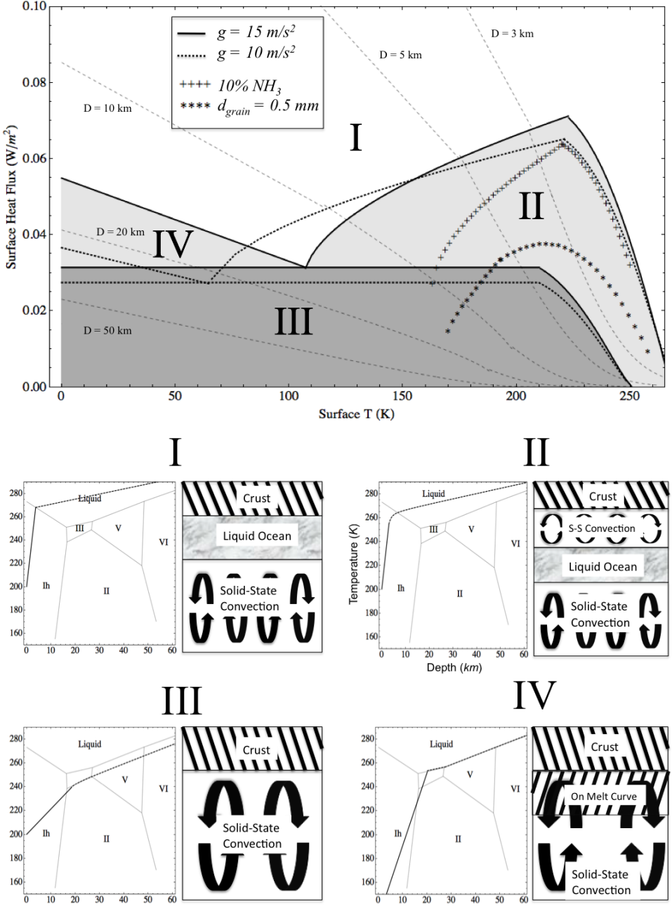
Figure 3: The four Regimes of the crust as a function of $T_{S}$ and $q_{S}$ for the $g=15\,m/s^{2}$ and $10\,m/s^{2}$ cases. Contours of constant crustal thickness for $g=15\,m/s^{2}$ are plotted as light dashed lines in the top diagram. See Section 4 for explanation of the boundaries of each regime. Depth scale in the phase diagrams are based on the $5M_{Earth}$, $50\%\,H_{2}O$ planet. The cartoon cross-sections are not drawn to scale. In the liquid surface case, the cross-section would appear as in Regime I, only without the “Crust” section; its thermal profile would begin at an above-freezing temperature at the surface and be adiabatic throughout the liquid ocean.

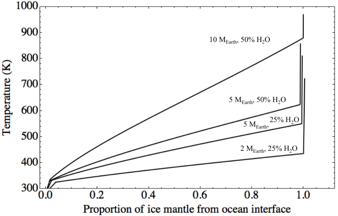
Figure 4: Complete temperature profile of the ice mantle of four selected water planets plotted against normalized depth from the ocean - Ice VI contact. True mantle thicknesses are: $1910\,km$, $2460\,km$, $4500\,km$, and $5425\,km$ for the four planets plotted in ascending order as seen in the figure (i.e. $1910\,km$ corresponds to the $2\,M_{Earth}$, $25\%\,H_{2}O$ planet, etc). The locations of the bottom boundary layers have been staggered in order to show the magnitude of temperature change.

Component	EOS	$\rho_{0}\,(\frac{kg}{m^{3}})$	$K_{0T}\,(GPa)$	$K^{\prime}_{0T}$	$K^{\prime\prime}_{0T}\,(GPa^{-1})$	Ref.
$Fe$	Vinet	8300	156.2	6.08	-	1
$MgSiO_{3}$	B-M 4	4100	247	3.97	-0.016	2
$Ice\,X$	B-M 3	1239	4.26	7.75	-	3
$Ice\,VII$	B-M 3	1463	23.7	4.15	-	4
$Ice\,Ih$	B-M 3	917	9.86	6.6	-	5, 6

Table 1: Equations of state and elastic parameters used in calculation of static planetary dimensions. B-M 3 and B-M 4 refers to the 3rd and 4th order Birch-Murnaghan equations of state while $\rho_{0}$ and $K_{0T}^{n}$ are the zero-pressure density and pressure derivatives of the isothermal bulk modulus, repectively.

References: (1) Anderson et al, 2001 (2) Karki and Wentzcovitch, 2000 (3) Loubeyre et al., 1999 (4) Hemley et al, 1987 (5) CRC Handbook, 1969 (6) Strassle et al., 2005

Constant	$0.02\%\,H_{2}O$	$25\%\,H_{2}O$	$50\%\,H_{2}O$
$A$	$0.994$	$1.157$	$1.255$
$B$	$0.266$	$0.253$	$0.251$

Table 2: Constants for the mass-radius scaling relation (Equation 17).

$H_{2}O$ Content	$2\,M_{Earth}$	$5\,M_{Earth}$	$10\,M_{Earth}$
$25\%\,H_{2}O$	$47.8\pm 1.0\,GPa$	$115.3\pm 1.6\,GPa$	$236.6\pm 2.6\,GPa$
$50\%\,H_{2}O$	$86.2\pm 2.0\,GPa$	$212.0\pm 2.2\,GPa$	$436.9\pm 3.6\,GPa$

Table 3: Pressures at the ice - silicate boundary. Values greater than about $60\,GPa$ indicate the prescence of Ice X. Errors are determined by using the extremes of each equation of state parameter that yields the lowest and highest pressure.

Transition	$\Delta\rho\,(kg/m^{3})$	$\gamma\,(MPa\,K^{-1})$	$P_{b}$	Ref. for $\Delta\rho$	Ref. for $\gamma$
$Ih-III$	$218$	$-0.47$ - $-0.24$	$-0.01$ - $-5\times 10^{-3}$	1	2; 3
$II-V$	$38$	$-8.9$ - $-0.67$	$-0.025$ - $-.002$	1, 4	2; 3, 5
$II-VI$	$48$	$\approx-1.7$	$\approx-5\times 10^{-3}$	1, 4	6
$VII-X$	$68.1$	$-11$ - $+26.3$	$-0.01$ - $+0.02$	7, 8	9; 10

Table 4: The phase buoyancy parameter $P_{b}$ for all encountered endothermic phase transitions between the water ices. Throughgoing convection is unhindered if $P_{b}\gtrsim-0.3$. Since the Clapeyron slope $\gamma$ is the most uncertain parameter in $P_{b}$ (see Equation 16), the range of values of $P_{b}$ is found by evaluation with a range of $\gamma$ values found in the literature.

References: (1) Shaw, 1986 (2) McKinnon, 1998 (3) Bridgman, 1912 (4) Leon et al., 2002 (5) Mercury et al., 2001 (6) Durham et al., 1997 (7) Loubeyre et al., 1999 (8) Hemley et al, 1987 (9) Song et al., 2003 (10) Goncharov et al., 1999

$H_{2}O$ Content	$2\,M_{Earth}$	$5\,M_{Earth}$	$10\,M_{Earth}$
$25\%\,H_{2}O$	$83\,Myr$	$16\,Myr$	$0.8\,Myr$
$50\%\,H_{2}O$	$190\,Myr$	$12\,Myr$	$0.3\,Myr$

Table 5: Order of magnitude estimates for the overturn time scale for the ice mantles. Numbers represent the time for material to rise from ice - silicate boundary to the top of the ice mantle. The values for the $10\,M_{Earth}$ planets are not as well-constrained. See the Discussion section for further notes about uncertainties.

References

- Anderson et al (2001) Anderson, O. L., Dubrovinsky, L., Saxena, S. K., & LeBihan, T. 2001, Geophys. Res. Lett., 28, 399
- Barr and McKinnon (2007) Barr, A. C. and McKinnon, W. B. 2007, J. Geophys. Res, 112, E02012
- Bridgman (1912) Bridgman, P. W. 1912, Proc. Am. Acad. Arts Sci., 47, 439
- Caracas et al. (2008) Caracas, R., & Cohen, R. E. 2008, Phys. Earth Planet. Inter., 168, 147
- Christensen and Yuen (1985) Christensen, U. R., & Yuen, D. A. 1985, JGR, 90, 10291
- Dumoulin et al. (1999) Dumoulin, C. et al. 1999, J. Geophys. Res., 104, B6, 12759
- Durham et al. (1997) Durham, W. B., Kirby, S. H., & Stern, L. A. 1997, J. Geophys. Res., 102, 16293
- Durham and Stern (2001) Durham, W. B., Stern, L. A., 2001, Annu. Rev. Earth Planet. Sci., 29, 295
- Ehrenreich and Cassan (2007) Ehrenreich, D., & Cassan, A. 2007, Astron. Nachr., 328, 789
- Fei et al. (1993) Fei, Y., Mao, H., & Hemley, R. J. J. Chem. Phys., 99, 5369
- Fortney et al. (2007) Fortney, J., Marley, M., & Barnes, J. 2007, ApJ, 659, 1661
- Goncharov et al. (1999) Goncharov, A. F., Struzhkin, V. V., Mao, H., & Hemley, R. J. 1999, Phys. Rev. Letters, 83, 1998
- Grasset et al. (2009) Grasset, O., Schneider, J., Sotin, C. 2009, ApJ, 693, 722
- Head et al (2002) Head, J. et al. 2002, Geophys. Res. Lett. 29, 24, 2151
- Hemley et al (1987) Hemley, R. J. et al. 1987, Nature, 330, 737
- Howard (1966) Howard, L. N. 1966, in Proceedings of the 11th Congress of Applied Mechanics, Munich (Germany), ed Gortler, H., 1966 (Berlin: Springer-Verlag), 1109-1115
- Ida and Lin (2004) Ida, S., & Lin, D. N. C. 2004, ApJ, 604, 388
- Karki and Wentzcovitch (2000) Karki, B. B., Wentzcovitch, R. M., de Gironcoli, S., & Baroni, S. 2000, Phys Rev. B, 62, 14750
- Kennedy et al. (2006) Kennedy, G., Kenyon, S., & Bromley, B. 2006, ApJ, 650, L139
- Kuchner (2003) Kuchner, M. 2003, ApJ, 596, L105
- Leger et al. (2004) Leger, A., et al. 2004, Icarus, 169, 499
- Leger et al. (2009) Leger, A., et al. 2009, arXiv:0908.0241
- Loubeyre et al. (1999) Loubeyre, P., LeToullec, R., Wolanin, E., Hanfland, M., & Hausermann, D. 1999, Nature, 397, 503
- Hogenboom (1997) Hogenboom, D. L. et al. 1997, Icarus, 128, 171
- Leon et al. (2002) Cruz Leon, G., Rodriguez Romo, S., & Tchijov, V. 2002, J. Phys. and Chem. of Solids, 63, 843
- Lobban et al. (1998) Lobban, C., Finney, J. L., &, Kuhs, W. F. 1998, Nature, 391, 268
- Lopes et al (2007) Lopes, R. M. C. et al. 2007, Icarus, 186, 395
- Mashimo et al. (2006) Mashimo, T. et al. 2006, Phys. Rev. Letters, 96, 105504
- Mayor et al. (2009) Mayor, M. et al. 2009, arXiv:0906.2780
- McKinnon (1998) McKinnon, W. B. 1998, in Solar System Ices, ed Schmitt, B., de Bergh, C., & Festou, M. 1998, (Dordrecht: Kluwer Academic Publishers), 525
- McKinnon (2006) McKinnon, W. B. 2006, Icarus, 183, 435
- Melnick et al. (2001) Melnick et al. 2001, 199th AAS Meeting, #09.10, in Bulletin of the American Astronomical Society, 34, 559
- Mercury et al. (2001) Mercury, L., Vieillard, P., & Tardy, Y. 2001, Appl. Geochem., 16, 161
- Mitri et al. (2008) Mitri, G. et al. 2008, Icarus, 196, 216
- Mueller and McKinnon (1988) Mueller, S., & McKinnon, W. B. 1988, Icarus, 76, 437
- Nimmo and Schenk (2006) Nimmo, F., & Schenk, P. 2006, J. Struc. Geol., 28, 2194
- O’Connell (1977) O’Connell, R. J. 1977, Tectonophysics, 38, 119
- O’Connell and Hager (1980) O’Connell, R. J. and Hager, B. H. 1980, in Proceedings of the International School of Physics ’Enrico Fermi’; course 78, ed Dziewonski, A. M. and Boschi, E., 1980, (North Holland), 270
- Pappalardo et al (1998) Pappalardo, R. T. et al. 1998, Nature, 391, 365
- Raymond et al. (2004) Raymond, S. N., et al. 2004, Icarus, 168, 1
- Schubert et al. (2001) Schubert, G., Turcotte, D. L., & Olson, P. 2001, Mantle Convection in the Earth Planets, (Cambridge: Cambridge Univ. Press), 422
- Schwager et al. (2004) Schwager, B., Chudinovshkikh, L., Gavriliuk, A., & Boehler, R. 2004, J. Phys. Condens. Matter, 16, S1177
- Seager et al. (2007) Seager, S., Kuchner, M., Hier-Majumder, C. A., & Militzer, B. 2007, ApJ, 669, 1279
- Selsis et al. (2007) Selsis, F., et al. 2007, Icarus, 191, 453
- Shankar et al. (1999) Shankar J., Kushwah, S. S., & Sharma, M. P. 1999, Physica B, 271, 158
- Shaw (1986) Shaw, G. H. 1986, J. Chem. Phys., 84, 5862
- Schenk and Jackson (1993) Schenk, P. and Jackson, M. P. A. 1993, Geology, 21, 299
- Showman and Malhotra (1999) Showman, A. P. and Malhotra, R. 1999, Science, 286, 77
- Showman et al (2004) Showman, A. P. et al. 2004, Icarus, 172, 625
- Solomatov (1995) Solomatov, V. S. 1995, Phys. Fluids, 7(2), 266
- Solomatov and Moresi (2000) Solomatov, V. S. and Moresi, L. -N. 2000, J. Geophys. Res. 105, B9, 21795
- Song et al. (2003) Song, M. et al. 2003, Phys. Rev. B, 68, 014106
- Sotin et al. (2007) Sotin, C., Grasset, O., Mocquet, A. 2007, Icarus, 191, 337
- Spohn and Schubert (2003) Spohn, T. & Schubert, G. 2003, Icarus, 161, 456
- Strassle et al. (2005) Strassle, Th., Klotz, S., Loveday, J. S., & Braden, M. 2005, J. Phys. Condens. Matter, 17, 3029
- Tajika (2008) Tajika, E. 2008, ApJ, 680, L53
- Turcotte and Schubert (2002) Turcotte, D. L., & Schubert, G. 2002, Geodynamics, (New York: Cambridge University Press), 136
- Unemoto et al (2008) Unemoto, K., Wentzcovitch, R. M., & Allen, P. B. 2008, Science, 311, 983
- Valencia et al. (2007a) Valencia, D., Sasselov, D., & O’Connell, R. 2007, ApJ, 656, 545
- Valencia et al. (2007b) Valencia, D., Sasselov, D., & O’Connell, R. 2007, ApJ, 665, 1413
- Valencia et al. (2007c) Valencia, D., O’Connell, R. J., & Sasselov, D. 2007, ApJ, 670, L45
- Valencia and O’Connell (2009) Valencia, D., O’Connell, R. G., 2009, Earth Planet. Sci. Lett. 286, 492
- Vinet and Ferrante (1987) Vinet, P., & Ferrante, J. 1987, J. Geophys. Res., 92, 9319a
- CRC Handbook (1969) Weast, R. C. 1969, in The CRC Handbook of Chemistry and Physics, (Cleveland: The Chemical Rubber Company), F1