Role of transverse momentum currents in optical Magnus effect in the free space

Abstract

We establish a general vector field model to describe the role of transverse momentum currents in optical Magnus effect in the free space. As an analogy of mechanical Magnus effect, the circularly polarized wavepacket in our model acts as the rotating ball and its rotation direction depends on the polarization state. Based on the model we demonstrate the existence of a novel optical polarization-dependent Magnus effect which is significantly different from the conventional optical Magnus effect in that light-matter interaction is not required. Further, we reveal the relation between transverse momentum currents and optical Magnus effect, and find that such a polarization-dependent rotation is unavoidable when the wavepacket possesses transverse momentum currents. The physics underlying this intriguing effect is the combined contributions of transverse spin and orbital currents. We predict that this novel effect may be observed experimentally even in the propagation direction. These findings provide further evidence for the optical Magnus effect in the free space.

I Introduction

The optical Magnus effect is the photonic version of the Magnus effect in classical mechanical systems. As a result of the usual mechanical Magnus effect, a rotating ball falling through the air is deflected from the vertical to the direction of rotation. The influence of spin on the trajectory can be considered as the optical analogue of the mechanical Magnus effect. The spin photon to some extent can be regarded as a rotating ball, and then after multiple reflections during its propagation through a fiber the photon will be deflected from its initial trajectory Dooghin1992 ; Liberman1992 . Hence this effect has received the name of optical Magnus effect or optical ping-pong effect. Recently, the physical nature of the optical Magnus effect is connected with spin-orbital interaction in a wave field, which essentially depends on the gradient of a refractive index of optical medium Bliokh2008 .

For beams propagating in the free space, it is generally believed that the optical magnus effect takes no place since the gradient of a refractive index is zero. In fact, the changes in transverse momentum currents can lead to the rotation phenomenon in paraxial light beams. The possible occurrence of a polarization-dependent rotation of beam centroid in the free space was already predicted by Borodavka and coworkers Borodavka1999 . However, they do not connect such a rotation with the occurrence of nonzero transverse momentum currents. In our opinion, the optical Magnus effect manifests itself within vector field structure in the frame of classical electrodynamics. However, the Jones vector is not sufficient to describe the vectorial property of a finite beam, due to the longitudinal component Pattanayak1980 . Thus, it is necessary for us to establish a general vector field model to reveal the role of transverse momentum currents in optical Magnus effect.

Meanwhile the same interaction also leads to other effects such as the spin Hall effect of light (SHEL) Onoda2004 ; Bliokh2006 . The interesting effect has been recently observed in beam refraction Hosten2008 and in scattering from dielectric spheres Haefner2009 . More recently, the SHEL was found to occur when a light beam is observed on the direction making an angle with the propagation axis Aiello2009a . This effect has a purely geometric nature and amounts to a polarization-dependent shift or split of the beam intensity distribution. As the tilting angle tends to zero, the splitting effect vanishes. The possible reason for this is that the transverse intensity distribution of fundamental Gaussian beam is axially symmetric and the polarization-dependent rotation, if it exists, cannot be observed directly. We believe that such a polarization-dependent shift should be unavoidable when the beam possesses the transverse momentum currents. Thus, our another motivation is to prove the intriguing optical Magnus effect can be observed even in the beam propagation direction.

In this work, we want to explore what role of the transverse momentum currents play in the optical Magnus effect in the free space. First, we introduce the Whittaker scale potentials to describe the vector field structure for different polarization models. In the frame of classical electrodynamics, it is the rotating wavepacket but not the spin photon acting as the spin ball, which is significantly different from the previous works. Then, we uncover how the centroid of wavepacket evolves, and how the polarization state affects its rotation of the centroid trajectory. Finally, we examine what roles the spin and orbital currents play in the optical Magnus effect. A relation between transverse momentum currents and optical Magnus effect is obtained. We believe that our findings may provide insights into the fundamental properties of optical currents in beam propagation.

II Vector field model

In order to reveal the role of the transverse momentum currents in optical Magnus effect, we begin to establish a general beam propagation model to describe the vector field structure. Figure 1 illustrates the geometry of the vector field structure in the Cartesian coordinate system. Following the standard procedure, the electric field $\mathbf{E}(\mathbf{r},\omega)$ is obtained by solving the vector Helmholtz equation

$$(\nabla^{2}+k^{2})\mathbf{E}(\mathbf{r},\omega)=0,$$ (1)

where $\mathbf{r}=x\mathbf{e}_{x}+y\mathbf{e}_{y}+z\mathbf{e}_{z}$ and $k=\omega/c$ is the wave number in the free space. The vector Helmholtz equation can be solved by employing the angular spectrum representation of the electric field as

$$\mathbf{E}(\mathbf{r}) = \int dk_{x}dk_{y}\tilde{\mathbf{E}}(k_{x},k_{y})$$ (2)

$$\times\exp[i(k_{x}x+k_{y}y+k_{z}z)].$$

The transverse condition $\nabla\cdot\tilde{\mathbf{E}}(k_{x},k_{y})=0$ implies that the components of the angular spectrum satisfy the relation $\mathbf{k}\cdot\tilde{\mathbf{E}}(k_{x},k_{y})=0$. In principle, due to the longitudinal component, the Jones vector is not sufficient to describe the vectorial properties of a finite beam. Hence it is necessary for us to define two mutually orthogonal vectors

$$\mathbf{I}_{1}=\frac{\mathbf{I}_{2}\times\mathbf{k}}{|\mathbf{I}_{2}\times\mathbf{k}|},~{}~{}~{}~{}~{}\mathbf{I}_{2}=\frac{\mathbf{k}\times\mathbf{u}}{|\mathbf{k}\times\mathbf{u}|},$$ (3)

describing the vector field structure. Here, the fixed unit vector $\mathbf{u}$ lies in the plane $zox$ and makes an angle $\theta$ with the propagation axis, and

$$\mathbf{u}=\sin\theta\mathbf{e}_{x}+\cos\theta\mathbf{e}_{z},$$ (4)

where $-\pi/2\leq\theta\leq+\pi/2$. Note that this fixed unit vector is not a purely mathematical concept Li2009a ; Li2009b . In fact, a perpendicular $\mathbf{u}$ to the propagation axis corresponds to the uniformly polarized beam in the paraxial approximation Davis1979 , and a parallel $\mathbf{u}$ corresponds to the cylindrical vector beam Davis1981 . The axis $\mathbf{u}$ that is neither perpendicular nor parallel to the propagation axis was observed by Hosten and Kwiat in a recent experiment Hosten2008 .

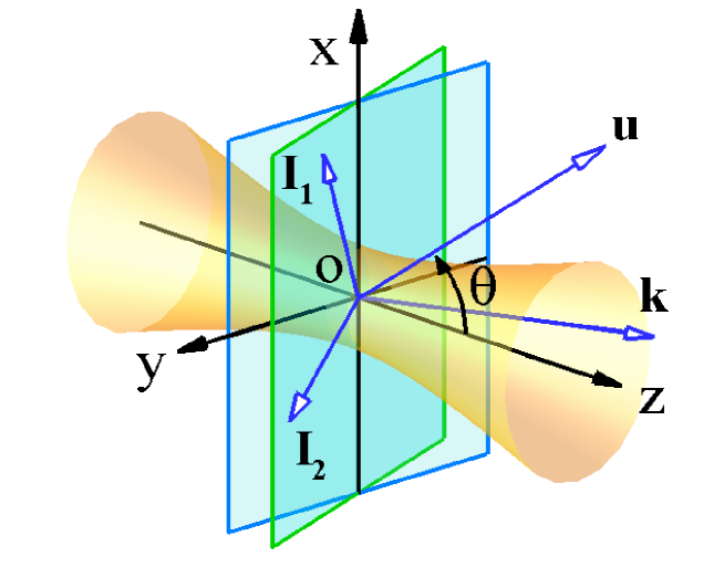
Figure 1: (color online) Schematic illustrating the geometry of the vector field structure. The fixed unit vector $\mathbf{u}$ lies in the plane $zox$ and makes an angle $\theta$ with the propagation axis $z$. The propagation axis $z$ perpendicular to the plane of $xoy$, and the wavevector $\mathbf{k}$ for an arbitrary angular spectrum component is perpendicular to the plane of $I_{1}oI_{2}$

In order to accurately describe the optical Magnus effect, we introduce the scaler Whittaker potentials Pattanayak1980 to represent the vectorial field. Consequently, the angular spectrum can be decomposed along the two vectors and we have

$$\tilde{\mathbf{E}}(k_{x},k_{y})=\tilde{V}_{1}(k_{x},k_{y})\mathbf{I}_{1}+\tilde{V}_{2}(k_{x},k_{y})\mathbf{I}_{2}.$$ (5)

Here $\tilde{V}_{j}=(\alpha~{}~{}~{}\beta)^{T}\tilde{f}(k_{x},k_{y})$ ($j=1,2$) are the scaler Whittaker potentials. The amplitude of the angular spectrum is referred to as

$$\tilde{f}(k_{x},k_{y})=\frac{w_{0}}{\sqrt{2\pi}}\exp\left[-\frac{k_{x}^{2}+k_{y}^{2}}{4}w_{0}^{2}\right],$$ (6)

where $w_{0}$ is beam-waist size. The matrix $(\alpha~{}~{}~{}\beta)^{T}$ denotes the Jones vector which satisfies the normalization condition $\alpha\beta^{\ast}+\alpha^{\ast}\beta=1$. The coefficients $\alpha$ and $\beta$ satisfy the relation $\sigma=i(\alpha\beta^{\ast}-\alpha^{\ast}\beta)$. The polarization operator $\sigma=\pm 1$ corresponds to left and right circularly polarized light, respectively. It is well known that a circularly polarized beam can carry spin angular momentum $\sigma\hbar$ per photon due to its polarization state Beth1936 .

From the viewpoint of Fourier optics Goodman1996 , the Whittaker potentials $V_{j}$ are given by the relation

$$V_{j}(\mathbf{r}) = \frac{1}{k^{2}}\int dk_{x}dk_{y}\tilde{V}_{j}(k_{x},k_{y})$$ (7)

$$\times\exp[i(k_{x}x+k_{y}y+k_{z}z)].$$

It can be verified that both $V_{1}$ and $V_{2}$ satisfy the scalar Helmholtz equation:

$$(\nabla^{2}+k^{2})V_{j}(\mathbf{r})=0.$$ (8)

On substituting Eq. (5) into Eq. (2), the electric field can be expressed in terms of the Whittaker potentials

$$\mathbf{E}(\mathbf{r}) = \nabla\times\nabla\times(\mathbf{u}V_{1})-ik\nabla\times(\mathbf{u}V_{2}).$$ (9)

In fact, after the angular spectrum on the plane $z=0$ is known, Eq. (9) together with Eqs. (4) and (8) provides the expression of the electric field vectors as

$$E_{x}^{[\mathrm{W}]} = \sin\theta\left(k^{2}+\frac{\partial^{2}}{\partial x^{2}}\right)V_{1}+\cos\theta\frac{\partial^{2}V_{1}}{\partial x\partial z}-i\cos\theta k\frac{\partial V_{2}}{\partial y},$$ (10)

$$E_{y}^{[\mathrm{W}]} = \sin\theta\frac{\partial^{2}V_{1}}{\partial x\partial y}+\cos\theta\frac{\partial^{2}V_{1}}{\partial y\partial z}-i\sin\theta k\frac{\partial V_{2}}{\partial z}+i\cos\theta k\frac{\partial V_{2}}{\partial x},$$ (11)

$$E_{z}^{[\mathrm{W}]} = \sin\theta\frac{\partial^{2}V_{1}}{\partial x\partial z}+\cos\theta\left(k^{2}+\frac{\partial^{2}}{\partial z^{2}}\right)V_{1}+i\sin\theta k\frac{\partial V_{2}}{\partial y}.$$ (12)

Here the superscript $[\mathrm{W}]$ represents the vectorial model given by the Whittaker potentials. We find that the electric components can be written as the Whittaker potentials and their first- and second-order derivatives. Up to now, we have established a general propagation model to describe the vector field structure.

It should be noted that the choice of the propagation models in the SHEL has highly debated Onoda2004 ; Bliokh2006 . It is necessary for us to introduce the two polarization models, since optical Magnus effect shares the same physical mechanism with SHEL. Under the paraxial approximation of model $[\mathrm{W}]$, we can get the two different polarization models:

$$\tilde{\mathbf{E}}^{[\mathrm{I}]} \propto \bigg{[}\left(\alpha+\beta\frac{k_{y}}{k}\cot\theta\right)\mathbf{e}_{x}+\left(\beta-\alpha\frac{k_{y}}{k}\cot\theta\right)\mathbf{e}_{y}$$ (13)

$$-\frac{\alpha k_{x}+\beta k_{y}}{k}\mathbf{e}_{z}\bigg{]}\tilde{f}(k_{x},k_{y}),$$

$$\tilde{\mathbf{E}}^{[\mathrm{II}]} \propto \left(\alpha\mathbf{e}_{x}+\beta\mathbf{e}_{y}-\frac{\alpha k_{x}+\beta k_{y}}{k}\mathbf{e}_{z}\right)\tilde{f}(k_{x},k_{y}).$$ (14)

Evidently, model $[\mathrm{II}]$ can be obtained from model $[\mathrm{I}]$ under the condition $\theta=\pi/2$. In the context of wave optics, both model $[\mathrm{I}]$ and model $[\mathrm{II}]$ are exact solutions to the paraxial wave equation. However, the customary paraxial approximation has been shown to be incompatible with the exact Maxwell’s equations Lax1975 . The practical light beams consist of electromagnetic fields and hence are governed by Maxwell’s equations. In recognition of this fact, it is sometimes suggested that the model $[\mathrm{W}]$ representing the Gaussian beam seems to be appropriate. From the experimental viewpoints, even an ideal polarizer will transmit part of a cross-polarized wave Fainman1984 ; Aiello2009b , and thus cannot produce a pure linear polarization state. From the theoretical viewpoints, the linear polarization is a paraxial approximation solution of the Maxwell’s equations. When we go beyond the paraxial approximation and consider the lowest order corrections, the field is elliptical polarization in the cross section Simon1986 ; Simon1987 . Thus, it is desirable to consider the mode $[\mathrm{W}]$ in the optical Magnus effect. As shown in the following, we will compare the results given by the three polarization models.

The changes in the transverse momentum currents can be used to explain the physics behind the rotation phenomenon of the wavepacket, which results in a intensity redistribution over the wavepacket cross section Bekshaev2005 ; Alexeyev2005 . The time-averaged linear momentum density associated with the electromagnetic field can be shown Jackson1999 to be

$$\mathbf{p}^{[\mathrm{M}]}(\mathbf{r})=\frac{1}{2c^{2}}\mathrm{Re}[\mathbf{E}^{[\mathrm{M}]}(\mathbf{r})\times\mathbf{H}^{[\mathrm{M}]\ast}(\mathbf{r})],$$ (15)

Here $\mathrm{M}=\mathrm{W},\mathrm{I},\mathrm{II}$ denotes different polarization models. The magnetic field can be obtained by $\mathbf{H}^{[\mathrm{M}]}=-ik^{-1}\nabla\times\mathbf{E}^{[\mathrm{M}]}$. The momentum currents can be regarded as the combined contributions of spin and orbital parts

$$\mathbf{p}^{[\mathrm{M}]}=\mathbf{p}^{[\mathrm{M}]}_{O}+\mathbf{p}^{[\mathrm{M}]}_{S}.$$ (16)

Here, the orbital term is determined by the macroscopic energy current with respect to an arbitrary reference point and does not depend on the polarization. The spin term, on the other hand, relates to the phase between orthogonal field components and is completely determined by the state of polarization Bekshaev2007 . In a monochromatic optical beam, the spin and orbital currents can be respectively written in the form

$$\mathbf{p}^{[\mathrm{M}]}_{S}=\mathrm{Im}[(\mathbf{E}^{[\mathrm{M}]}\cdot\nabla)\mathbf{E}^{[\mathrm{M}]\ast}],$$ (17)

$$\mathbf{p}^{[\mathrm{M}]}_{O}=\mathrm{Im}[\mathbf{E}^{[\mathrm{M}]\ast}\cdot(\nabla)\mathbf{E}^{[\mathrm{M}]}],$$ (18)

where $\mathbf{E}^{[\mathrm{M}]\ast}\cdot(\nabla)\mathbf{E}^{[\mathrm{M}]}=E_{x}^{[\mathrm{M}]\ast}\nabla E_{x}^{[\mathrm{M}]\ast}+E_{y}^{[\mathrm{M}]\ast}\nabla E_{y}^{[\mathrm{M}]}+E_{z}^{[\mathrm{M}]\ast}\nabla E_{z}^{[\mathrm{M}]}$ is the invariant Berry notation Berry2009 . It has been shown that both spin and orbital currents originate from the beam transverse inhomogeneity and their components are directly related to the azimuthal and radial derivatives of the beam profile parameters. However, the orbital currents are mainly produced by the phase gradient, while the spin currents are orthogonal to the intensity gradient Bekshaev2005 . As shown in the following, the spin and orbital currents will play different roles in the optical Magnus effect.

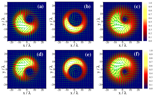
Figure 2: (color online) The momentum currents for the model $[\mathrm{W}]$ under the condition $\theta=\pi/360$. First row: Left circularly polarized wavepacket $\sigma=+1$. Second row: Right circularly polarized wavepacket $\sigma=-1$. The background distribution is depicted as the longitudinal currents and the green arrows is described as the transverse currents. [(a), (d)] Orbital momentum currents $\mathbf{p}_{O}^{[\mathrm{W}]}$. [(b), (e)] Spin momentum currents $\mathbf{p}_{S}^{[\mathrm{W}]}$. [(c), (f)] Total momentum currents $\mathbf{p}_{O}^{[\mathrm{W}]}+\mathbf{p}_{S}^{[\mathrm{W}]}$. The cross section is chosen as $z=z_{R}$ and the intensity is plotted in normalized units.

The monochromatic beam can be formulated as a localized wavepacket whose spectrum is arbitrarily narrow Bliokh2007 . As a mechanical analogy, the circularly polarized wavepacket acts as the rotating ball in our model. To generate an asymmetric intensity distribution, we choose the angle of the fixed unit vector $\mathbf{u}$ as $\theta=\pi/360$. Note that such a vectorial beam should can be realized experimentally without technical difficulties Youngworth2000 ; Ren2006 . In general, the rotation properties of wavepacket are expressed by the transverse momentum currents as shown in Fig. 2. Very surprisingly, the orbital currents are polarization-dependent in this polarization model [Figs. 2(a) and 2(d)]. This is due to the presence of polarization-dependent screw wavefront. For the left circular polarization $\sigma=+1$, the total transverse momentum currents in the exterior part of wavepacket present an anticlockwise circulation, while in the inner part exhibit a clockwise circulation [Fig. 2(c)]. For the right circular polarization $\sigma=-1$, the total transverse momentum currents present an opposite characteristics [Fig. 2(f)]. The inherent physics underlying this intriguing effect is the combined contributions of transverse spin and orbital currents. The wavepacket cannot be regarded as a rigid ball due to the opposite circulations. This is significantly different from the mechanical Magnus effect.

Figure 3: (color online) The momentum currents for the model $[\mathrm{W}]$ under the condition $\theta=\pi/2$. First row: Left circularly polarized wavepacket $\sigma=+1$. Second row: Right circularly polarized wavepacket $\sigma=-1$. The background distribution is depicted as the longitudinal currents and the green arrows is described as the transverse currents. [(a), (d)] Orbital momentum currents $\mathbf{p}_{O}^{[\mathrm{W}]}$. [(b), (e)] Spin momentum currents $\mathbf{p}_{S}^{[\mathrm{W}]}$. [(c), (f)] Total momentum currents $\mathbf{p}_{O}^{[\mathrm{W}]}+\mathbf{p}_{S}^{[\mathrm{W}]}$. The cross section is chosen as $z=z_{R}$ and the intensity is plotted in normalized units.

For the model $[\mathrm{W}]$ under the condition $\theta=\pi/2$, which has also been verified by Hertz vector method Varga1998 , the polarization-dependent rotation of the transverse momentum currents are plotted in Fig. 3. Very interestingly, the orbital currents are polarization-independent in this polarization model [Figs. 3(b) and 3(e)]. However, the transverse spin currents are polarization-dependent and the longitudinal spin currents are absent [Figs. 3(b) and 3(e)]. For the left circular polarization $\sigma=+1$, the total transverse momentum currents present an anticlockwise circulation [Fig. 3(c)]. For the right circular polarization $\sigma=-1$, the total transverse momentum currents present a clockwise circulation [Fig. 3(f)]. The transverse intensity distribution of this model is axially symmetric and the polarization-dependent rotation, if it exists, cannot be observed directly. This is a possible reason why the polarization-dependent split is observed only on the plane which is not perpendicular to the propagation direction of the beam Aiello2009a .

III Optical Magnus Effect

To illustrate the polarization-dependent rotation effect, we now determine the shift of wavepacket centroid, which is given by $\langle\mathbf{r}\rangle^{[\mathrm{M}]}=\langle x\rangle^{[\mathrm{M}]}\mathbf{e}_{x}+\langle y\rangle^{[\mathrm{M}]}\mathbf{e}_{y}$, with

$$\langle\mathbf{r}\rangle^{[\mathrm{M}]}=\frac{\int\int\mathbf{r}p_{z}^{[\mathrm{M}]}(x,y,z)\text{d}x\text{d}y}{\int\int p_{z}^{[\mathrm{M}]}(x,y,z)\text{d}x\text{d}y}.$$ (19)

First let us examine the polarization-dependent rotation in the model $[\mathrm{W}]$. By substituting Eqs. (10), (11) and (15) into Eq. (19), we obtain the shifts as

$$\langle x\rangle^{[\mathrm{W}]}=-\frac{z\sin 2\theta}{2(\cos^{2}\theta+kz_{R}\sin^{2}\theta)},$$ (20)

$$\langle y\rangle^{[\mathrm{W}]}=-\frac{\sigma z_{R}\sin 2\theta}{2(\cos^{2}\theta+kz_{R}\sin^{2}\theta)},$$ (21)

where $z_{R}=kw_{0}^{2}/2$ is the Rayleigh length. We find that the wavepacket centroid shifts a distance away from the propagation axis in $xoy$ plane. The shift $\langle x\rangle^{[\mathrm{W}]}$ is polarization independent, while the shift $\langle y\rangle^{[\mathrm{W}]}$ depends on the polarization state $\sigma$. Note that the shift $\langle x\rangle^{[\mathrm{W}]}$ can be regarded as a small angle inclining from the propagation axis Merano2009 ; Luo2009 . However, the shift $\langle y\rangle^{[\mathrm{W}]}$ does not change on propagation.

The angular positions of the wavepacket centroid indicates the rotation angle $\tan\varphi^{[\mathrm{W}]}=\langle x\rangle^{[\mathrm{W}]}/\langle y\rangle^{[\mathrm{W}]}$, which is significantly different from the previous definition Bekshaev2006 . According to Eq. (19) the rotation angle is given by

$$\varphi^{[\mathrm{W}]}=\arctan\frac{z}{\sigma z_{R}}.$$ (22)

Very surprisingly, the rotation angle is proportional to the Gouy phase for circular polarization $\sigma=\pm 1$. In all cross sections denoted by the distance from the $z=0$ plane, the transverse patterns are quite similar. However the overall scale changes and the pattern rotates as a whole. The former is caused by diffraction, and the latter is seen due to the existence of transverse momentum currents.

Since the rotating wavepacket passes the distance between different cross-sections in time $t=z/c$, the instant angular velocity can be given by $\Omega^{[\mathrm{W}]}(z)=d\varphi^{[\mathrm{W}]}/dt=cd\varphi^{[\mathrm{W}]}/dz$, so that

$$\Omega^{[\mathrm{W}]}(z)=c\frac{\sigma z_{R}}{\sigma^{2}z_{R}^{2}+z^{2}}.$$ (23)

The rotation velocity of the wavepacket centroid decreases as the propagation distance increases. When the condition $\sigma=0$ is satisfied and the rotation characteristics of wavepacket centroid vanish, i.e., $\Omega^{[\mathrm{W}]}(z)=0$. This is why the linear polarized wavepacket cannot present the optical Magnus effect. However the linear polarization can be represented as a superposition of two circularly polarized components Bliokh2006 . As the result, the polarization-dependent split of the wavepacket intensity distribution arises. Thus, the same mechanism also leads to other effects such as the SHEL.

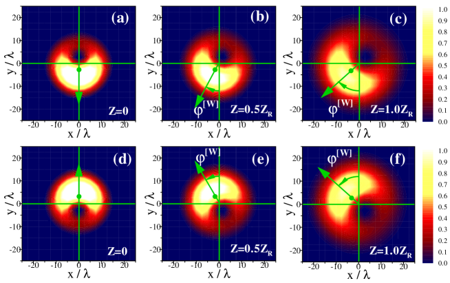
Figure 4: (color online) The polarization-dependent rotations of wavepacket centroid (green point) for the model $[\mathrm{W}]$. First row: The wavepacket centroid undergoes a clockwise rotation for left circular polarization $\sigma=+1$. Second row: The wavepacket centroid presents an anticlockwise rotation for right circular polarization $\sigma=-1$. Images are labeled by corresponding values of propagation length $z$ and rotation angle $\varphi^{[\mathrm{W}]}$. The intensity distributions are plotted in the plane [(a), (d)] $z=0$, [(b), (e)] $z=0.5z_{R}$, and [(c), (f)] $z=z_{R}$. Other parameters are the same as those in Fig. 2.

Figure 4 shows the polarization-dependent rotations of wavepacket centroid. At the plane $z=const.$, the intensity of the wavepacket can be regarded as $I^{[\mathrm{W}]}(\mathbf{r})=c^{2}p^{[\mathrm{W}]}_{z}(\mathbf{r})$. The wavepacket centroid (green spots) whose angular positions indicate the rotation angle $\varphi$. For the left circular polarization $\sigma=+1$, the wavepacket centroid exhibits a clockwise rotation [Figs. 4(a)-4(c)]. For the right circular polarization $\sigma=-1$, however, the wavepacket centroid presents an anticlockwise rotation [Figs. 4(d)-4(f)]. During the wavepacket propagation from $z=0$ to $z=+z_{R}$, the rotation angle amounts to $\varphi^{[\mathrm{W}]}=\sigma\pi/4$. The physics underlying this intriguing effect is the combined contributions of transverse spin and orbital currents. The novel polarization-dependent rotations differs from the conventional optical Magnus effect, in that light-matter interaction is not required.

We are currently investigating the polarization mode $[\mathrm{I}]$. On substituting Eqs. (2) and (13) into Eq. (19) we have

$$\langle x\rangle^{[\mathrm{I}]}=0~{}~{}~{}~{}~{}\langle y\rangle^{[\mathrm{I}]}=-\frac{\sigma\cot\theta}{k}.$$ (24)

There exists an inherent transverse shift on propagation. This result coincides with that obtained by Li Li2009a with different methods. According to Eq. (24) the rotation angle is given by

$$\varphi^{[\mathrm{I}]}=\sigma\arctan\frac{\pi}{2}.$$ (25)

In this case, the rotation characteristics of wavepacket centroid vanish, i.e., $\Omega^{[\mathrm{I}]}(z)=0$.

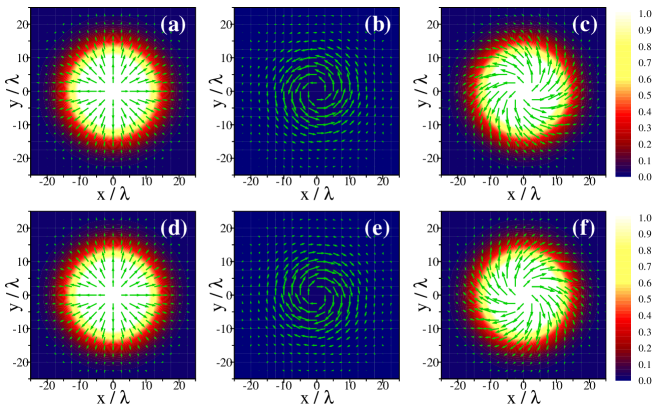
Figure 5: (color online) The polarization-dependent rotations of transverse momentum currents for the model $[\mathrm{II}]$. First row: Left circularly polarized wavepacket $\sigma=+1$. Second row: Right circularly polarized wavepacket $\sigma=-1$. The background distribution is depicted as the longitudinal currents and the green arrows is described as the transverse currents. [(a), (d)] Orbital momentum currents $\mathbf{p}_{O}^{[\mathrm{II}]}$. [(b), (e)] Spin momentum currents $\mathbf{p}_{S}^{[\mathrm{II}]}$. [(c), (f)] Total momentum currents $\mathbf{p}_{O}^{[\mathrm{II}]}+\mathbf{p}_{S}^{[\mathrm{II}]}$. The cross section is chosen as $z=z_{R}$ and the intensity is plotted in normalized units.

We are now in a position to consider the polarization model $[\mathrm{II}]$. On substituting Eqs. (2) and (14) into Eq. (19) we can determine

$$\langle x\rangle^{[\mathrm{II}]}=0,~{}~{}~{}~{}~{}\langle y\rangle^{[\mathrm{II}]}=0.$$ (26)

A further important point should be noted is that Eq. (26) can be obtained from Eq. (24) under the condition $\theta=\pi/2$. In this model, the polarization-dependent rotation of the centroid cannot be observed directly. Thus, we attempt to explore an alternative way to describe the polarization-dependent rotation effect. When the momentum currents are included, the change rate of azimuthal angle with $z$ axis is written as Padgett1995

$$\frac{\partial\varphi^{[\mathrm{II}]}}{\partial z}=\frac{p_{\varphi}^{[\mathrm{II}]}}{rp_{z}^{[\mathrm{II}]}}.$$ (27)

Here, $p_{\varphi}$ describes the momentum current that circulates around the propagation axis, and $p_{z}$ describes the momentum current that propagates along the $+z$ axis. The result of Eq. (15) can be expressed in term of azimuthal component, defined by

$$p_{\varphi}^{[\mathrm{II}]}=-p_{x}^{[\mathrm{II}]}\sin\varphi+p_{y}^{[\mathrm{II}]}\cos\varphi,$$ (28)

By substituting Eqs. (15) and (28) into Eq. (27) and carrying out the integration, we obtain

$$\varphi^{[\mathrm{II}]}=\sigma\arctan\frac{z}{z_{R}}.$$ (29)

This result is slightly different from the rotation of the centroid in model $[\mathrm{W}]$. The instant angular velocity can be given by $\Omega^{[\mathrm{II}]}(z)=cd\varphi^{[\mathrm{II}]}/dz$, so that

$$\Omega^{[\mathrm{II}]}(z)=c\frac{\sigma z_{R}}{z_{R}^{2}+z^{2}}.$$ (30)

The rotation velocity of the momentum current decreases as the propagation distance increases. When the condition $\sigma=0$ is satisfied, the rotation characteristics vanish.

To obtain a clear physical picture, the polarization-dependent rotations of the momentum currents are plotted in Fig. 5. We find that the orbital currents are polarization-independent in this polarization model [Figs. 5(a) and 5(d)]. However, the spin currents are polarization-dependent [Figs. 5(b) and 5(e)]. For the left circular polarization $\sigma=+1$, the total transverse momentum currents present an anticlockwise circulation [Fig. 5(c)]. For the right circular polarization $\sigma=-1$, the total transverse momentum currents present a clockwise circulation [Fig. 5(f)]. The polarization-dependent rotations of momentum currents may provide an alternative way to illustrate the optical Magnus effect, although whether the momentum currents in the free space propagating along a curvilinear trajectory is still debated Allen2000 ; Volyar1999 . Comparing Fig. 3 with Fig. 5 shows that there are no notable difference between the model $[\mathrm{W}]$ (under the condition $\theta=\pi/2$) and the model $[\mathrm{II}]$. In fact, the latter can be regarded as the paraxial approximation of the former.

IV Spin and orbital angular momenta

In the frame of classical electrodynamics, it is the circularly polarized wavepacket but not the spin photon acting as the rotating ball. Now a question arises: What roles the spin and orbital angular momenta play in the optical Magnus effect? We now in the position to analysis the angular momentum density for each of individual wavepacket, which can be written as Jackson1999

$$\mathbf{j}^{[\mathrm{M}]}(\mathbf{r})=\mathbf{r}\times\mathbf{p}^{[\mathrm{M}]}(\mathbf{r}).$$ (31)

Within the paraxial approximation, the angular momentum can be divided into the spin and orbital angular parts $\mathbf{j}^{[\mathrm{M}]}=\mathbf{j}^{[\mathrm{M}]}_{O}+\mathbf{j}^{[\mathrm{M}]}_{S}$ Allen1992 , it follows that

$$\mathbf{j}^{[\mathrm{M}]}_{O}=\mathbf{r}\times\mathbf{p}^{[\mathrm{M}]}_{O},$$ (32)

$$\mathbf{j}^{[\mathrm{M}]}_{S}=\mathbf{r}\times\mathbf{p}^{[\mathrm{M}]}_{S}.$$ (33)

This separation should hold beyond the paraxial approximation Barnett2002 .

We first consider the longitudinal angular momentum density $j_{z}$ which can be regarded as the combined contributions of spin and orbital parts:

$$j^{[\mathrm{M}]}_{\mathrm{Oz}}=xp^{[\mathrm{M}]}_{Oy}-yp^{[\mathrm{M}]}_{Ox},$$ (34)

$$j^{[\mathrm{M}]}_{Sz}=xp^{[\mathrm{M}]}_{Sy}-yp^{[\mathrm{M}]}_{Sx}.$$ (35)

The longitudinal angular momentum will provide a simple way to understand why the circularly polarized wavepacket exhibits the optical Magnus effect.

Figure 6 presents the distribution of longitudinal angular momentum density for the model $[\mathrm{W}]$. Very surprisingly, this polarization model of wavepacket possesses polarization-dependent orbital angular momentum density [Figs. 6(a) and 6(d)]. However, the spin momentum density exhibits a significantly different distribution [Figs. 6(b) and 6(e)]. For the left circular polarization $\sigma=+1$, the total angular momentum density in the exterior part of wavepacket is positive $j_{z}>0$, while in the inner part is negative $j_{z}<0$ [Fig. 6(c)]. This means that the outer part of the packet presents an anticlockwise rotation, the inner part undergoes a clockwise one. For the right circular polarization $\sigma=-1$, the total angular momentum density of wavepacket presents an oppositive distribution [Fig. 6(f)]. Thus, the rotating wavepacket cannot be regarded as a rigid ball as in the mechanical Magnus effect. This is the reason why we choose the centroid as the reference point to describe the polarization-dependent trajectories.

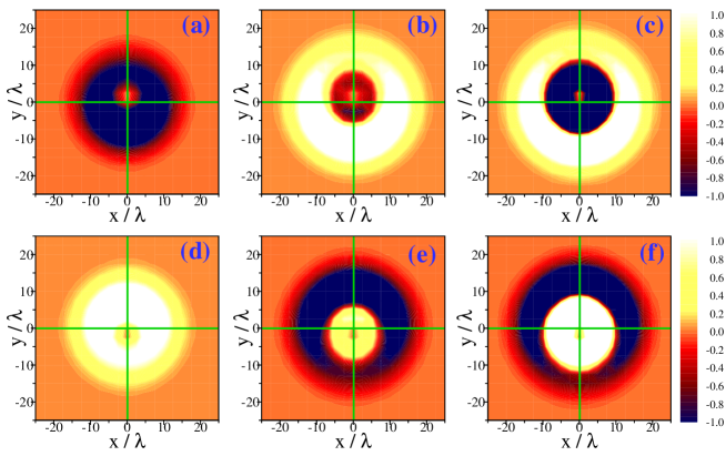
Figure 6: (color online) The distribution of the longitudinal angular momentum density for the model $[\mathrm{W}]$. First row: Left circular polarization $\sigma=+1$. Second row: Right circular polarization $\sigma=-1$. [(a), (d)] Orbital angular momentum density $j_{Oz}^{[\mathrm{W}]}$. [(b), (e)] Spin angular momentum density $j_{Sz}^{[\mathrm{W}]}$. [(c), (f)] Total angular momentum density $j_{Oz}^{[\mathrm{W}]}+j_{Sz}^{[\mathrm{W}]}$. The cross section is chosen as $z=0$ and the intensity is plotted in normalized units. Other parameters are the same as those in Fig. 2.

For the comparison, we plot the longitudinal momentum density of the model $[\mathrm{II}]$ in Fig. 7. By comparing with the model $[\mathrm{W}]$, we find that the orbital angular momentum density vanishes in the present polarization model [Figs. 7(a) and 7(d)]. Thus, only the spin momentum density exhibits a polarization-dependent distribution [Figs. 7(b) and 7(e)]. For the left circular polarization $\sigma=+1$, the total angular momentum density first increases then decreases with the increase of $r$ as shown in Fig. 7(c). For the right circular polarization $\sigma=-1$, the total angular momentum density presents an oppositive distribution as shown in Fig. 7(f). The transverse intensity distribution is axially symmetric and the polarization-dependent rotation, if it exists, cannot be observed directly.

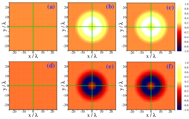
Figure 7: (color online) The distribution of the longitudinal angular momentum density for the model $[\mathrm{II}]$. First row: Left circular polarization $\sigma=+1$. Second row: Right circular polarization $\sigma=-1$. [(a) and (d)] Orbital angular momentum density $j_{Oz}^{[\mathrm{II}]}$. [(b) and (e)] Spin angular momentum density $j_{Sz}^{[\mathrm{II}]}$. [(c) and (f)] Total angular momentum density $j_{Oz}^{[\mathrm{II}]}+j_{Sz}^{[\mathrm{II}]}$. The cross section is chosen as $z=0$ and the intensity is plotted in normalized units. Other parameters are the same as those in Fig. 5.

Now we want to enquire what roles the angular momentum play in the optical Magnus effect. To answer this question needs to discuss the transverse angular momentum. The time-averaged linear momentum and angular momentum, which can be obtained by integrating over the whole $x-y$ plane Jackson1999

$$\mathbf{P}^{[\mathrm{M}]}=\int\int\mathbf{p}^{[\mathrm{M}]}(\mathbf{r})\text{d}x\text{d}y,$$ (36)

$$\mathbf{J}^{[\mathrm{M}]}=\int\int\mathbf{j}^{[\mathrm{M}]}(\mathbf{r})\text{d}x\text{d}y.$$ (37)

The transverse angular momentum components are given by

$$J^{[\mathrm{M}]}_{x}=\langle y\rangle P^{[\mathrm{M}]}_{z}-zP^{[\mathrm{M}]}_{y},$$ (38)

$$J^{[\mathrm{M}]}_{y}=zP^{[\mathrm{M}]}_{x}-\langle x\rangle P^{[\mathrm{M}]}_{z}.$$ (39)

In the $z=0$ plane, we have $J_{x}^{[\mathrm{M}]}/P_{z}^{[\mathrm{M}]}=\langle y\rangle^{[\mathrm{M}]}$ and $J_{y}^{[\mathrm{M}]}/P_{z}^{[\mathrm{M}]}=-\langle x\rangle^{[\mathrm{M}]}$. Thus, the transverse angular momentum can be obtained by measuring the position of wavepacket centroid Aiello2009a . In order to reveal the rotation characteristics, it is necessary for us to know the transverse angular momentum in any cross section. We first consider the model $[\mathrm{W}]$, the transverse angular momenta are given by

$$J^{[\mathrm{W}]}_{x}=-\frac{\pi\sigma\sin 2\theta}{2k^{2}z_{R}},~{}~{}~{}~{}~{}J^{[\mathrm{W}]}_{y}=\frac{\pi z\sin 2\theta}{2k^{2}z_{R}^{2}}.$$ (40)

In this case, the polarization-dependent rotation of the centroid is unavoidable since the wavepacket possesses transverse angular momentum. For the model $[\mathrm{I}]$, we obtain

$$J^{[\mathrm{I}]}_{x}=-\frac{\pi\sigma\cot\theta}{k^{2}z_{R}},~{}~{}~{}~{}~{}~{}J^{[\mathrm{I}]}_{y}=0.$$ (41)

This is the reason why the model $[\mathrm{I}]$ only exhibits a transverse shift. For the model $[\mathrm{II}]$, however

$$J^{[\mathrm{II}]}_{x}=0,~{}~{}~{}~{}~{}~{}J^{[\mathrm{II}]}_{y}=0.$$ (42)

Thus, the wavepacket centroid no longer presents the polarization-dependent rotation. The physics underlying this phenomenon is the absence of the transverse angular momentum. It should be noted that the SHEL can be noticeably enhanced when the wavepacket carries orbital angular momentum Bliokh2009a ; Bliokh2009b ; Fadeyeva2009 . Further work is needed to uncover the optical Magnus effect of such a wavepacket in the free space.

It should be mentioned that the recent advent of negative index metamaterials, also known as left-handed materials (LHMs) Veselago1968 ; Shelby2001 , can induce a reversed polarization-dependent rotation of the trajectory of the wavepacket centroid. Because of the negative index, we can expect a negative Rayleigh length in LHMs Luo2008a ; Luo2008b . It will be interesting for us to describe in detail how the wavepacket trajectory evolves in the LHMs. Recently, the technique of transformation optics has emerged as a means of designing metamaterials that can bring about unprecedented control of electromagnetic fields Pendry2006 . It is possible that the trajectories of circularly polarized wavepacket can be controlled by introducing a prescribed spatial variation in the constitutive parameters.

V Conclusions

In conclusion, we have established a general vector field model to describe the role of transverse momentum currents in optical Magnus effect in the free space. We have demonstrated the existence of a novel optical polarization-dependent Magnus effect which differs from conventional optical Magnus effect in that light-matter interaction is not required. In the optical Magnus effect, the circularly polarized wavepacket acts as the rotating ball, but is not identical to a rigid body. This is because different parts of the wavepacket present diverse rotation characteristics. For a certain circularly polarized wavepacket, whether the rotation is clockwise or anticlockwise depends on the polarization state. Such a polarization-dependent rotation is unavoidable when the wavepacket possesses transverse momentum currents. We predict that this novel effect may be observed experimentally even in the propagation direction. Our findings provide further evidence for the optical Magnus effect in the free space. Because of the close similarity in atom physics, condensed matter, and optical physics, we believe that the Magnus effect is not limited to electromagnetic fields, but extends to other research areas, such as atom, ion, and electron beams.

- (1) A. V. Dooghin, N. D. Kundikova, V. S. Liberman, and B. Y. Zeldovich, Phys. Rev. A 45, 8204 (1992).
- (2) V. S. Liberman and B. Y. Zeldovich, Phys. Rev. A 46, 5199 (1992).
- (3) K. Y. Bliokh, A. Niv, V. Kleiner, and E. Hasman, Nature Photon. 2, 748 (2008).
- (4) O. S. Borodavka, A. V. Volyar, V. G. Shvedov, and S. A. Reshetnicoff, Proc. SPIE, 3904, 55 (1999).
- (5) D. N. Pattanayak and G. P. Agrawal, Phys. Rev. A 22, 1159 (1980).
- (6) M. Onoda, S. Murakami, and N. Nagaosa, Phys. Rev. Lett. 93, 083901 (2004).
- (7) K. Y. Bliokh and Y. P. Bliokh, Phys. Rev. Lett. 96, 073903 (2006).
- (8) O. Hosten and P. Kwiat, Science 319, 787 (2008).
- (9) D. Haefner, S. Sukhov, and A. Dogariu, Phys. Rev. Lett. 102, 123903 (2009).
- (10) A. Aiello, N. Lindlein, C. Marquardt, and G. Leuchs, Phys. Rev. Lett. 103, 100401 (2009).
- (11) C. F. Li, Phys. Rev. A 79, 053819 (2009).
- (12) C. F. Li, Phys. Rev. A 80, 063814 (2009).
- (13) L. W. Davis, Phys. Rev. A 19, 1177 (1979).
- (14) L. W. Davis and G. Patsakos, Opt. Lett. 6, 22 (1981).
- (15) R. A. Beth, Phys. Rev. 50, 115 (1936).
- (16) J. W. Goodman, Introduction to Fourier Optics (McGraw-Hill, New York, 1996).
- (17) M. Lax, W. H. Louisell, and W. McKnight, Phys. Rev. A 11, 1365 (1975).
- (18) Y. Fainman and J. Shamir, Appl. Opt. 23, 3188 (1984).
- (19) A. Aiello, C. Marquardt, and G. Leuchs, Opt. Lett. 34, 3160 (2009).
- (20) R. Simon, E. C. G. Sudarshan, and N. Mukunda, J. Opt. Soc. Am. A 3, 536 (1986).
- (21) R. Simon, E. C. G. Sudarshan, and N. Mukunda, Appl. Opt. 26, 1589 (1987).
- (22) A. Yu. Bekshaev, M. S. Soskin, and M. V. Vasnetsov, Opt. Commun. 249, 367 (2005).
- (23) C. N. Alexeyev and M. A. Yavorsky, J. Opt. A: Pure Appl. Opt. 7, 416 (2005).
- (24) J. D. Jackson, Classical Electrodynamics (Wiley, New York, 1999).
- (25) A. Y. Bekshaev and M. S. Soskin, Opt. Commun. 271, 332 (2007).
- (26) M. V. Berry, J. Opt. A: Pure Appl. Opt. 11, 094001 (2009).
- (27) K. Y. Bliokh and Y. P. Bliokh, Phys. Rev. E 75, 066609 (2007).
- (28) K. S. Youngworth and T. G. Brown, Opt. Express 7, 77 (2000).
- (29) H. Ren, Y. H. Lin, and S. T. Wu, Appl. Phys. Lett. 89, 051114 (2006).
- (30) P. Varga and P. Török, Opt. Commun. 152, 108 (1998).
- (31) M. Merano, A. Aiello, M. P. van Exter, and J. P. Woerdman, Nature Photon. 3, 337 (2009).
- (32) H. Luo, S. Wen, W. Shu, Z. Tang, Y. Zou, and D. Fan, Phys. Rev. A 80, 043810 (2009).
- (33) A. Bekshaev and M. Soskin, Opt. Lett. 31, 2199 (2006).
- (34) M. J. Padgett and L. Allen, Opt. Commun. 121, 36 (1995).
- (35) L. Allen and M. J. Padgett, Opt. Commun. 184, 67 (2000).
- (36) A. V. Volyar, V. G. Shvedov, and T. A. Fadeeva, Tech. Phys. Lett. 25, 203 (1999).
- (37) L. Allen, M. W. Beijersbergen, R. J. C. Spreeuw, and J. P. Woerdman, Phys. Rev. A 45, 8185 (1992).
- (38) S. M. Barnett, J. Opt. B 4, S7 (2002).
- (39) K. Y. Bliokh, and A. S. Desyatnikov, Phys. Rev. A 79, 011807(R) (2009).
- (40) K. Y. Bliokh, I. V. Shadrivov, and Y. S. Kivshar, Opt. Lett. 34, 389 (2009).
- (41) T. A. Fadeyeva, A. F. Rubass, and A. V. Volyar, Phys. Rev. A 79, 053815 (2009)
- (42) V. G. Veselago, Sov. Phys. Usp. 10, 509 (1968).
- (43) R. A. Shelby, D. R. Smith, and S. Schultz, Science 292, 77 (2001).
- (44) H. Luo, Z. Ren, W. Shu, and S. Wen, Phys. Rev. A 77, 023812 (2008).
- (45) H. Luo, S. Wen, W. Shu, Z. Tang, Y. Zou, and D. Fan, Phys. Rev. A 78, 033805 (2008).
- (46) J. Pendry, D. Schurig, and D. Smith, Science 312, 1780 (2006).