Parity and Cobordisms of Free Knots

Abstract

In the present paper, we construct a simple invariant which provides a sliceness obstruction for free knots. This obstruction provides a new point of view to the problem of studying cobordisms of curves immersed in $2$-surfaces, a problem previously studied by Carter, Turaev, Orr, and others.

The obstruction to sliceness is constructed by using the notion of parity recently introduced by the author into the study of virtual knots and their modifications. This invariant turns out to be an obstruction for cobordisms of higher genera with some additional constraints.

AMS Subject Classification: 57M25.

1 Introduction

Curves immersed in 2-surfaces admit a natural notion of cobordisms: one says that two curves $\gamma$ and $\gamma^{\prime}$ immersed in oriented closed $2$-surfaces (not necessarily connected, but for the sake of simplicity we shall use the notation for connected surfaces) $S_{g}$ and $S_{g^{\prime}}$, are cobordant if there is an oriented $3$- manifold $M$ whose boundary consists of two surfaces $S^{+}_{g}=S_{g}$ and $S^{-}_{g^{\prime}}=S_{g^{\prime}}$ and a properly smoothly mapped cylinder $C\subset M$, such that $\partial C=C\cap\partial M$ and $C\cap S^{+}_{g}=\gamma,C\cap S^{-}_{g^{\prime}}=\gamma^{\prime}$, see Fig. 1.

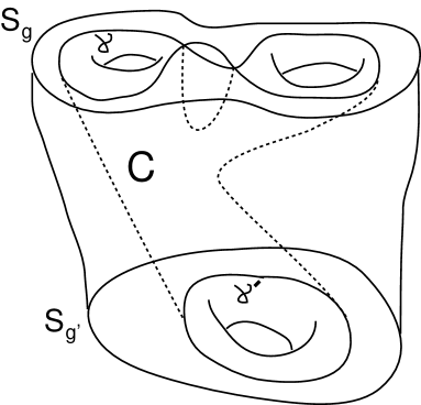
Figure 1: A cobordism between immersed curves

In particular, one says that a curve $\gamma\in S_{g}$ is null-cobordant (or slice) whenever there is an oriented $3$-manifold $M,\partial M=S_{g}$ and a disc $D$ properly immersed in $M$ by a map $f$ such that $f(\partial D)=f(D)\cap\partial M=\gamma$.

Analogously, one says that the slice genus of $\gamma\subset S_{g}$ does not exceed $h$ if in the above definition one uses a surface $D_{h}$ of genus $h$ with one boundary component instead of the disc $D$.

The cobordism is obviously an equivalence relation; cobordism classes of curves form a group (with connected sum playing the role of multiplication) where the equivalence class of null-cobordant elements play the role of unity.

The first obstructions for curves to be null-cobordant were found by Carter, [2]; after that, the theory was also studied by Turaev [12], Orr, and others.

• 1. In the sequel, we deal only with generic immersions of curves in $2$-surfaces, unless specified otherwise.

It can be easily proved that if two curves $\gamma,\gamma^{\prime}\subset S_{g}$ are homotopic then they are cobordant, so one can talk about cobordism classes of homotopy classes of curves.

Thus, it is natural to talk about cobordism classes of flat virtual knots (virtual strings) [11], which are equivalence classes of circle immersions in $2$-surfaces considered up to homotopy and stabilization/destabilization. The stabilization operation (addition of a handle to $S_{g}$ away from the curve) obviously does not change the cobordism class of the curve.

The paper [6] (full versions see in [5]) pioneered the overall study of free knots, which are formal equivalence classes of framed $4$-graphs with modulo the three Reidemester moves. The free knots are a thorough simplifiaction of virtual knots, moreover, the are a simplification of flat virtual knots as well, since they can be obtained from the latter by “forgetting the surface structure”.

In [6], the first examples of non-trivial free knots were constructed, and some properties were established. Some days afterwards, non-trivial free knots were constructed by Gibson [3]. The key notion used in many constructions from [5, 6, 7] is the notion of parity, which allows one to solve several problems, construct new invariants of (virtual) knots and their relatives, strengthen some known invariants, and construct maps from knots to knots.

Once it is proved that free knots are generally non-trivial, the question of non-sliceness of free knots arose; rigorous definitions of the slice genus see ahead in Definition 4.

Informally speaking, before constructing an invariant of some topological objects, one should first look at some “building bricks” or “nodes” of these objects (like crossings of a knot diagram or intersection points of a curve generically immersed in a $2$-surface or intersection lines of a $2$-surfaces immersed in a $3$-manifold), and try to figure out whether one can distinguish between different types of them by looking at the global topology/combinatorics of our object. Then, one may try to modify existing combinatorial invariants (or to construct new ones) by adding this extra information into a given setup.

In the context of free knots all vertices of the four-graph can be naturally split into the set of “even ones” and “odd ones”.

It is clear that every invariant of free knots generates an invariant of flat virtual knots (one just has to take its composition with a natural “forgetting projection”). So, for free knots one can naturally define the notion of cobordism in a way such that that if two flat virtual knots are cobordant then so are the underlying free knots.

On the other hand, cobordism invariants constructed by Carter, Orr, Turaev, and others can not be straightforwardly defined for the case of free knots, since they use some homological data of the surface, which free knots do not possess. In some sense, parity can substitute homological/homotopy information, when there is no “genuine” homology.

The concept of parity has some other applications in the cobordism theory for free knots/immersed curves. In particular, if a free knot $\gamma$ is slice, then so is the free knot $\gamma^{\prime}$ obtained from $\gamma$ by “killing odd crossings”, see Theorem 5 ahead.

The aim of the present paper is to construct one simple (in fact, integer-valued) invariant of free knots which gives an obstruction for a free knot to be slice (null-cobordant).

The paper is organized as follows. First we define free knots, parity, Gaussian parity and construct our invariant. We prove its invariance under Reidemeister moves. Then, to show that the invariant is well-behaved under cobordisms, we have to extend the notion of parity from one knot to the spanning disc of the cobordism. This is done by marking double lines of the spanning disc as “even” and “odd”. After that we give the basic definitions of Morse theory for cobordisms, and outline the proof of the main theorem. Taking a Morse function on a spanning disc, one extends the invariant to all the regular sections of this function, and the non-triviality of the initial invariant coupled with simple Morse theoretic arguments leads to a contradiction. The key point in the proof is the way to extend the notion of parity from vertices of $4$-graphs to double lines of $2$-surfaces.

We conclude the paper by a list of further possible developments of this theory of parity and cobordisms. In particular, the approach described in the present paper is good for detecting non-sliceness but is not (in its original form) applicable for getting estimates of the slice genus because of some caveats relating parity and Morse theory.

On the other hand, the concept of parity evidently has multidimensional analogues and may be applied for $2$-knots in $4$-space and similar objects. Our last section initiates a discussion of problems of such sort.

In [4] some other relation called cobordisms of free knots was discussed: instead of topological definition obtained by considering spanning discs, we dealt with a formal combinatorial definition following Turaev which relies on a set of moves. An invariant of combinatorial cobordism was constructed.

The interrelation between these two equivalence relations, topological cobordisms and combinatorial cobordisms, will be considered in a future publication.

1.1 Acknowledgement

My study of free knots and their cobordisms was initiated after I got deeply impressed by a talk “Surface Knots and Iterated Intersection Pairings” by Kent E.Orr given at a conference in Heidelberg in 2008 about a deep connection between cobordisms of curves in $2$-surfaces and cobordisms of knots. The obstruction (due to Carter and later, its expansion due to Turaev and Orr) was based on homological information about the surface in question. This lead me to an idea of finding a good “substitute” for homology when instead of a curve in a $2$-surface one has an abstract curve with self-intersection.

Various discussions with Kent Orr led me to a deeper understanding of many results in this area, and I am deeply indebted to him.

I express my gratitude to L.H.Kauffman, D.P.Ilyutko and M.Chrisman for fruitful consultations.

1.2 Free Knots

By a graph we always mean a finite (multi)graph; loops and multiple edges are allowed. From now on, by a $4$-graph we mean the following generalization of a four-valent graph: a $1$-dimensional complex $\Gamma$, with each connected component being homeomorphic either to the circle (with no matter how many $0$-cells) or to a four-valent graph; by a vertex we shall mean only vertices of those components which are homeomorphic to four-valent graphs, and by edges we mean either edges of four-valent-graph-components or circular components; the latter will be called cyclic edges.

We say that a $4$-graph is framed if for every vertex of it, the four emanating half-edges are split into two pairs. We call the half-edges from the same pair opposite. We shall also apply the term opposite to edges containing opposite half-edges.

By isomorphism of framed $4$-graphs we assume a framing-perserving homeomorphism. All framed $4$-graphs are considered up to isomorphism.

Denote by $G_{0}$ the framed $4$-graph homeomorphic to the circle.

By a unicursal component of a framed $4$-graph we mean either its connected component homeomorphic to the circle or an equivalence class of its edges, where the equivalence is generated by the relation of being opposite.

By a chord diagram we mean a cubic graph consisting of one selected cycle passing through all vertices of the graph and a set of chords. We call this cycle the core of the chord diagram. A chord diagram is oriented whenever its circle is oriented. Edges belonging to the core cycle are called arcs of the chord diagram.

Let $D$ be a chord diagram. Then the corresponding $4$-graph $G(D)$ with a unique unicrusal component is constructed as follows. If the set of chords of $D$ is empty then the corresponding graph will be $G_{0}$. Otherwise, the edges of the graph are in one-to-one correspondence with arcs of the chord diagram, and vertices are in one-to-one correspondence with chords of the chord diagram. The arcs incident to the same chord end, correspond to the (half)-edges which are formally opposite at the vertex corresponding to the chord. We say that two chords $a$ and $b$ of a chord diagram $D$ are linked, if the ends of the chord $b$ belong to different connected components of the complement to the ends of $a$ in the core circle $C$. In this case we write $\langle a,b\rangle=1$. Otherwise we say that chords are unlinked and write $\langle a,b\rangle=0$.

The inverse procedure (of constructing a chord diagram from a framed $4$-graph) with one unicursal component is evident. In this situation every connected framed $4$-graph can be considered as a topological space obtained from the circle by identifying some pairs of points. Thinking of the circle as the core circle of a chord diagram, where the pairs of identified chords will correspond to chords, one obtains a chord diagram.

For a framed $4$-graph $G$ with one unicursal component we define the ${\mathbb{Z}}_{2}$-pairing of vertices vertices $v_{1},v_{2}$ as follows: $\langle v_{1},v_{2}\rangle=\langle a(v_{1}),a(v_{2})\rangle$, where $a(v_{1}),a(v_{2})$ are chords corresponding to the vertices $v_{1},v_{2}$.

Our first aim is to study equivalence classes of framed four graphs modulo some moves corresponding to Reidemeister moves for knots, cf. [5].

Each of this moves is a transformation of one fragment of a framed $4$-graph.

Graphical notation. In figures depicting moves on diagrams, we shall draw only the changing part; the stable part will be omitted. In the case of one unicursal component a move can be represented by Gauss diagram; the move changes the diagram on some set of arcs; we shall not draw those chords away from the Reidemeister move being performed; the arcs having no ends of chords taking part in the move, will be depicted by dotted lines.

When drawing framed graphs on the plane, we always assume that the opposite half-edges structure is induced from the plane.

The first Reidemeister move is an addition/removal of a loop, see Fig.2.

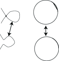
Figure 2: The first Reidemeister move and its chord diagram version

The second Reidemeister move is an addition/removal of a bigon formed by a pair of edges which are adjacent (not opposite) in each of the two vertices, see Fig. 3. It has two variants; nevertheless, it can be easily seen, that any of these two variants is expressed as a combination of the other one and the second Reidemeister moves.

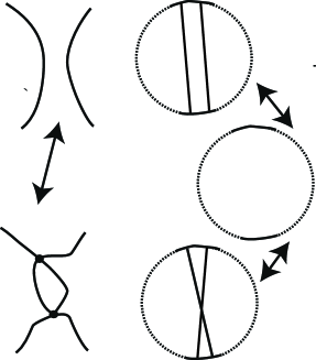
Figure 3: The second Reidemeister move and its chord diagram version

The third Reidemeister move is shown in Fig. 4.

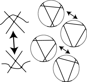
Figure 4: The third Reidemeister move and its chord diagram version

• 2. A free link is an equivalence class of framed 4-graphs modulo Reidemeister moves.

  It is evident that the number of components of a framed 4-graph does not change after applying a Reidemeister move, so, it makes sense to talk about the number of components of a free link.

  By a free knot we mean a free link with one unicursal component.

  Free knots can be treated as equivalence classes of Gauss diagrams by moves corresponding to Reidemeister moves.

The free unknot (resp., free $n$-component unlink) is the free knot (link) represented by $G_{0}$ (resp., by $n$ disjoint copies of $G_{0}$).

Analogously one defines long free knots; here one should break the only component and pull its ends to infinity; all graphs; all moves are considered in finite domains. Equivalently, we may consider a $4$-valent graph with one unicursal component with a marked edge up to the Reidemeister moves performed away from the marked point.

1.3 The Parity Axiomatics. The Gaussian Parity

We define the key properties of parity for free knots by using a set of axioms, following [5].

• 3. A parity is a map assigning to each pair $(\Gamma,V)$, where $\Gamma$ is a framed $4$-graph and $V$ is a vertex of $\Gamma$, a number $p(V)$ (also denoted by $p_{\Gamma}(V)$) which is equal to $0\in{\mathbb{Z}}_{2}$ (in this case the vertex $V$ is called even) or $1\in{\mathbb{Z}}_{2}$ (when the vertex is called odd) in such a way that this rule satisfies the following axioms.

  1. If a framed $4$-graph $K_{2}$ is obtained from a framed $4$-graph $K_{1}$ by a first (decreasing) Reidemeister move then the crossing of $K_{1}$ taking part in the Reidemeister move is even;

  2. If $K_{2}$ is obtained from $K_{1}$ by a second Reidemeister move then both crossings participating in this Reidemeister move, are of the same parity;

  3. If $K_{2}$ is obtained from $K_{1}$ by a third Reidemeister move then there is a one-to-one correspondence between the triple of crossings of $K_{1}$ taking part in the Reidemeister move and the analogous tripe of crossings of $K_{2}$, ($(x,x^{\prime}),(y,y^{\prime}),(z,z^{\prime})$), see Fig. 5.

     

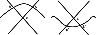
     Figure 5: The third Reidemeister move and corresponding crossings

     We require that

     a) $p(x)=p(x^{\prime}),p(y)=p(y^{\prime}),p(z)=p(z^{\prime})$;

     b) Among $x,y,z$, the number of odd crossings is even (i.e., is equal to $0$ or $2$).

  4. For every Reidemeister move $K_{1}\to K_{2}$ there exists a one-to-one correspondence between crossings of $K_{1}$ away from the Reidemeister move, and crossings of $K_{2}$ away from the Reidemeister move.

     We require that the corresponding crossings of the diagrams $K_{1}$ and $K_{2}$ are of the same parity.

We introduce the notion of justified parity analogously to the notion of parity.

• 4. By justified parity of crossings we mean a parity where each odd crossing is marked by a letter $b$ or $b^{\prime}$ (in these cases we call a crossing an odd crossing of the first type or an odd crossing of the second type, respectively), so that the following holds:

  1. If a second Reidemeister move is applied to two odd crossings then they are of the same type (either both are $b$ or both are $b^{\prime}$).

  2. If in a third Reidemeister move we have two odd crossings, then each of them changes its type after the Reidemeister move is applied (the crossing marked by $b$ before the Reidemeister move is applied should correspond to the crossing marked by $b^{\prime}$ after the Reidemeister move is applied).

  3. Moreover, odd crossings not taking part in the Reidemeister move, do not change their types.

We define the Gaussian parity and the Gaussian justified parity on framed $4$-graphs with one unicursal component, as follows.

• 5.[The Gaussian parity and justified parity] Let $D$ be a chord diagram.

  We say that a chord of $D$ is even (after Gauss), if the number of chords linked with it, is even, and odd, otherwise. Furthermore, an odd chord is of the first type if it is linked with an even number of even chords; otherwise an odd chord is said to be of the second type (after Gauss).

  For a framed $4$-graph $\Gamma$ corresponding to a chord diagram $D$ the Gaussian parity and justified parity are defined as those of the corresponding chord diagram.

It can be easily checked that the Gaussian parity and the Gaussian justified parity satisfy the axioms of parity and justified parity.

Later in this paper, for cobordism purposes we shall then extend the notion of Gaussian parity and justified Gaussian parity for another situation. To that end, we shall first define the Gaussian parity for double lines of a $2$-disc with generic intersections, and then for every regular section of this disc (which will be a framed $4$-graph representing a free link) we shall define the parity for crossings to be the parity of double lines it comes from.

However, for the first goal (the construction of an invariant of free knots) it would be sufficient for us to have a well defined parity just for framed $4$-graphs with one unicursal component.

1.4 A functorial mapping $f$

Let $K$ be a framed $4$-graph. Let $f$ be a diagram obtained from $K$ by removing all odd crossings and connecting opposite edges of former crossings to one edge.

Theorem 1.

The map $f$ is a well-defined map on the set of all free knots. For a virtual knot diagram $K$, $f(K)=K$ iff all crossings of $K$ are even. Otherwise, the number of classical crossings of $f(K)$ is strictly less than the number of classical crossings of $K$.

This theorem was known to Turaev for the case of Gaussian parity; in the general case it easily follows from the parity axioms.

As we shall see, this map will take slice free knots to slice free knots and will never increase the slice genus.

2 An invariant of free knots

In the present section, we shall construct an invariant of free knots constructed from the parity and justified parity, and prove its invariance. We shall later prove that this invariant delivers a sliceness obstruction for a free knot. Within the present section, by parity and justified parity we mean the Gaussian parity and the Gaussian justified parity.

An extension of the invariant to be presented below, is constructed in [10]; for our purposes (sliceness obstruction) the version given here will suffice, nevertheless, it is an important question to investigate the invariant from [10] related to the sliceness.

Set $G=\langle a,b,b^{\prime}|a^{2}=b^{2}=b^{\prime 2}=e,ab=b^{\prime}a\rangle$.

Our first goal is to construct an invariant of free long knots (resp., of compact free knots) valued in $G$ (in the set of conjugacy classes of the group $G$).

Let $D$ be an oriented chord diagram, with a marked point $X$ on the core circle $C$ distinct from any chord end. Later we shall see how one can get rid of the orientation of $D$.

We distinguish between even and odd chords of $D$; moreover, we distinguish between two types of odd chords of $D$.

With a marked oriented chord diagram $(D,X)$ we associate a word in the alphabet $\{a,b,b^{\prime}\}$, as follows. Let us walk along the core circle $C$ of the diagram $D$ starting from $X$. Every time we meet a chord end, we write down a letter $a,b$ or $b^{\prime}$ depending on whether the chord whose endpoint we met, is even, first type odd, or second type odd. Having returned to the point $X$, we obtain a word $\gamma(D,X)$; this word determines an element of $G$; by abuse of notation we shall denote this element by $\gamma(D,X)$ as well. Moreover, sometimes we shall omit $X$ from the notation when it is clear from the context which initial point we have chosen.

Theorem 2.

If two marked chord diagrams $(D,X)$ and $(D^{\prime},X^{\prime})$ generate equivalent free knots then the following two conjugacy classes coincide: $[\gamma(D)]=[\gamma(D^{\prime})]$ in $G$.

An extended version of this theorem is proved in [10]; see also

Proof.

Indeed, if $D$ and $D^{\prime}$ differ by one first Reidemeister move (say, $D^{\prime}$ has one extra chord) then the word $\gamma(D^{\prime})$ is obtained from $\gamma(D)$ by an addition of two consequent letters $a\cdot a$; thus, the corresponding elements from $G$ coincide.

Analogously, if $D^{\prime}$ obtained from $D$ by an increasing second Reidemeister move, then the two new chords of $D^{\prime}$ are of the same parity and of the same type; denote the letter corresponding to each of these two chords ($a$,$b$ or $b^{\prime}$), by $u$. Thus, the word $\gamma(D^{\prime},X^{\prime})$ is obtained from $\gamma(D,X)$ by addition of $u\cdot u$ in two places. As in the first case, it does not change the corresponding element of $G$.

When applying the third Reidemeister move $D\to D^{\prime}$ one of the following two possibilities may occur. In the first case, all three chords participating in the third Reidemeister move, are even.

In this case the words $\gamma(D)$ and $\gamma(D^{\prime})$ coincide identically.

In the second case, two of the three chords taking part in the Reidemeister move, are odd, and one chord is even. Consider those three segments of the words $\gamma(D)$ and $\gamma(D^{\prime})$ where the ends of the three moving chords are located. For those segments containing an end of the odd chord, we get one of the two substitutions $ab\longleftrightarrow b^{\prime}a$ or $ba\longleftrightarrow ab^{\prime}$: indeed, after the third Reidemiester move, the odd chord has changed its type.

Both changes correspond to some relations in $G$.

Now consider the segment of the diagram containing the two ends of the odd chords. If these two odd chords are of the same type in $D$, then in $D^{\prime}$ they are of the same type as well. Consequenlty, when passing from $\gamma(D)$ to $\gamma(D^{\prime})$ we replace the subword $b\cdot b$ by $b^{\prime}\cdot b^{\prime}$ or vice versa. Since both subwords correspond to the trivial element of $G$, we have $\gamma(D)=\gamma(D^{\prime})$ in $G$.

Finally, if the two chords participating in the third Reidemeister move, are of different types on the diagram $D$, then when passing from $\gamma(D)$ to $\gamma(D^{\prime})$ the order of $b$, $b^{\prime}$ in the fragment of the corresponding word stays the same: the adjacent letters $b$ and $b^{\prime}$ change their position twice.

Thus, no Reidemeister move changes the element of $G$ corresponding to the chord diagram. ∎

This theorem immediately yields the following

Corollary 1.

The conjugacy class of the element $[\gamma(D,X)]$ in $G$ is an invariant of free knots given by the diagram $D$, i.e., it does not depend on the fixed point $X$.

Indeed, moving the marked point through a chord end corresponds to a cyclic permutation of the letters, which, in turn, generates a conjugation in $G$.

2.1 The Cayley graph of $G$

Its Cayley graph looks like a vertical strip on a squared paper between $x=0$ and $x=1$: we choose the point $(0,0)$ to be the unit in the group; the multiplication by $a$ on the right is chosen to be one step in a horizontal direction (to the right if the first coordinate of the point is equal to zero, and to the left if this first coordinate is equal to one), the multiplication by $b$ is one step upwards if the sum of coordinates is even and one step downwards if this sum is odd, and the multiplication by $b^{\prime}$ is one step downwards if the sum of coordinates is even and one step upwards if the sum of coordinates is even, see Fig. 6.

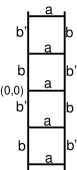
Figure 6: The Cayley graph of the group $G$

With each pointed chord diagram one associates an element from $G$ having coordinates $(0,l)$. Moreover, the conjugacy class of the element $(0,l)$ for $l\neq 0$ consists of the two elements: $(0,4l)$ and $(0,-l)$. Thus, for each long free knot one gets an integer-valued invariant, equal to $l$; we shall denote this invariant by $l(K)$; each compact free knot has, in turn, the invariant equal to $|l|$; we shall denote the latter by $L(K)$.

It is an easy exercise to show that $l$ is divisible by $4$; in fact, it can be also shown that $l$ is divisible by $8$.

It is obvious that if we invert the orientation of the chord diagram, we shall reverse the order of letters in the word $\gamma$; this leads to the switch $(0,l)\to(0,-l)$. So, the invariant $L(K)$ can be defined for unoriented free knots.

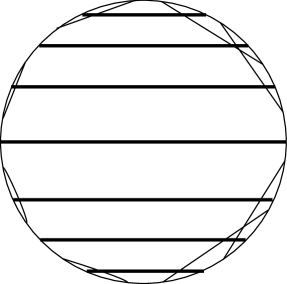
Figure 7: A non-slice free knot

We shall describe elements of $G$ by two coordinates on the Cayley graph. It can be easily checked that any element of $G$ corresponding to a chord diagram has coordinates $(0,4m)$. Indeed, the word corresponding to a Gauss diagram has an even number of occurences of $a$, and the total number of letters $b$ and $b^{\prime}$ is divisible by four. The latter, in turn, follows from the fact that the number of odd chords of a chord diagram is even, which, in turn, just means that the number of odd-valent vertices of any graph is always even. Moreover, the conjugacy class of the element with coordinates $(0,4m)$, $m\neq 0$ in $G$ consists of two elements: $(0,4m)$ and $(0,-4m)$. Thus, every compact free knot has an integer-valued invariant equal to $L=|4m|$ (it will be convenient for us to preserve the factor $4$ in the definition of our invariant).

In Fig. 7 we have a free knot $K_{1}$ for which $L(K_{1})=16$.

We use bold lines to describe even chords. The corresponding word in $G$ (with an appropriate choice of the marked point) looks like $(b^{\prime}a)^{7}b^{\prime}b(ab)^{7}=(b^{\prime}b)^{16}$.

2.2 Remarks on the definition of the invariant $L$ for links

Note that Theorem 2 works for any parity, not only for the Gaussian one.

For cobordism purposes, we have to understand the behaviour of the invariant $L$ not only under Reidemeister moves, but also under Morse bifurcations.

Our further strategy is as follows. Assuming we have a cobordism (see Definition 4) ${\cal D}\to D$ that spans the curve $\gamma$, we shall define the parity and justified parity of double lines (i.e., those lines on $D$ having preimages consisting of two connected components). This parity will be defined in a way such that the parity (the justified parity) for a double point on $\gamma$ will coincide with the parity (justified parity) for a double line, this point belongs to. Besides, this approach will allow us to define the parity and the justified parity for any generic section of a cobordism; such a section will be a framed $4$-graph representing a multicomponent link. With these parity and justified parity in hand, we shall be able to extend our invariant $L$ to sections of $L$ (levels of the Morse function on $D$) and then understand the behaviour of this invariant under Morse bifurcations.

For a single component free-link (free knot), the value of the invariant $\gamma$ can be expressed by one non-negative integer $L$. For a cobordism, every section is a multicomponent free link, so, we have to define the invariant $\gamma$ on this multicomponent link to be a collection of conjugacy classes of elements of $G$ (one for each component), and we may require that these elements of $G$ are expreseed by one non-negative integer number each, in order to associate an integer number to each component.

To this end, we shall need that:

1) The parity and the relative parity are well-defined for sections and well-behaved under Morse moves.

2) The number of even intersection points on each component is even; otherwise the corresponding element of $G$ will have a non-zero first coordinate.

3) The value of the first coordinate of the element of $G$ (described by the invariant $L$) behaves well with respect to any Morse bifurcations.

In particular, every component of a non-singular level link has an even number of intersection points: it is necessary to describe the value of our invariant $L$ for the parity to be well defined. Indeed, in order to define the Gaussian parity of some crossing, one has to take some “half” of the circle corresponding to this crossing and count the number of intersection points belonging to this half. In the case of a free knot the parity of this number of points does not depend on the half one chooses because it equals the parity of the number of chords linked with the chord in question.

When we have a two-component link, and we take a crossings formed by single component, the two parities corresponding to the two halves will be different if the total number of crossings between components is odd.

So, for those $2$-component links having an odd number of intersection points between components, there is no immediate way to extend the Gaussian parity.

As we shall see further, all these conditions will be automatically satisfied when we consider the sections of a disc cobordism.

3 Parity as homology

In the present section, we are going to reformulate the notion of parity and justified parity in terms of homology, [8]. This reformulation will be useful for understanding the way how to define the parity on double lines of the cobordism.

Consider a framed $4$-graph $\Gamma$ with one unicursal component. The homology group $H_{1}(\Gamma,{\mathbb{Z}}_{2})$ is generated by “halves” corresponding to vertices: for every vertex $v$ we have two halves of the graph $\Gamma_{v,1}$ and $\Gamma_{v,2}$, obtained by smoothing at this vertex, see Fig. 8. If the set of all framed $4$-graphs (possibly, with some further decorations at vertices) is endowed with a parity, we may assume that we are given the following cohomology class $h$: for each of the halves $\Gamma_{v,1},\Gamma_{v,2}$ we set $h(\Gamma_{v,1})=h(\Gamma_{v,2})=p(v)$, where $p(v)$ is the parity of the vertex $v$. Taking into account that every two halves sum up to give the cycle generated by the whole graph, we have defined a “characteristic” cohomology class $h$ from $H^{1}(\Gamma,{\mathbb{Z}}_{2})$.

Let $c\in H_{1}(\Gamma,{\mathbb{Z}}_{2})$ be a subgraph of $\Gamma$. Denote by $d(c)$ the collection of those vertices of $\Gamma$ where $c$ is incident to exactly two half-edges, and these two edges are non-opposite.

Then it follows immediately that $c$ is equal to the sum $\sum_{i}\Gamma_{d_{i},1}$ up to an overall addition of $\Gamma$.

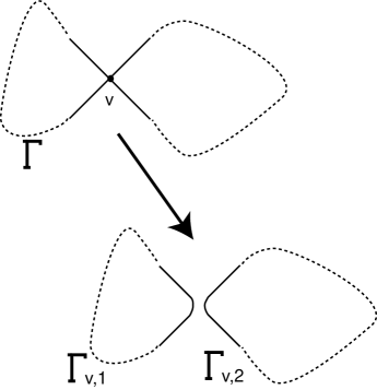
Figure 8: The halves $\Gamma_{v,1}$ and $\Gamma_{v,2}$

Collecting the properties of this cohomology class and recalling the parity axiomatics, we see that

1. For every framed $4$-graph $\Gamma$ we have $h(\Gamma)=0$.

2. If $\Gamma^{\prime}$ is obtained from $\Gamma$ by a first Reidemeister move adding a loop then for every basis $\{\alpha_{i}\}$ of $H_{1}(\Gamma,{\mathbb{Z}}_{2})$ there exists a basis of the group $H_{1}(\Gamma,{\mathbb{Z}}_{2})$ consisting of one element $\beta$ corresponding to the loop and a set of elements $\alpha^{\prime}_{i}$ naturally corresponding to $\alpha_{i}$.

   Then we have $h(\beta)=0$ and $h(\alpha_{i})=h(\alpha^{\prime}_{i})$.

3. Let $\Gamma^{\prime}$ be obtained from $\Gamma$ by a second increasing Reidemeister move. Then for every basis $\{\alpha_{i}\}$ of $H_{1}(\Gamma,{\mathbb{Z}}_{2})$ there exists a basis in $H_{1}(\Gamma^{\prime},{\mathbb{Z}}_{2})$ consisting of one “bigon” $\gamma$, the elements $\alpha^{\prime}_{i}$ naturally corresponding to $\alpha_{i}$ and one additional element $\delta$, see Fig. 9, left.

   

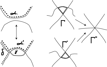
   Figure 9: The cohomology condition for Reidemeister moves

   Then the following holds: $h(\alpha_{i})=h(\alpha^{\prime}_{i})$, $h(\gamma)=0$.

   (note that we impose no constraints on $\delta$).

4. Let $\Gamma^{\prime}$ be obtained from $\Gamma$ by a third Reidemeister move. Then there exists a graph $\Gamma^{\prime\prime}$ with one vertex of valency $6$ and the other vertices of valency $4$ which is obtained from either of $\Gamma$ or $\Gamma^{\prime}$ by contracting the “small” triangle to the point. This generates the mappings $i:H_{1}(\Gamma,{\mathbb{Z}}_{2})\to H_{1}(\Gamma^{\prime\prime},{\mathbb{Z}}_{2})$ and $i^{\prime}:H_{1}(\Gamma^{\prime},{\mathbb{Z}}_{2})\to H_{1}(\Gamma^{\prime\prime},{\mathbb{Z}}_{2})$, see Fig. 9, right.

   Then the following holds: the cocycle $h$ is equal to zero for small triangles, besides that if for $a\in H_{1}(\Gamma,{\mathbb{Z}}_{2}),a^{\prime}\in H_{1}(\Gamma^{\prime},{\mathbb{Z}}_{2})$ we have $i(a)=i^{\prime}(a^{\prime})$, then $h(a)=h(a^{\prime})$.

Thus, every parity for free knots generates some ${\mathbb{Z}}_{2}$-cohomology class for all framed $4$-graphs with one unicursal component, and this class behaves nicely under Reidemeister moves.

The converse is true as well. Assume we are given a certain “universal” ${\mathbb{Z}}_{2}$-cohomology class for all four-valent framed graphs satisfying the conditions 1)-4) described above. Then it originates from some parity. Indeed, it is sufficient to define the parity of every vertex to be the parity of the corresponding half. The choice of a particular half does not matter, since the value of the cohomology class on the whole graph is zero. One can easily check that parity axioms follow.

This point of view allows to find parities for those knots lying in ${\mathbb{Z}}_{2}$-homologically nontrivial manifolds.

4 Slice Genus and Cobordisms of Free Knots

• 1. Let $K$ be a framed $4$-valent graph. We say that $K$ has slice genus at most $h$ if there exists a surface ${\cal D}_{h}$ of genus $h$ with one boundary component $S$, a $2$-complex $D_{h}\supset K$, and a continuous map $g:{\cal D}_{h}\to D_{h}$, such that:

  1. $g(\partial{\cal D}_{h})=K\subset D_{h}$; for every vertex $v$ of $K$ we have $g^{-1}(v)=\{v_{1},v_{2}\}$, and small neighbourhood $U(v_{1})\subset S$ is mapped to a pair of opposite edges of $K$ at $v$;

  2. the map $g$ is one-to-one everywhere except on the union of intervals: $\Sigma=\{x\in D_{h}:Card(g^{-1}(x))>1\}$;

  3. the subset $\Sigma_{3}=\{x\in D_{h}:Card(g^{-1}(x))>2\}$ is finite, and consists only of those points having exactly three preimages; moreover $\Sigma_{3}\cap{\partial D}_{h}=\emptyset$; double lines (preimages of $\Sigma\backslash\Sigma_{3}$ approach $\partial{\cal D}_{h}$ transversally.

The surface ${\cal D}_{h}$ will be called the spanning surface or the cobordism of genus $h$.

In other words, we require that the free knot $K$ (image of the circle $S$) is spanned by $D_{h}$, image of the $2$-surface ${\cal D}_{h}$ with boundary $S$ and the singularities of the map $g:{\cal D}_{h}\to D_{h}$ are all generic.

Analogously, one defines the cobordism of genus $h$ for graph-links.

The relation $\sim$ for free-knots to be cobordant is defined for cobordisms of genus $0$.

The closure ${\bar{\Sigma}}$ contains also cusps: those points $x\in D_{h}$ for which $Card(g^{-1}(x))=1$ and such that for every small neighbourhood $U(x)$, the intersection $U(x)\cap\Sigma$ is the punctured interval. Let $\zeta=g(\partial{\cal D})$. Denote by $\Psi$ the preimage $g^{-1}(\bar{\Sigma})\subset{\cal D}_{h})$. Let $\Sigma_{2}$ be $\Sigma\backslash\Sigma_{3}$.

The image $g(S)\subset D_{h}$ is a four-valent framed graph in $D_{h}$. Indeed, this image is obtained from $S=\partial{\cal D}_{h}$ by gluing double points of $S$; it has the framing (opposite edge structure) induced from $S$: for a point $x$ in $g(S)\cap\Sigma$, the preimage $g^{-1}(U(x)\cap g(S))$ consists of two branches of $S$; the images of those two branches will generate the two pairs of opposite edges.

• 2. If $K$ admits a cobordism of genus $h$ and does not admit a cobordism of genus $h-1$ we say that $K$ has slice genus $h$. Notation: $sg(K)=h$.

  A free knot of genus $0$ is called null-cobordant or slice.

The following lemma follows from the definition of free knot:

Lemma 1.

If framed $4$-graphs $K,K^{\prime}$ represent equivalent free knots then $K$ and $K^{\prime}$ are cobordant and $sg(K)=sg(K^{\prime})$.

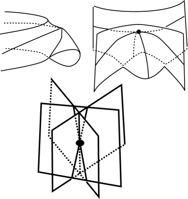
Figure 14: Elementary cobordisms for Reidemeister moves

Indeed, in Fig. 14 we demonstrate the cobordisms between $K$ and $K^{\prime}$: the first Reidemeister move corresponds to a cusp point, the second Reidemeister move corresponds to a passage through a tangency point, and the third Reidemeister move corresponds to a triple point

Thus, it makes sense to speak about the slice genus of free knots.

• 3. Let $K$ be a flat virtual knot and $|K|$ be the underlying free knot. Then it follows from the definition that the slice genus of $K$ is greater than or equal to the slice genus of $|K|$. In particular, if $K$ is slice then so is $|K|$.

Example 1.

The first example of a non-slice flat virtual knot was constructed by Carter [2], it is shown in Fig. 10.

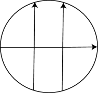
Figure 10: Carter’s non-slice flat virtual knot

In Fig. 10, the arrows indicate the clockwise direction of branches. Namely, orient the core circle of the chord diagram counterclockwise and orient the immersed curve accordingly. If two oriented branches $(a,b)$ of the curve have an intersection at a double point $X$ and the tangent vectors $v_{X,a},v_{X,b}$ form a positively-oriented basis, then the arrow is directed from $a$ to $b$.

In this notation, for flat virtual knots, two chords pariticipating in a second Reidemeister move should have opposite orientations. The flat knot in Fig. 10 is non-trivial as a flat virtual knot. Nevertheless, when we forget about the arrows and pass to the free knot, we can first cancel the two vertical arrows (by a second Reidemeister move) and then cancel the horizontal arrow (by a first Reidemeister move). So, the corresponding free knot $|K|$ is trivial, and hence slice.

So, if a free knot is non-slice, then so is every flat virtual knot corresponding to it. The problem of finding non-slice free knots is rather complicated. Another definition of cobordisms (having another meaning), is given in [4] (it follows Turaev’s definition for cobordisms of words [12]). In this paper, two free knots are called cobordant if one can be obtained from the other by a sequence of combinatorial moves. Some invariants of such cobordisms are constructed, and non-sliceness of knots is proved. We shall investigate the relation between those combinatorial cobordisms and topological cobordisms studied in the present paper, in a consequent paper.

In the work of Carter [2] and Turaev [12], topological sliceness obstructions for immersed curves were studied: for each double point $x$ of an immersed curve $\Gamma$, one considers the homology class of the halves $\Gamma_{x,1}$ for different vertices $x$, and takes the homological pairing of these halves in the surface. This approach can not be applied to free knots because a framed four-valent graph is not assumed to be embedded in any $2$-surface. Moreover, embeddings into different $2$-surfaces may crucially change the intersection form for “halves” even with ${\mathbb{Z}}_{2}$-coefficients.

5 Parity of Curves in $2$-surfaces

Let us now pay more attention to the structure of cobordisms of free knots. Assume there is a cobordism $g:{\cal D}\to D$ (of genus zero) spanning the free knot $K=g(\partial D)$.

Set $\Psi=g^{-1}({\bar{\Sigma}})$. Then $\Psi$ has a natural stratification containing strata of dimensions zero and one. The strata of dimension $0$ are double points on the boundary, cusps, and triple points. By a double line we mean a minimal (with respect to inclusion) collection of $1$-dimensional strata possessing the following properties:

1) two strata attaching the same cusp belong to the same double line;

2) two strata attaching the same triple point from opposite sides belong to the same double line, see Fig. 11.

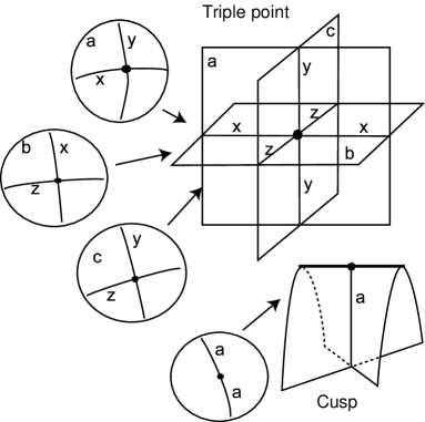
Figure 11: Double lines $a,x,y,z$,cusps and triple points

Let $x\in K\cap\Sigma$ be a double point on the boundary of $\partial D$. Assume $g^{-1}(x)=\{x_{1},x_{2}\}$.

Recall the definition of the Gaussian parity for a vertex $x$ of the framed graph: we take an arc ${\iota}$ of $K$ connecting $x$ to $x$, being the image of an arc ${\tilde{\iota}}$ on $S$, and count the parity of the double point number on ${\iota}$.

Now, let us consider the preimage ${\tilde{\iota}}\subset S$ connecting $x_{1}$ to $x_{2}$. Then $p(x)$ can be reformulated as the parity of the set $Card(\tilde{\iota}\cap\Sigma)$. Note that this line ${\tilde{\iota}}$ belongs to the boundary of the disc ${\cal D}$.

Note that in this definition we may choose ${\iota}$ to be any of the two halves of the circle, and the resulting parity will not depend on that choice. Moreover, we take a path from $x_{1}$ to $x_{2}$ locally directed towards the same half at both points, and count the number of double points inside it.

Thus, instead of ${\tilde{\iota}}\subset{\partial{\cal D}}$ we may take an arbitrary path $\eta\subset{\cal D}$ in generic position to ${\bar{\Sigma}}$ connecting $x_{1}$ to $x_{2}$: we assume that $\eta\cap{\bar{\Sigma}}=\eta\cap\Sigma_{2}$ consists only of transverse intersections. All such curves lie on a disc ${\cal D}$ and have the same fixed ends, so they are all homotopic (rel. boundary) to each other. The only thing we have to fix is the behaviour of the curve in the neighbourhood of $x_{1}$ and $x_{2}$. When we take ${\tilde{\eta}}\subset{\cal D}$, then the neighbourhoods ${\tilde{\eta}}\cap U(x_{1})$ and ${\tilde{\eta}}\cap U(x_{2})$ belong to the same half of the circle $S$. In terms of ${\cal D}$ and $D$, this can be reformulated as follows.

Let $\zeta\subset D$ be the $1$-stratum in $D$ attaching the point $x$. Orient $\zeta$ arbitrarily, and orient the two preimages $\zeta_{1}\cap U(x_{1})$ and $\zeta_{2}\cap U(x_{2})$ accordingly. Consider the two vectors $v_{1}$ and $v_{2}$ tangent to ${\tilde{\iota}}$ at $x_{1}$ and $x_{2}$. We require that the bases $({\dot{\zeta}_{1}},v_{1})$ and $({\dot{\zeta}_{2}},v_{2})$ generate two different orientations of the disc ${\cal D}$. If we change the direction of both $x_{1}$ and $x_{2}$ it will not change the parity of ${\tilde{\iota}}\cap\Sigma_{2}$; here ${\dot{\zeta}_{i}}$ stays for the unit tangent vector to $\zeta_{i}$, see Fig. 12.

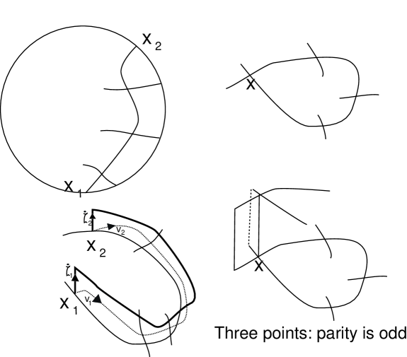
Figure 12: The geometric way for defining parity

So, this gives another way to define a parity for $x$. Consider it as the defintion of any double point.

Now, we can do the same for any arbitrary point on the double line $x$. We call it the Gaussian parity of a vertex $x$.

The following Statement easily follows from the definition:

Statement 1.

The Gaussian parity is constant along double lines.

Proof.

This is evident for two points belonging to the same $1$-stratum and for points on two strata attaching the same cusp. When passing through a triple point, the parity does not change, see Fig. 13. We see that the curve connecting the two preimages of $A$ is parallel to the curve connecting the two preimages of $B$ everywhere except for the two small domains; inside these two domains, we have two intersections with double lines $p$ and $q$ which cancel each other. ∎

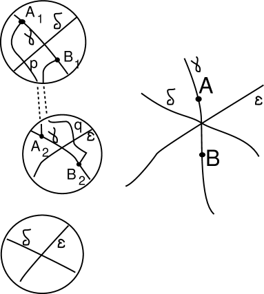
Figure 13: The behaviour of parity and justified parity when passing through a triple point

This leads to the definition of parity for a double line:

• 1. Take an arbitrary generic (non-triple and not a cusp) point $x$ on a double line $\gamma$, and consider the two preimages $x_{1}$ and $x_{2}$ of it on ${\cal D}$. Connect $x_{1}$ to $x_{2}$ by a generic path ${\tilde{\eta}}$, such that the behaviour of $\gamma$ in neighbourhoods $U(x_{1})$ and $U(x_{2})$ is coordinated (as in the definition of Gaussian parity). Now, the Gaussian parity of the double line containing $x$ is the parity of the number of intersection points between ${\tilde{\eta}}$ and $\Psi$.

This allows to define the set $\Psi_{even}$ to consist of all those points of $\Psi$ beloning to even double lines.

Now, to define the justified Gaussian parity, we should take an odd double line $\gamma$, an arbitrary generic point $x$ on it, and consider the two preimages $x_{1}$ and $x_{2}$ of $x$. Then we connect $x_{1}$ to $x_{2}$ by a generic path $\delta\in{\cal D}$ and count the number of intersections between $\delta$ and $\Psi_{even}$. If this number is even, we say that the $1$-stratum of the odd double line containing $x$ is of the first type; otherwise we say that this $1$-stratum is of the second type. Note that the definition of type is even easier than the definition of parity: we should not care about the local directions at the endpoints since we do not count the number of intersections with odd lines.

One immediately gets the following

Statement 2.

The Gaussian justified parity is constant on $1$-strata belonging to $\Psi$. It changes from $b$ to $b^{\prime}$ or from $b^{\prime}$ to $b$ when passing through a triple point formed by two odd double lines and one even double line.

Proof.

The invariance along $1$-stratum is evident. Now view Fig. 13. Assume the double $\gamma$ and $\delta$ are odd and the line $\epsilon$ is even. Then the two lines connecting the preimages of $A$ and the preimages of $B$ are “parallel” except for two domains where one of them passes through a double line at $p$, and the other one passes through a double line at $q$. Since we disregard intersection with odd double lines, we see that $q$ counts and $p$ does not. ∎

Having defined the Gaussian parity and Gaussian justified parity in this way, we will be able to construct the invariant $L$ for any section of a cobordism $D$.

6 Sliceness of Free Knots. The Main Theorem

It turns out that the invariant $L$ of free knots is an obstruction to slicness.

Before proving the main statement, we shall make several observations concerning sliceness. By Lemma 1, it follows that the slice genus is well defined on the set of free knots.

The following statement is trivial.

Statement 3.

If a framed $4$-graph $K^{\prime}$ is equivalent to a framed $4$-graph $K$ (by Reidemeister moves), then the slice genus of $K^{\prime}$ is equal to that of $K$. In particular, if $K$ is slice then so is $K^{\prime}$.

Thus, it makes sense to talk about cobordisms of free knots, not merely about cobordisms of framed $4$-graph.

As a corollary, we get the following

Statement 4.

If a framed $4$-graph $K$ is embeddable in $S^{2}$ or $T^{2}$ then $K$ is slice.

Indeed, every framed $4$-graph on $S^{2}$ is equivalent (as a flat knot) to the flat unknot; every framed $4$-graph on $T^{2}$ is homotopic either to the trivial loop on the torus (with no crossings) or to a non-separating loop without crossings (one may think of such a loop as the longitude or the meridian in some coordinate system), so, it is an unknot as well. Consequently, all such knots are trivial in the free knot category.

Statement 5.

Let $K$ be a free knot, and let ${{\cal F}}(K)$ be a free knot obtained from $K$ by deleting odd crossings. If $K$ is slice then so is ${\cal F}(K)$.

Proof.

Indeed, any cobordism for $K$ generates a cobordism for ${\cal F}(K)$ obtained by separating all odd double lines: two points from $\Sigma_{2}$ will be pasted together only if they lie on an even double line. Note that this makes no contradiction with triple points: a triple point either survives if it belongs to three even double lines, or one sheet becomes disjoint from the two other ones if two of the three double lines are odd. ∎

Denote the obtained cobordism for ${\cal F}(K)$ by ${\cal F}(D)$.

The main result of the present paper is the following

Theorem 3 (Main Theorem).

If a free knot $K$ has $L(K)\neq 0$, then $K$ is not slice.

In particular, this yields the following

Corollary 2.

Let $\gamma$ be a curve immersed in an oriented closed $2$-surface $S_{g}$. Then if for a free knot $\Gamma$ corresponding to $\gamma$ one has $L(\Gamma)\neq 0$ then the underlying $\gamma$ is not slice as a flat virtual knot.

Indeed, a general position image of the disc in a $3$-manifold is a spanning disc having only three-dimensional singularities. The converse statement is, generally, not true.

The problem of finding obstructs for a surface $S_{g}$ with a curve $\gamma$ to span a disc immersed in a $3$-manifold was studied by Carter [2], Turaev, [12] etc. Some topological obstructions based on homology of $S_{g}$ were constructed.

In the present paper we consider a more complicated problem: instead of curves in $2$-surfaces we consider framed four-valent graphs, and instead of spanning $2$-discs in $3$-manifolds we consider “abstract” spanning $2$-discs. However, as we see from the above discussion concerning parity and homology and the formulation of the main theorem, the notion of parity which plays the role of “subsitute of homology of $S_{g}$”.

6.1 Constructing the Morse function and the Reeb graph

The proof will consist of several steps.

We shall adopt the following notation for the maps: by $g$ we shall mean the map ${\cal D}\to D$ corresponding to the cobordism, and by $f$ we shall denote either of the two maps: the Morse function $f:D\to{\mathbb{R}}$ (see definition ahead) and the composition $g\circ f:{\cal D}\to{\mathbb{R}}$ will be also denoted by $f$ (abusing notation).

Assume the knot $K$ is slice and admits a cobordism $g:{\cal D}\to D$ (of genus zero).

• 1. By a Morse function on $D$ we mean a Morse function $f:{\cal D}\to[0,\infty)$ such that if $g(x)=g(y)$ then $f(x)=f(y)$, all Reidemeister move points: triple points, cusp points and tangency points on ${\cal D}$, lie on non-critical levels of $f$, and $f^{-1}(0)=K,f^{-1}(1)=\emptyset$. By abuse of notation we shall denote the function on ${\cal D}$ and the function on $D$ by the same letter $f$. By a non-singular value of the function $f$ we mean a noncritical value $X$ such that $f^{-1}(X)\subset{\cal D}$ contains no cusps and no triple points. A Morse function on $D$ will be called simple if every singular level contains either exactly one critical point or exactly one triple point or exactly one cusp point.

From now on, we require that the Morse function of $D$ is simple and the level $0$ is non-singular. It is clear that such Morse functions are everywhere dense in the class of all functions. Every Morse function has singular levels of two types: those corresponding to Morse bifurcations (saddles, minima, and maxima) and those corresponding to Reidemeister moves (corresponding to cusps, tangency points and triple points). Denote singular levels of the function $f$ by $c_{1}<\dots<c_{k}$ and choose non-critical levels $a_{i}$: $0=a_{0}<c_{1}<a_{1}<c_{2}<\dots a_{k}<c_{k}<a_{k+1}=1$.

Let us construct the Reeb graph $\Gamma_{f}$ (molecula) of the function $f$ as follows. The univalent vertices of the Reeb graph will correspond to minima and maxima of the function $f$; the vertices of valency three will correspond to saddle points; edges will connect critical points; every edge will correspond to a cylinder $S^{1}\times I\subset{\cal D}$ which is continuously mapped by $f$ to a closed interval between some two critical point; this cylinder has no Morse critical points inside. One edge will emanate from the point $0$ corresponding to the circle $S=\partial{\cal D}$, see Fig. 15.

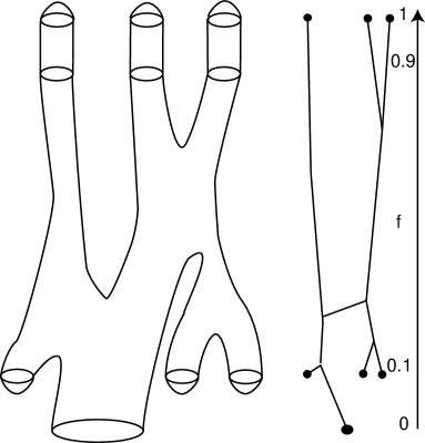
Figure 15: The Reeb graph and circle bifurcations

Since this graph is a Reeb graph of the Morse function on a disc ${\cal D}$, the graph $\Gamma_{f}$ is a tree.

Our next goal is to endow each edge of the Reeb graph with a non-negative integer label. The label of the edge emanating from $0$ will coincide with $L(K)$.

For every non-singular level $c$ of $f$ the preimage $K_{c}=f^{-1}(c)\subset D$ is a free link; when passing through a Reidemeister singular point, the link $K_{c}$ is operated on by the corresponding Reidemeister move; when passing through a Morse critical point it gets operated on by a Morse-type bifurcation. Every crossing of $K_{c}$ belongs to some double line of $D$. Define the parity of the crossing to be the Gaussian parity of the double line, it belongs to. Analogously, define the justified parity of a crossing to be that of the stratum it belongs to. One can easily see that if a section of the Morse function is a framed $4$-valent graph with one unicursal component then the parity and justified parity coincide with the Gaussian parity and justified parity defined directly via Gauss diagram.

Consider the free link $K_{c}$ and orient its components arbitrarily (as we shall see further, the orientation will be immaterial); for every unicursal component $K_{c,j}$ of the free link $K_{c}$ we may define the conjugacy class $\delta(K_{c,j})$ of $\gamma(K_{c,j})$ in $G$ just as it is done for free knots with Gaussian parity and justified parity. Let $\delta(K_{c})$ be the unordered collection of all $\delta(K_{c,j})$ for all $j$ (with repetitions).

From Statements 1 and 2 we get the following

Lemma 2.

The parity and justified parity defined on the set of $K_{c}$ satisfy the parity and justified parity axioms under those Reidemeister moves which happen within the cobordism $D$.

This lemma, in turn, yields the following

Lemma 3.

For an interval $[a,b]\subset[0,1]$ containing Reidemeister singular points and no Morse critical points (for a coordinated choice of orientations of link components) we have $\delta(K_{a})=\delta(K_{b})$ as collections of conjugacy classes of elements from $G$ counted with multiplicities.

Moreover, $\delta(K_{0})$ is the conjugacy class of $\gamma(K)$.

The proof literally repeats the proof of Theorem 2 applied to each unicursal component of the link.

Now, we would like to treat $\delta$ as a collection of non-negative integers rather than just conjugacy classes and to forget about orientations of components of $K_{c}$. To this end, we prove the following

Lemma 4.

Let $c$ be a non-singular level of $f$, and let $K_{c,1},\dots,K_{c,n}$ be unicursal components of the free link $K_{c}=f^{-1}(c)\subset D$. Then for every $i=1,\dots,n$:

1) The total number of intersection points between $K_{c,i}$ and $K_{c,j},j\neq i$, is even.

2) The number of odd intersection points between $K_{c,i}$ and $K_{c,j},j\neq i$, is even.

Proof.

The proof follows from the fact that the preimage of $K_{c,i}$ in ${\cal D}$ is a circle, and the intersection of a closed circle with a set $\Psi$ (or $\Psi_{even}$) in ${\cal D}$ consists of an even number of points. ∎

Lemma 4 immediately yields that every $\gamma(K_{c,i})$ for a non-singular $c$ is represented by an element $(0,l)$ on the Cayley graph of $G$.

Let $L_{c}=\{l_{c,1},\dots,l_{c,m}\}$ be the collection of integers (with repetitions) obtained from $\delta(K,c)$ by replacing conjugacy classes with absolute values of their second coordinates.

Each $l_{c,i}\in{\mathbb{N}}\cup\{0\}$ corresponds to a component of the free link $K_{c}$ and does not change under Reidemeister move when changing $c$ without passing through Morse critical points. Associate it with the corresponding edge of the graph $\Gamma_{f}$.

Now, let us analyze the behaviour of these labels $l_{c,i}$ at vertices of the graph $\Gamma_{f}$.

Lemma 5.

Assume $K_{c-\varepsilon}$ and $K_{c+\varepsilon}$ differ by one Morse bifurcation at the level $c$.

Then:

1. If this bifurcation corresponds to a birth of a circle then $L_{c+\varepsilon}$ is obtained from $L_{c-\varepsilon}$ by an addition of $0$;

2. If it corresponds to a death of a circle then $L_{c+\varepsilon}$ is obtained from $L_{c-\varepsilon}$ by a removal of $0$;

3. In the case of fusion all elements of $L_{c-\varepsilon}$ except two ones ($m$ and $n$) remain the same, and the elements $m$ and $n$ turn into some $k=\pm n\pm m$ to form an element of $L_{c+\varepsilon}$.

4. The fission operation is the inverse to the fusion: instead of one element $k$ one gets a pair of elements $m,n$ such that $\pm m\pm n=k$.

Proof.

The first two assertions are obvious: a trivial circle has no points, thus the corresponding element of $G$ is the unit of $G$ and the label is equal to $0$.

The last two assertions follow from the following observation. If a circle $C$ with a marked point $X$ splits into two circles by a bifurcation connecting $X$ to some point $Y$, then the corresponding word $w\in G$ splits into the product $w=w_{XY}w_{YX}$.

The rest of the proof follows from the multiplication rule in $G$: for elements $u,v\in G$ having coordinates $(u_{1},u_{2})$ and $(v_{1},v_{2})$, respectively, the product $u\cdot v$ has coordinates $(\pm u_{1}\pm v_{1},\pm u_{2}\pm v_{2})$.

∎

This leads to the following way of proving the main theorem. The graph $\Gamma_{f}$ has all vertices except one (corresponding to the initial knot $K$) having label $0$. At each vertex, the two labels (with signs $\pm$) sum up to give the third label. Thus, taking into account that $\Gamma_{f}$ is a tree, we see that the label of the initial vertex is $0$, so $L(K)=0$. A contrapositive completes the proof of Theorem 3.

Example 2.

Consider the free knot $K_{1}$ shown in Fig. 7. By Theorem 3 it is not-slice. Thus, all flat knots $K$ with underlying free knot $K_{1}$ are not slice, either.

7 Cobordisms of Higher Genus

The methods used for proving that $L$ is a sliceness obstruction, do not work immediately for estimating the slice genus. There are two reasons when we use the fact that the spanning surface is the sphere. First, when we define the parity and justified parity of the double lines on ${\cal D}$, we use an arbitrary curve connecting some two points (with some constraints on the direction at the final points) and say that all such curves are homotopic. For arbitrary spanning surface ${\cal D}_{h}\to D_{h}$ it is not the case.

So, in order to define the parity of double lines, one will have to impose some obstructions on the spanning surface: one has to require that the cohomology class dual to $\Psi$ is ${\mathbb{Z}}_{2}$-trivial. The matter of ${\mathbb{Z}}_{2}$-trivial homology classes and even-valent graphs in knot theory is closely related to atoms, see [7].

The other problem comes from the fact that the Reeb graph corresponding to a Morse function lying on a surface having non-zero genus, is not necessarily a tree.

So, starting with a free knot $K$ with, say, $L(K)=8$, one may (principally) split this free knot into the free link consisting of two free knots $K_{1}$ and $K_{2}$ with $L(K_{i})=4$ and then merge these free knots to get an unknot (since $4$ and $-4$ sum up to give $0$ which is the value of $L$ on the unknot).

In the present section, we say that how to overcome these two difficulties for cobordisms (of arbitrary genus) of certain type.

Let ${\cal D}_{g}$ be a surface with boundary $S^{1}$, and let $\Sigma_{2}$ be the set of double points of ${\cal D}_{g}$. Obviously, $\Sigma_{2}$ defines a relative ${\mathbb{Z}}_{2}$-homology class $\kappa$ of ${\cal D}_{g}/S^{1}$. This homology class is an obstruction for the surface to be checkerboard-colourable; also, this is an obstruction for well-definiteness of even/odd double lines.

Namely, if we look at the definition of an even/odd double line, we see that there is an ambiguity in the choice of path connecting two preimages of a generic point on the double line. For the case of a disc cobordism, the parity of double lines is well defined, because all such curves are homotopic. For ${\cal D}_{g}$ the unique obstruction to this well-definiteness is the class $\gamma$.

We call a cobordism of genus $g$ checkerboard (or atomic) if the corresponding class $\gamma$ vanishes.

The next task (after detecting which double line is even and which one is odd) is to make a distinction between $b$ and $b^{\prime}$. To this end, one should do the same for preimages of points lying on odd double lines, connect them by a generic curve, and count the intersection with even double lines. So, we see that the only obstruction is the relative ${\mathbb{Z}}_{2}$-homology class $\gamma^{\prime}$ of ${\cal D}_{g}/S^{1}$ generated by even double lines.

An example of an atomic (checkerboard) but not $2$-atomic cobordism is shown in Fig. 16. Here the torus with a disc removed is presented by a square (opposite edges are assumed identified). The three pairs of lines (a dashed pair of lines, a thin line pair and a thick line pair) represent the collection of double lines of the cobordism. There is one triple point formed by the mutual intersection of these lines. One can see that the torus with the disc removed is checkerboard colourable, and that solid lines are both odd, the dashed line is even. However, if we remove odd lines, we are left with dashed lines, and the picture is not checkerboard colorable any more.

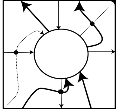
Figure 16: An atomic cobordism which is not $2$-atomic

We say that a checkerboard cobordism is $2$-atomic if $\gamma^{\prime}$ vanishes.

The aim of the present section is to prove the following

Theorem 4.

Assume for a $1$-component framed $4$-graph $K$ we have $L(K)\neq 0$. Then there is no $2$-atomic cobordism spanning the knot $K$ of any genus.

Proof.

Let us revisit the proof of Theorem 3. Assume there is a $2$-atomic cobordism ${\cal D}_{g}\to{\cal D}$ of some genus $g$ spanning the knot $K$. Fix a generic Morse function $f$ on ${\cal D}_{g}$ (the corresponding Morse function on $D_{g}$ will be denoted by the same letter $f$).

Following the lines of the proof of Theorem 3, we see that:

1) at each non-critical level of $f$ we have a free link $L_{c}$ of some number of components, and with each component we associate a natural number coming from a conjugacy class in $G$.

2) these numbers behave nicely under Morse bifurcations, i.e., a birth/death of a circle corresponds to an addition/removal of an occurency of $0$;

3) for a saddle point the three numbers $k,l,m$ corresponding to the adjacent edges satisfy $\pm k\pm l\pm m=0$.

Note that every saddle point merges two circles into one or splits one circle into two circles (the Moebius bifurcation is impossible because ${\cal D}_{g}$ is orientable).

Recall that each of these numbers $k$, $l$, $m$ at this point is defined only up to sign (equivalently, we have an absolute value of these three numbers), and this is not sufficient to prove the theorem in the case of cobordism of arbitrary genus.

Now, let us be more specific and study these numbers on edges in more detail. Let $t$ be a non-critical level of $f$, and let $K_{1},\dots,K_{n}$ be the free knots composing the corresponding free link $K_{t}$. For each of these knots $K_{j}$ we have defined the integer number by taking an initial point of $K_{j}$. This number $2l$ comes from an element of $G$ of the form $x=(bb^{\prime})^{l}$, and we see that a conjugation of $x$ by any of $a,b,b^{\prime}$ takes $x$ to $(b^{\prime}b)^{l}=x^{-1}$. So, a conjugation by a word of even length does not change the number $2l$, whence the conjugation by a word of an odd length takes it to $-2l$.

Let us take a checkerboard colouring of ${\cal D}_{g}$ with respect to the cell decomposition generated by double lines.

Whenever we take an initial point of any section, this initial point does not belong to any double line, so, it has some colour, black or white. We see that a conjugation by a word of even length does not change the colour of the initial point.

This means for every component $K_{j}$, the numbers $l_{b}(K_{j})$ and $l_{w}(K_{j})$ are well defined and $l_{b}(K_{j})=-l_{w}(K_{j})$, where subsripts $b$ and $w$ correspond to the colour choice of the initial point on the circle.

Fix the colour black once forever. Then every edge of the Reeb graph acquires an integer number $l_{b}$, and for every level when we merge/split circles, the sum of these $l_{b}$’s does not change.

So, the sum $l_{b}$ remains invariant for every non-critical level of the Morse function. Since it is non-zero at $t=0$, it will remain non-zero for every $t$.

This completes the proof of theorem 4.

∎

8 Further Directions and Unsolved Problems

8.1 2-knots in 4-space and 4-manifolds

The parity we have defined for double lines for the case of a disc (see section 5) (or a surface with boundary) can be defined just in the same way for a generic map from a $2$-surface to a $4$-manifold.

According to [5, 1], lots of invariants of virtual knots can be refined by using parity. Probably, invariants of $2$-knots in $4$-spaces (say, the quandle) can be refined in the same way by using parity of double lines for $2$-surfaces.

8.2 Gaussian parity and other parities

Another question is whether the same invariant $L$ counted by using another parity and justified parity (not Gaussian) can lead to the same result. This question is closely related to the following question:

Are there any other parities for double lines of $2$-surfaces with singularities and which of them can be obtained as extensions from usual parities of framed $4$-graphs?

8.3 Virtual knots and stronger groups

In [10], a generalization of the group $G$ is constructed; one uses iterated parities by applying the map ${\cal F}$ and counting parities of the obtained chord diagram. In a way similar to the described above, one obtains an invariant of free knots valued in a certain more complicated group. Seemingly, this group will give further obstructions for sliceness; moreover, for flat knots and virtual knots, the group information can be enriched by adding some information about crossings (signs, orientations, etc).

Besides, when we deal not merely with free knots, but with some more complicated objects (virtual knots), we may use more complicated groups [9]. Most probably, the non-triviality of elements of these groups may yield sliceness obstruction for virtual knots.

This problem is especially actual because the sliceness in dimension $4$ has different meanings: a piecewise-flat slice knot might not be smoothly slice. So, it would be very interesting to get some smooth sliceness obstructions

References

- [1] D.M.Afanasiev, On strengthening tnvariants of virtual knots by using parity, Mat. Sb., to appear.
- [2] J.S.Carter (1991), Closed Curves that never extend to proper maps of disks, Proc. Amer. Math. Soc., 113, No. 3, pp. 879-888.
- [3] A.Gibson (2009) Homotopy Invariants of Gauss words, Arxiv:Math.GT./0902.0062
- [4] D.P.Ilyutko, V.O.Manturov, Cobordisms of Free Knots and Gauss words, Arxiv:Math.GT/09042862
- [5] V.O.Manturov (2010), Parity in Knot Theory, Mat. Sb., 2010, 201, 5, pp. 65 110
- [6] V.O.Manturov, On Free Knots, ArXiv:Math.GT/0901.2214 v2
- [7] V.O.Manturov, On Free Knots and Links, ArXiv: Math.GT/0902.0127
- [8] V.O.Manturov, Free Knots and Parity, Arxiv:Math.GT/09125348, v.1., to appear in: Proceedings of the Advanced Summer School on Knot Theory, Trieste, Series of Knots and Everything, World Scientific.
- [9] V.O.Manturov, Free Knots, Groups, and Finite-Type Invariants, ArXiv:Math.GT/1004.4325
- [10] V.O.Manturov, O.V.Manturov, Free Knots and Groups, J. Knot Theory Ramif., to appear.
- [11] Turaev, V.G., Virtual open strings and their cobordisms, preprint, 2004, arXiv: math.GT/ 0311185 v5
- [12] Turaev, V.G., Cobordisms of Words, Arxiv:Math.CO/0511513, v.2.
- [13] Turaev, V.G., Cobordisms of Knots on Surfaces, Arxiv:Math.GT/0703055, v.1.