Atomic and Molecular Systems Driven by Intense Chaotic Light

Abstract

We investigate dynamics of atomic and molecular systems exposed to intense, shaped chaotic fields and a weak femtosecond laser pulse theoretically. As a prototype example, the photoionization of a hydrogen atom is considered in detail. The net photoionization undergoes an optimal enhancement when a broadband chaotic field is added to the weak laser pulse. The enhanced ionization is analyzed using time-resolved wavepacket evolution and the population dynamics of the atomic levels. We elucidate the enhancement produced by spectrally-shaped chaotic fields of two different classes, one with a tunable bandwidth and another with a narrow bandwidth centered at the first atomic transition. Motivated by the large bandwidth provided in the high harmonic generation, we also demonstrate the enhancement effect exploiting chaotic fields synthesized from discrete, phase randomized, odd-order and all-order high harmonics of the driving pulse. These findings are generic and can have applications to other atomic and simple molecular systems.

I INTRODUCTION

The dynamics of atomic and molecular systems exposed to shaped ultrashort, intense light pulses is a subject of great current interest Zewail ; Assion ; RabitPhysTod . The research in this area is motivated by the fact that such light-matter interactions are mostly nonlinear and nonperturbative in nature, thus offering an efficient tool to manipulate atomic and molecular phenomenon on a femtosecond/attosecond time-scale AttoScience . A basic objective of the quantum control is to guide a quantum system from its initial state towards a desired final state selectively with high probability RabitPhysTod . Several quantum control strategies exist in the literature such as, using pump-probe techniques with infrared (IR) and XUV pulses Johnsson ; AttoSpect , implementing closed-loop (iterative) optimization schemes RabitPhysTod , and using open-loop schemes employing tailored light pulses Rabitz-1 .

There is also some work investigating random light fields as a mean to control quantum processes such as bond dissociation kenny , photoionization of neutral atoms kamal_prl or Rydberg atoms NoiseIonRyd , population transfer between energy levels of a system Rabitz-2 and noise autocorrelation spectroscopy milner . This is partly motivated by the fact that under realistic conditions of the laser-matter interaction seemingly random fluctuations are unavoidable. This raises a question about their role on influencing various quantum processes of interest such as photoionization, bond-dissociation, and population transfer between energy levels in a multilevel system etc. Furthermore, it is known that in certain quantum (as well as classical) systems, the presence of noise plays a constructive role via the phenomenon of stochastic resonance (SR) Gamat ; Buchl ; QSR , which can optimize the system response to a weak driving field. SR requires three ingredients: a nonlinear system, a coherent driving, and a noise source Gamat . In principle, all three ingredients are present in atomic and molecular systems interacting with shaped light pulses. Even very intense quasi-random electric-fields can be generated with modern pulse shaping techniques chaoLgt ; MIRshaping ; Weiner which opens up the possibility to employ such chaotic pulses for atomic and molecular systems. Given the vast multitude of pulse shaping possibilities on the one hand side and the fact that, on the other hand, for a large combined effect of coherent driving and noise both must have comparable strength kamal_prl , one needs to identify generic conditions under which chaotic light (with or without a laser pulse) can serve as a control tool and assess how efficient various scenarios are.

In the following, we provide a detailed study of the influence of chaotic light on a single-electron atom interacting with an ultrashort laser pulse. We will demonstrate the role played by chaotic light in optimizing the photoionization process and analyze its properties in the time-domain. After identifying crucial gain-providing frequency-bands under the driving laser pulse, we discuss the efficiency of chaotic light generated using shaped spectral content. In particular, we consider a case when the chaotic light is generated by discrete frequency components analogous to the ones produced in the high harmonic generation process HHG . The features discussed here are generic and can be applied to the problem of molecular dissociation processes.

The article is organized as follows. Section II introduces our model of an atomic system interacting with a femtosecond IR laser pulse and a chaotic light pulse. The method to solve the corresponding time-dependent Schrodinger equation (TDSE) along with useful physical observable is explained. In section III, we show how the chaotic light can produce optimal photoionization enhancement. To characterize the enhancement mechanism, we compute time-resolved wavepacket dynamics and a frequency-resolved gain profile of the driven-atom. We then consider spectrally shaped chaotic lights to optimize the photoionization, in particular, the ones generated by phase randomized even-order and all-order higher harmonic components. Finally, section IV provides a summary of results with our conclusions.

II DESCRIPTION OF THE MODEL

II.1 Atomic and Molecular system exposed to chaotic light and a laser pulse

Let us consider a generic example of an atomic (or molecular) system with one degree of freedom such as the simplest single-electron hydrogen atom. Due to the application of an intense linearly polarized laser field $F(t)$, the electron dynamics is effectively confined in one-dimension along the laser polarization axis Eberly . The Hamiltonian for such a simplified description of the hydrogen atom is written as (atomic units, $\hbar=m=e=1$, are used unless stated otherwise),

$$H(x,t)=H_{0}(x)+xF(t)+xZ(t),$$ (1)

where $x$ is a system coordinate such as the position of the electron and $H_{0}(x)$ is the unperturbed Hamiltonian. The external perturbations, a laser pulse $F(t)$ and a chaotic field $Z(t)$, are dipole-coupled to the system. In the case of an atomic system, the unperturbed Hamiltonian is given by $H_{0}(x)=\frac{\hat{p}^{2}}{2}+V(x)$. The potential $V(x)$ is approximated by a non-singular Coulomb-like form Eberly ,

$$V(x)=-\frac{1}{\sqrt{x^{2}+a^{2}}}.$$ (2)

Such a soft-core potential with parameter $a$ has been routinely employed to study atomic phenomenon in strong laser fields Eberly ; mpi .

Note that a similar one-dimensional model can be used to study the photo-dissociation of diatomic molecules. The potential in that case is the Morse potential. Such model has been used to study for example the molecular dissociation by white shot noise kenny , and using a combination of a white noise with a mid-IR laser pulse kamal . The results on the role of chaotic light on the atomic system can be translated, at least qualitatively, to the case of dissociation dynamics of the diatomic molecules.

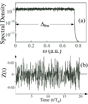
Figure 1: The principle of chaotic light generation. (a) The power spectral density (PSD) of the chaotic light defining its bandwidth $\Delta_{\mathrm{bw}}$. (b) A typical realization of the chaotic electric field $Z(t)$ of bandwidth $0.75$, $N=1024$.

The laser field in Eq. 1 is a nonresonant mid-infrared (MIR) femtosecond pulse described as,

$$\mbox{$F(t)=f(t)F_{0}\sin(\omega_{0}t+\delta)$}.$$ (3)

Here $F_{0}$ defines the peak amplitude of the pulse, $\omega_{0}$ denotes the angular frequency, and $\delta$ is the carrier-to-envelop phase. We choose a smooth pulse envelop $f(t)=\sin^{2}(\pi t/T_{p}))$ where $T_{p}$ is the pulse duration.

The chaotic field term $Z(t)$ consists a normalized sum of $N$ closely spaced oscillators defined as kamal_pra ,

$$Z(t)=\sqrt{\frac{2}{N}}\sum_{n=1}^{N}g(t)F_{\mathrm{rms}}\sin(\omega_{n}t+\phi_{n}),$$ (4)

where $\omega_{n}$, $\phi_{n}$ denotes the angular frequency, phase of $n^{th}$ mode, and $F_{\mathrm{rms}}$ is the root-mean-square amplitude of $Z(t)$. The chaotic light envelop $g(t)$ is chosen such that $g(t)=1$ for $0\leq t\leq T_{p}$ and zero elsewhere. The spacing between two modes $\delta\omega=\omega_{n+1}-\omega_{n}$ is kept very small, so as to have a quasi continuous frequency spectrum [see Fig. 1(a)]. One can define a characteristic bandwidth (BW) of the chaotic light as, $\Delta_{\mathrm{bw}}=N\delta\omega$. Note that here we consider these frequency modes to oscillate independently of each other with their phases $\phi_{n}$ assuming random values relative to each other. In this particular case of phase-randomized coherent modes, the averaged field $Z(t)$ at any point will be noise-like as shown in Fig. 1(b), hence the name chaotic field. Various realizations of the chaotic light are generated by generating different sets of $\phi_{n}$ with uniform probability distribution between 0 to $2\pi$. Note that $Z(t)$ becomes a white noise term in the limit $\Delta_{\mathrm{bw}}\to\infty$ and $\delta\omega\to 0$.

II.2 Quantum dynamics and physical observable

We solve the time-dependent stochastic Schrödinger equation,

$$i\;\frac{\partial\Psi(x,t)}{\partial t}=H(x,t)\;\Psi(x,t),$$ (5)

driven by a chaotic light field and a laser pulse. Due to the presence of the chaotic field term in the Hamiltonian as described above, the quantum evolution is different for each realization of $Z(t)$. This requires to average the final observable of interest over a large number of realizations of $Z(t)$. For a given realization, the numerical solution of the Schrödinger equation amounts to propagating the initial wave function $|\Psi_{0}\rangle$ by computing the infinitesimal short-time stochastic propagator, using a standard split-operator fast Fourier algorithm SOper .

Note that the initial state $|\Psi_{0}\rangle$ is always chosen to be the ground state of the system with an energy of $I_{b}=-0.5$ a.u.. This is obtained by the imaginary-time relaxation method for $a^{2}=2$ Eberly . To avoid parasitic reflections of the wavefunction from the grid boundary, we employ an absorbing boundary SOper .

The main observable of interest for us is the total ionization probability defined as,

$$P=2\int_{0}^{\infty}J_{R}(x_{R},t)dt.$$ (6)

Here $J_{R}(x_{R},t)=Re[\Psi^{\ast}\>\hat{p}\>\Psi]_{x_{R}}$ is the ionization flux QMbook leaking in the continuum where $x_{R}$ is a point near the absorbing boundary. In the following sections, we shall show how the combination of a chaotic field and the laser pulse can enhance photoionization.

III RESULTS AND DISCUSSIONS

III.1 Optimal enhancement of photoionization by chaotic fields

III.1.1 A laser pulse induced femtosecond photoionization

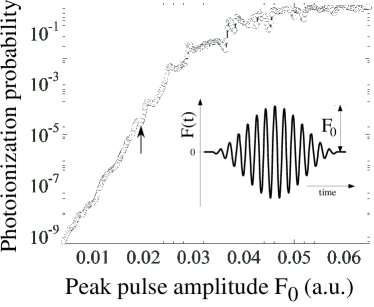
Figure 2: The ionization probability versus the laser peak amplitude $F_{0}$. Inset: schematic of the laser pulse. A vertical arrow on the curve corresponds to a weak laser pulse amplitude, $F_{0}=0.02$.

We shall first consider the atomic photoionization due to a short but strong laser pulse only. As one varies the peak amplitude $F_{0}$ of the mid-IR laser pulse ($\omega=0.057$), the ionization probability first increases nonlinearly, and then saturates to the maximum value of unity, for $F_{0}>0.05$. This behavior of $P_{l}(F_{0})$ is a characteristic signature common to many atomic (or molecular) systems exposed to intense laser pulses mpi .

The laser pulse produces (nonlinear) ionization of the atom which is most easily understood with the picture of tunneling ionization. Ionization flux is produced close to times $t_{k}=[(k+\frac{1}{2})\pi-\delta]/\omega_{0}$ when the effective potential $U(x,t)=V(x)+xF(t)$, is maximally bent down by the dipole-coupled laser field. One can therefore conclude that the photoionization dynamics is highly nonlinear, and in particular it exhibits a form of “threshold” which is defined by the condition for over barrier ionization, $I_{b}=\mathrm{max}_{x}U(x,t_{k})$. From Fig. 2 we identify a “weak” amplitude laser pulse around $F_{0}=0.02$ (see arrows in Fig. 2) such that it produces almost negligible ionization probability. In the following, we shall study the effect of adding a chaotic field on the photoionization process.

III.1.2 Enhancement by addition of the chaotic light

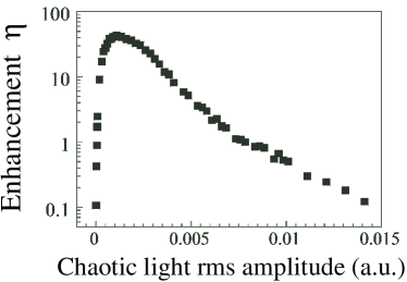
Figure 3: The factor of enhancement $\eta$ plotted versus the rms amplitude of the chaotic light ($\Delta_{\mathrm{bw}}=0.75$, $N=512$). At the maximum of the curve the ratio $F_{\mathrm{rms}}/F_{0}=0.075$. The curve is averaged over 50 different realizations of the chaotic light.

Here we look into the possibility of efficiently ionizing the atom, when it is subjected to both a weak laser pulse ($F_{0}=0.02$) and chaotic light. In order to characterize the stochastic enhancement in the atomic ionization due to interplay between the chaotic field and the laser pulse, we use the following definition of the enhancement factor as kamal

$$\eta=\frac{P_{l+n}-P_{0}}{P_{0}}$$ (7)

where $P_{l}$ is the ionization probability due to laser pulse alone, $P_{n}$ is IP due to chaotic light alone, and $P_{l+n}$ is the one due to the combined action of both the pulses. One can verify that a zero value of $\eta$ corresponds to the case when either the laser pulse ($P_{l}\gg P_{n}$) or the noise ($P_{l}\ll P_{n}$) dominates. Furthermore, $\eta$ characterizes a truly nonlinear quantum interplay as it also vanishes if we assume a “linear” response as a sum of individual probabilities, $P_{l+n}=P_{l}+P_{n}$.

In Fig. 3, we have plotted the enhancement factor $\eta$ versus the rms amplitude $F_{\mathrm{rms}}$ of a broadband chaotic field ($\Delta_{\mathrm{bw}}=0.75$). Each data point is averaged over 50 different realizations of the chaotic light. As the $F_{\mathrm{rms}}$ increases, $\eta$ exhibits a sharp rise, followed by a maximum at a certain value of the (optimum) noise, and then a gradual fall off for very intense chaotic fields. It is worth mentioning that only a modest noise-to-laser ratio ($F_{\mathrm{rms}}/F_{0}=0.075$) is required to reach the optimum enhancement (here $\eta_{\mathrm{max}}=36$). Note that such a curve has been obtained by white Gaussian noise kamal_prl . We have verified that the location of the optimum enhancement is governed by an empirical condition, where the strengths of the laser pulse and noise are comparable such that $P_{l}\sim P_{n}$.

The enhancement curve versus the chaotic light amplitude bears striking resemblance to the typical SR curve where the system response is plotted versus the noise amplitude. However, the observed effect is not the standard SR effect with the characteristic time-scale matching between coherent and incoherent driving. The underlying gain mechanism here is completely different, as we shall see later. In the sense of the existence of an optimum noise level, one can perhaps call this as a generalized quantum SR for such atomic systems on ultrafast time-scales.

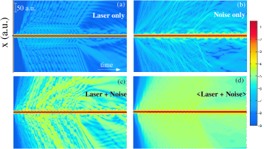
Figure 4: Temporal evolutions of the probability density at the optimal enhancement point of Fig. 3. (a) The case of laser pulse only ($F_{0}=0.02$), (b) Chaotic light only ($F_{\mathrm{rms}}=0.016$), (c) a combination the chaotic light and the laser pulse, (d) same as in (c) but ensemble averaged over 50 different realizations of the chaotic light.

III.2 Analysis of the optimal photoionization enhancement

III.2.1 Time-resolved wavepacket dynamics and level populations

We will now analyze the mechanism of the stochastic enhancement in the time domain. To this end, we compute the wavepacket dynamics and the level populations at the optimum of the enhancement curve. As shown in Fig. 4(a), the weak laser pulse does not yield any significant ionization. Similar is the case when the atom is subjected to the chaotic light alone p[Fig. 4(b)]. The chaotic light induced wavepacket leaking happens at arbitrary instances in time when compared to the one for laser pulse where it takes place regularly near the pulse maxima and minima. When we combine the laser pulse and chaotic light, the ionization flux becomes significantly enhanced, as is clearly visible in Fig. 4(c). Note that the color scale is logarithmic here. Due to the combined action of the laser pulse and noise, significantly higher fraction of the wavepackets is leaked to the continuum. These wavepackets drift away to the continuum and contributes to the enhanced ionization probability. Fig. 4(d) shows the probability density evolution averaged over 50 different realizations of the chaotic light. This ensemble averaging washes out the finer details of the wavepacket dynamics, however, it shows a more homogeneous enhancement of the ionization flux. This shows that one can clearly visualize the photoionization enhancement with wavepacket dynamics.

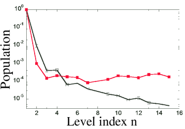
Figure 5: The populations of first fifteen energy levels after the atom has interacted with light pulses corresponding to the optimum of Fig. 3. Filled square: chaotic pulse only $F_{\mathrm{rms}}=0.016$, and open square: The chaotic light with the weak laser pulse, $F_{0}=0.02$.

How does this enhancement manifest itself in the level populations? To answer this, we compute the populations of the first $15$ unperturbed atomic energy levels at the end of the laser pulses. In the case of chaotic light only, the populations of the excited states is small and it decreases as the level index increases (see Fig. 5). However, in the case of simultaneous actions of the laser and chaotic light, the higher excites states populations are significantly enhanced, as one can see in Fig. 5. The population dynamics as well as the wavepacket dynamics clearly show the enhanced excitation (ionization) as a result of the simultaneous action of the laser pulse and noise.

III.2.2 Frequency-resolved gain profile

In order to understand better how the chaotic light enhances ionization in combination with an IR driving, we need to identify the frequency components through which the driven system can absorb energy from the chaotic light since these are not just the atomic lines due to the strong driving. To find out where the driven system absorbs efficiently, we compute a frequency-resolved atomic gain (FRAG) profile $G(\nu)$ using a pump-probe type of setting as described below.

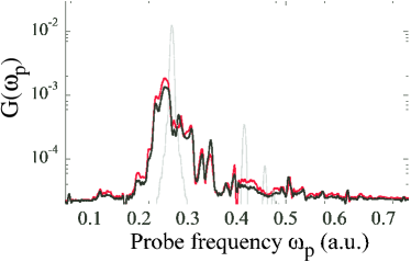
Figure 6: Frequency-resolved gain profile of the atom which is driven by a 10 cycle laser pulse $\omega=0.057$ of amplitude $F_{0}=0.02$. The atomic gain is probed by a synchronized application of a weak probe beam $F_{p}=0.0005$ of tunable frequency $\omega_{p}$. Both the depletion of the ground state population (thick red line) and the net absorption of energy (black) due to the probe are shown. The gain of the bare atom (thin gray line) is also shown for comparison.

We simply replace the chaotic light by a tunable monochromatic probe pulse, $F_{p}(t)=f(t)F_{p}\sin(\omega_{p}t)$. The amplitude $F_{p}$ of the probe is much weaker than the driving laser pulse [$F_{p}/F_{0}=0.025$], such that it does not significantly alter the quasi energy levels, but can drive the transition between them. By preparing the atom in its ground state and measuring the depletion of its population (which indicates the absorbed energy) as a function of the probe frequency $\omega_{p}$, a FRAG profile of the atom is obtained.

Such a gain profile $G(\nu)$ is shown in Fig. 6 for the 10 cycle long laser pulse of amplitude $F_{0}=0.02$. Compared to the pure atomic transitions (thin line) the FRAG shows a complicated structure for the driven atom. The dominated absorption is the slightly red shifted atomic transition frequency between the ground and first excited state, $\omega^{\mathrm{shifted}}_{12}$, but strongly broadened. In fact the broadening is so strong that the driven atom absorbs in the entire frequency regime from $\omega^{\mathrm{shifted}}_{12}\approx 0.25$) to the full binding energy ($\omega_{c}=0.5$). This will have consequences for the enhancement of ionization of the driven atom under chaotic light as we will see below. In particular, we shall employ different variants of chaotic light generated by a variety of spectral shapes to study these consequences in detail.

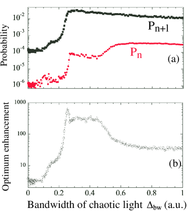
Figure 7: The role of tuning the chaotic light bandwidth $\Delta_{\mathrm{bw}}$ on the optimum enhancement ($F_{0}=0.02$, $F_{\mathrm{rms}}=0.016$). (a) Ionization probabilities versus $\Delta_{\mathrm{bw}}$ for chaotic light only, $P_{n}$, and for a combination of chaotic light and laser pulse, $P_{n+l}$. (b) A corresponding enhancement profile $\eta$ obtained from these probabilities versus $\Delta_{\mathrm{bw}}$.

III.3 Enhancement with spectrally shaped chaotic light

III.3.1 Chaotic light of variable bandwidth

So far we have considered a broadband, quasi-continuous spectrum of the chaotic light. In the following, we shall elucidate the role of different types of spectral shapes of the chaotic light on the ionization enhancement. Firstly, we will vary the bandwidth $\Delta_{\mathrm{bw}}=[0,\omega_{\mathrm{max}}]$ of the chaotic light by lowering the higher cut-off frequency $\omega_{\mathrm{max}}$. The effect of different $\Delta_{\mathrm{bw}}$ on the ionization probability for the chaotic light alone ($P_{n}$) and for its combination with the laser pulse ($P_{l+n}$) is shown in Fig. 7. One can easily understand the curves under the condition that firstly, only one photon of the noise source can be absorbed, yet with any frequency within the bandwidth, and secondly, that the driven system absorbs mainly between the red-shifted transition frequency $\omega^{\mathrm{shifted}}_{12}$ and the cut-off frequency (ionization potential) $\omega_{c}=0.5$ as described above. $P_{n}$ and $P_{l+n}$ exhibit a sharp onset once the bandwidth of the chaotic light covers first transition $\omega_{12}\approx 0.267$. However, a closer inspection reveals that $P_{l+n}$ rises a bit earlier than $P_{n}$ which is due to the fact that under the driving the transition frequency $\omega_{12}$ is red-shifted to $\omega^{\mathrm{shifted}}_{12}\approx 0.25$ (see Fig. 6). Hence, in the optimum enhancement curve (Fig. 7b), there is an overshooting resulting in a sharp peak at $\omega^{\mathrm{shifted}}_{12}$. From $\omega_{12}$ towards higher frequencies, $P_{n+l}$ decreases only slightly. This is also true for $P_{n}$ which, however, “shuts off” with a soft step at the cut-off frequency of $\omega_{c}=0.5$. This is clear from the fact that beyond $\omega_{c}$ the driven atom does not absorb energy (see Fig. 6). The slight decrease of both curves also traces the decreasing availability of the driven atom to absorb light from $\omega_{12}\approx 0.25$ to $\omega=0.5$. For the enhancement this implies overall a plateau between $\omega_{12}$ and $\omega_{c}$ with a sharp onset at $\omega_{12}$ and a soft offset at $\omega_{c}$ to eventually approach the white noise limit for infinite bandwidth. This dependence of enhancement on the bandwidth of the chaotic light suggests that one should use a broad enough bandwidth [covering the plateau of Fig. 7(b)] in order to optimize the enhancement.

III.3.2 Role of quasi-resonant narrow-band chaotic field

The FRAG curve of Fig. 6 shows that the most interesting region in the spectral profile is around the $\omega_{12}$ where one sees a lot of structure. Now we want to consider a special case of system specific narrow band chaotic light centered at the first resonant transition, and widen its bandwidth keeping its central frequency fixed at the $\omega_{12}$. For extremely narrow bandwidth, this essentially becomes a monochromatic light. This example shall also compare the enhancements produced using a single frequency resonant pulse versus the narrowband chaotic light. In Fig. 8 we plot the enhancement curve as a function of rms amplitude of the chaotic light. In the case of very narrow BW, which means that the chaotic light is almost monochromatic, centered at the atomic resonant frequency, one see the enhancement curve. As we increase the BW keeping its central frequency unchanged, the enhancement becomes stronger. This means that although a single frequency laser can provide the photoionization enhancement, the use of broadband chaotic light is preferred if one wants to have a large enhancement factor. With these two cases of narrowband chaotic light and the BW tunable chaotic light, we not only highlight the significance of the FRAG but also show how the chaotic light can be spectrally tuned to a specific system in order to optimize the enhancement profile. The advantage of using a broadband source is that the design becomes independent of both the particular atom and the pulse parameters.

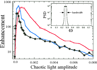
Figure 8: Enhancement induced by a narrow band chaotic light centered at first atomic transition $\omega_{12}=0.267$ as shown in the inset. The enhancement curves for the bandwidths, filled circles: 0.001 (black), open circles: 0.015 (blue), and open squares: 0.2 (red).

III.4 Employing chaotic light generated from discrete harmonics of the driving pulse

It is known that high harmonics (HH) can generate light of extremely broad bandwidth, albeit in the form of discrete frequencies which are integer multiples of the driving laser frequency HHG . The relative phases of these harmonics are either decided in the generation process itself or in the propagation medium. A great deal of efforts has been put into locking their phases to generate attosecond pulses AttoSpect . Here we consider the completely opposite case, where the phases are randomly distributed. This can be realized in principle via their propagation in a suitably chosen medium. For phase randomized HH the net electric field varies almost randomly thus mimicking the chaotic light to some extent. One may wonder if it is possible to use such a discrete set of frequencies to observe the enhancement effect. In the following we consider two different cases where the HH contain, (i) only odd order harmonics of the driving field and, (ii) both even and odd order components. Both these cases are experimentally feasible, the only challenge is to devise an strategy to keep their phases randomized.

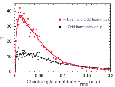
Figure 9: The enhancement curve for a chaotic light with discrete frequency spectrum consisting of $n=1,2,\ldots,6$ higher harmonics of $\omega_{0}=0.057$. Odd-harmonics only: circles, and both even and odd harmonics: squares. Solid lines are average smoothing curves. In both the cases six harmonics ($N=6$) are considered starting from the third one. Each point is averaged over 10 chaotic light realizations.

III.4.1 Use of only odd-order harmonics

Considering the case of phase randomized six odd-order harmonics $\delta\omega=2\omega_{0}$, we assign their phases a random value with a uniform probability density between 0 and $2\pi$. Note that due to equally spaced harmonics the chaotic light time-series would repeat itself after half a laser period. The enhancement curve obtained by averaging over 10 realizations of the HH light is shown in Fig. 9. This suggests an alternative possibility to observe enhancement and underscores the generic nature of the effect, although the maximum enhancement that can be reached in this way is only around $\eta_{\mathrm{max}}=14$. The reason for the relative small enhancement lies again in the FRAG (Fig. 6) since the main absorption at $\omega_{12}^{\mathrm{shifted}}=0.25$ is exactly in the gap of the odd HH used here, namely between $3\omega_{0}=0.171$ and $5\omega_{0}=0.285$. One expects higher enhancement if this gap is filled by all order harmonics.

III.4.2 Use of all-order harmonics

We now consider the possibility of creating nonlinear enhancement of ionization using chaotic light generated from all-order harmonics $\delta\omega=\omega_{0}$. Due to half the frequency spacing compared to odd harmonics only the intrinsic periodicity of the chaotic light is now a full optical cycle. Such an HH spectrum can be experimentally generated by using a two color driving field, by combining the fundamental field by its second harmonic HHG . As one can see in Fig. 9 all-order HH lead to a stronger enhancement with a maximum of around 35 compared to using odd harmonics only, although the total band width covered with the 6 all order harmonics is only half that of odd order harmonics (up to $\omega_{\mathrm{max}}=8\omega_{0}$ compared to $\omega_{\mathrm{max}}=13\omega_{0}$). What really makes the difference is that the all-order HH light has with $4\omega_{0}=0.228$ a frequency component close to the optimum absorption near $\omega_{12}^{\mathrm{shifted}}$.

IV Summary and Conclusion

We have investigated the role of a combined action of a femtosecond laser pulse and chaotic light on a generic quantum phenomenon such as photoionization. Due to the inherent nonlinearity of the strong field ionization process, a dramatic enhancement in ionization yield is observed when a modest amount of optimum chaotic light is added to the weak laser pulse. The mechanism of the enhancement is analyzed using wavepacket evolution as well as level population dynamics.

The key to understanding the enhancement is the frequency-resolved atomic gain profile under the laser pulse which differs substantially from the gain profile of an isolated atom. The ionization enhancement depends on how efficiently the chaotic light supplies strong gain frequencies of the laser-atom system. To elucidate the enhancement we have employed standard broad band chaotic light and beyond it, various shaped chaotic fields such as two different classes of variable bandwidth, one with a variable upper frequency limit and one with a variable bandwidth centered around the main absorption frequency of the laser-atom system. Furthermore, motivated by the extremely broad bandwidth offered by high harmonics, we synthesized chaotic light from phase randomized discrete odd-order harmonics and all-order harmonics. Such chaotic fields also lead to an enhancement profile which suggests an experimental feasibility provided one can randomize the harmonic phases.

We emphasize that the features observed here are of generic nature. Analogous effects can be therefore expected in other atomic and molecular systems, which could be useful for a better understanding of their dynamics as well as for the design of various control strategies using incoherent fields. Dunbar ; Chelk ; Rabitz .

- (1) E. D. Potter et al., Nature 355, 66 (1992).
- (2) A. Assion et al., Science 282, 919 (1998).
- (3) Ian Walmsley and H. Rabitz, Phys. Today, Aug. 43 (2003).
- (4) P. B. Corkum and F. Krausz, Nature Physics 3, 381 (2007).
- (5) P. Johnsson et al., Phys. Rev. Lett 99, 233001 (2007).
- (6) P. H. Bucksbaum, Science 317, 766 (2007).
- (7) A. Pechen and H. Rabitz Phys. Rev. A 73, 062102 (2006).
- (8) A. Kenfack and J. M. Rost, J. Chem. Phys. 123, 204322 (2005).
- (9) Kamal P. Singh and Jan M. Rost Phys. Rev. Lett. 98, 160201 (2007).
- (10) R. Blumel et al., Phys. Rev. Lett. 62, 341 (1989); J. G. Leopold and D. Richards, J. Phys. B 24, L243 (1991); L. Sirko et al., Phys. Rev. Lett. 71, 2895 (1993).
- (11) F. Shuang and H. Rabitz J. Chem. Phys. A 124, 154105 (2006).
- (12) X. G. Xu, S. O. Konorov, J. W. Hepburn, and V. Milner, Nature Physics 4, 125 (2008).
- (13) L. Gammaitoni, P. Hänggi, P. Jung, and F. Marchesoni, Rev. Mod. Phys. 70, 223 (1998).
- (14) T. Wellens, V. Shatokhin, and A. Buchleitner, Rep. Prog. Phys. 67, 45 (2004).
- (15) R. Löfstedt and S. N. Coppersmith, Phys. Rev. Lett 72, 1947 (1994).
- (16) D. Yelin, D. Meshulach, and Y. Silberberg, Opt. Lett. 22, 1793 (1997).
- (17) T. Witte, D. Zeidler, D. Proch, K. L. Kompa, and M. Motzkus Opt. Lett. 27, 1793 (2002).
- (18) A. M. Weiner, Rev. Scien. Instrument 71, 1929 (2000).
- (19) P. Agostini and L. F. DiMauro, Rep. Prog. Phys. 67, 813 (2004).
- (20) M. Protopapas et al., Rep. Prog. Phys. 60, 389 (1997); J. Javanainen, J. H. Eberly and Q. Su, Phys. Rev. A 38, 3430 (1988).
- (21) G. Mainfray and C. Manus, Rep. Prog. Phys. 54, 1333 (1991).
- (22) Kamal P. Singh, A. Kenfack and Jan M. Rost Phys. Rev. A 77, 022707 (2008).
- (23) Kamal P. Singh and Jan M. Rost Phys. Rev. A 76, 063403 (2007).
- (24) J. A. Fleck, J. R. Moris, and M. D. Feit, Appl. Phys. 10, 129 (1976).
- (25) C. Cohen-Tannoudji, B. Diu, and F. Laloë, Quantum Mechanics, Vol. I (Springer-Verlag, Berlin, 1983).
- (26) R. C. Dunbar and T. B. McMahon, Science 279, 194 (1998).
- (27) S. Chelkowski et al., Phys Rev. Lett. 65, 2355 (1990); A. Assion et al., Science 282, 919 (1998).
- (28) H. Rabitz et al., Science 288, 824 (2000).