Tangled Magnetic Fields in Solar Prominences

Abstract

Solar prominences are an important tool for studying the structure and evolution of the coronal magnetic field. Here we consider so-called “hedgerow” prominences, which consist of thin vertical threads. We explore the possibility that such prominences are supported by tangled magnetic fields. A variety of different approaches are used. First, the dynamics of plasma within a tangled field is considered. We find that the contorted shape of the flux tubes significantly reduces the flow velocity compared to the supersonic free fall that would occur in a straight vertical tube. Second, linear force-free models of tangled fields are developed, and the elastic response of such fields to gravitational forces is considered. We demonstrate that the prominence plasma can be supported by the magnetic pressure of a tangled field that pervades not only the observed dense threads but also their local surroundings. Tangled fields with field strengths of about 10 G are able to support prominence threads with observed hydrogen density of the order of $10^{11}$ $\rm cm^{-3}$. Finally, we suggest that the observed vertical threads are the result of Rayleigh-Taylor instability. Simulations of the density distribution within a prominence thread indicate that the peak density is much larger than the average density. We conclude that tangled fields provide a viable mechanism for magnetic support of hedgerow prominences.

1. Introduction

Solar prominences (a.k.a. filaments) are relatively cool structures embedded in the million-degree corona at heights well above the chromosphere (see reviews by Hirayama, 1985; Zirker, 1989; Priest, 1990; Tandberg-Hanssen, 1995; Heinzel, 2007). Above the solar limb, prominences appear as bright structures against the dark background, but when viewed as filaments on the solar disk they can be brighter or darker than their surroundings, depending on the bandpass used to observe them. Magnetic fields are thought to play an important role in supporting the prominence plasma against gravity, and in insulating it from the surrounding hot corona. Most quiescent prominences exhibit intricate filamentary structures that evolve continually due to plasma flows and heating/cooling processes (see examples in Menzel & Wolbach, 1960; Engvold, 1976; Malherbe, 1989; Leroy, 1989; Martin, 1998). In some cases the threads appear to be mostly horizontal, while in other cases they are clearly radially oriented (“hedgerow” prominences). Figure 1 shows several examples of prominences observed in H$\alpha$ at the Big Bear Solar Observatory (BBSO) and the Dutch Open Telescope (DOT). The examples in Figs. 1a and 1b show mainly vertical threads, while the prominence in Fig. 1c shows horizontal threads. Off-limb observations in He II 304 Å indicate that there are higher altitude parts that are optically thin in H$\alpha$ and therefore not visible on the disk (or at least have not been clearly identified in disk observations). Figure 1d shows a prominence above the solar limb as observed in He II 304 Å with the SECCHI/EUVI instrument (Howard et al., 2007) on the STEREO spacecraft. The upper parts of the prominence consist of vertical threads with an intricate fine-scale structure. Movie sequences of quiescent and erupting prominences can be found at the STEREO website.

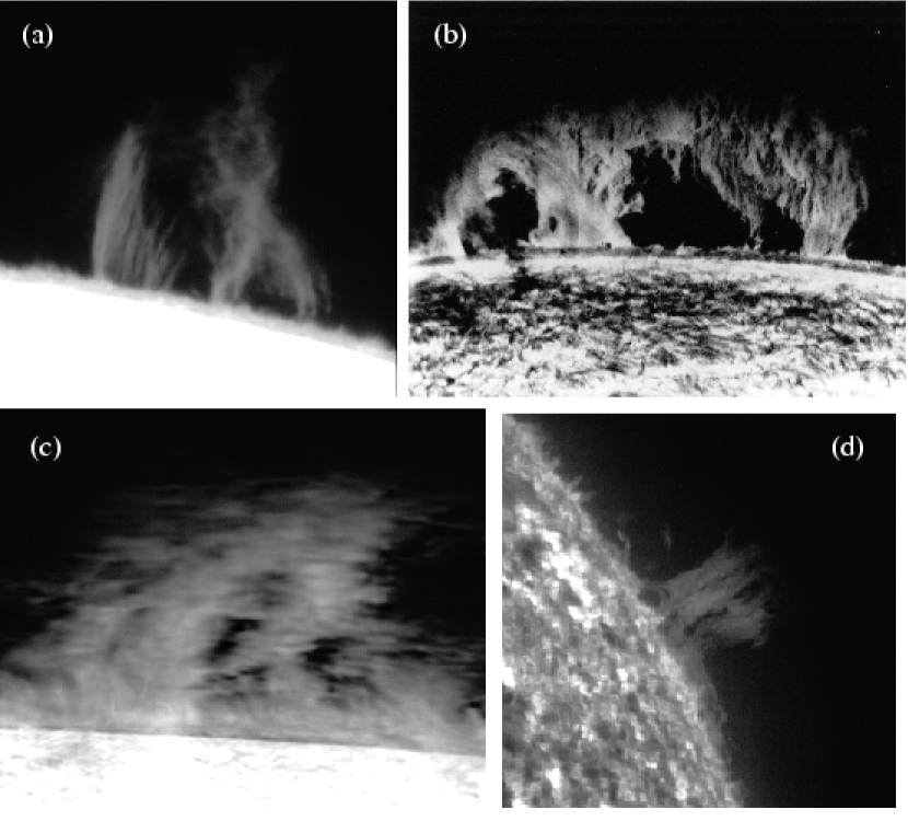
Figure 1.— Quiescent prominences above the solar limb: (a) H$\alpha$ image of prominence observed at Big Bear Solar Observatory (BBSO), November 22, 1995; (b) H$\alpha$, BBSO, 1970; (c) H$\alpha$, Dutch Open Telescope, September 15, 2006; (d) He II 304 Å, STEREO/EUVI, 2008 April 20 at 00:06 UT.

Prominence plasma is highly dynamic, exhibiting horizontal and vertical motions of order 10–70 km s^-1 (Menzel & Wolbach, 1960; Engvold, 1976; Zirker, Engvold & Martin, 1998; Kucera, Tovar & De Pointieu, 2003; Lin, Engvold & Wiik, 2003; Okamoto et al., 2007; Berger et al., 2008; Chae et al., 2008). Recent high-resolution observations of filaments on the solar disk indicate that they consist of a collection of very thin threads with widths of about 200 km, at the limit of resolution of present-day telescopes (Lin, Engvold & Wiik, 2003; Lin et al., 2005a, b; Lin, Martin & Engvold, 2008; Lin et al., 2008). Individual threads have lifetimes of only a few minutes, but the filament as a whole can live for many days. It seems likely that these thin threads are aligned with the local magnetic field. High-resolution images of prominences above the limb have been obtained with the Solar Optical Telescope (SOT) onboard Hinode. For example, Okamoto et al. (2007) observed horizontal threads in a prominence near an active region, and studied the oscillatory motions of these threads. Heinzel et al. (2008) observed a hedgerow prominence consisting of many thin vertical threads, and they used multi-wavelength observations to estimate the amount of absorption and “emissivity blocking” in the prominence and surrounding cavity. Berger et al. (2008) observed another hedgerow prominence and found that the prominence sheet is structured by both bright quasi-vertical threads and dark inclusions. The bright structures are downflow streams with velocity of about 10 km s^-1, and the dark inclusions are highly dynamic upflows with velocity of about 20 km s^-1. The downflow velocities are much less than the free-fall speed, indicating that the plasma is somehow being supported against gravity. Berger et al. (2008) proposed that the dark plumes contain relatively hot plasma that is driven upward by buoyancy. Chae et al. (2008) observed a persistent flow of H$\alpha$ emitting plasma into a prominence from one side, leading to the formation of vertical threads. They suggested that the vertical threads are stacks of plasma supported against gravity by the sagging of initially horizontal magnetic field lines.

Direct measurements of the prominence magnetic field can be obtained using spectro-polarimetry (see reviews by Leroy, 1989; Paletou & Aulanier, 2003; Paletou, 2008; López Ariste & Aulanier, 2007). A comprehensive effort to measure prominence magnetic fields was conducted in the 1970’s and early 1980’s using the facilities at Pic du Midi (France) and Sacramento Peak Observatory (USA). This work showed that (1) the magnetic field in quiescent prominences has a strength of 3–15 G; (2) the field is mostly horizontal and makes an angle of about $40^{\circ}$ with respect to the long axis of the prominence (Leroy, 1989; Bommier & Leroy, 1998; Paletou & Aulanier, 2003); (3) the field strength increases slightly with height, indicating the presence of dipped field lines; (4) most prominences have inverse polarity, i.e., the component of magnetic field perpendicular to the prominence axis has a direction opposite to that of the potential field. These earlier data likely included a variety of quiescent prominences, some with predominantly horizontal threads, others with more vertical threads. In more recent work, Paletou et al. (2001) reported full-Stokes observations of a limb prominence in He I 5876 Å (He $\rm D_{3}$), and derived magnetic field strengths of 30–45 G, somewhat larger than the values reported in earlier studies. Casini et al. (2003) published the first vector-field map of a prominence with a spatial resolution of a few arcseconds. They found that the average magnetic field in this prominence is mostly horizontal with a strength of about 20 G and with the magnetic vector pointing $20^{\circ}$ to $30^{\circ}$ off the prominence axis, consistent with the earlier studies. However, the map also shows clearly organized patches where the magnetic field is significantly stronger than average, up to 80 G (also see Wiehr & Bianda, 2003; López Ariste & Casini, 2002, 2003; López Ariste & Aulanier, 2007; Casini, Bevilacqua & López Ariste, 2005). It is unclear how these patches are related to the fine threads seen at higher spatial resolution. Recently, Merenda et al. (2006) observed He I 10830 Å in a polar crown prominence above the limb, and found evidence for fields of about 30 G that are oriented only $25^{\circ}$ from the vertical direction.

How is the plasma in hedgerow prominences supported against gravity? Many authors have suggested that quiescent prominences are embedded in large-scale flux ropes that lie horizontally above the polarity inversion line (Kuperus & Raadu, 1974; Pneuman, 1983; van Ballegooijen & Martens, 1989; Priest, Hood & Anzer, 1989; Rust & Kumar, 1994; Low & Hundhausen, 1995; Aulanier et al., 1998; Chae et al., 2001; Gibson & Fan, 2006; Dudik et al., 2008). The prominence plasma is thought to be located near the dips of the helical field lines. The magnetic field near the dips may be deformed by the weight of the prominence plasma (Kippenhahn & Schlüter, 1957; Low & Petrie, 2005; Petrie & Low, 2005; Heinzel, Anzer & Gunár, 2005). Others have suggested that the magnetic field in hedgerow prominences is vertical along the observed threads, and that the plasma is supported by MHD waves (Jensen, 1983, 1986; Pecseli & Engvold, 2000). However, relatively high frequencies and wave amplitudes are required, and it is unclear why such waves would not lead to strong heating of the prominence plasma. Dahlburg, Antiochos & Klimchuk (1998) and Antiochos et al. (1999) showed that the prominence plasma can be supported by the pressure of a coronal plasma lower down along an inclined field line; however, this mechanism only works for nearly horizontal field lines (also see Mackay & Galsgaard, 2001; Karpen et al., 2005; Karpen, Antiochos & Klimchuk, 2006; Karpen & Antiochos, 2008). Furthermore, hedgerow prominences are located in coronal cavities where the plasma pressure is very low. Therefore, it seems unlikely that the vertical threads seen in hedgerow prominences can be supported by coronal plasma pressure on nearly vertical field lines.

In this paper we propose that hedgerow prominences are embedded in magnetic fields with a complex “tangled” structure. Such tangled fields have many dips in the field lines where the weight of the prominence plasma can be counteracted by upward magnetic forces. Our purpose is to demonstrate that such tangled fields provide a viable mechanism for prominence support in hedgerow prominences. Casini, Manso Sainz & Low (2009) recently invoked tangled fields in the interpretation of spectropolarimetric observations of an active region filament. While such filaments are quite different from the hedgerow prominences considered here, this work shows that tangled fields have important effects on the measurement of prominence magnetic fields. Such effects will not be considered in this paper.

The paper is organized as follows. In Section 2 we propose that hedgerow prominences are supported by tangled magnetic fields, and we discuss how such fields may be formed. In Section 3 we present a simple model for the dynamics of plasma along the tangled field lines, and we show that weak shock waves naturally occur in such plasmas. In Section 4 we develop a magnetostatic model of tangled fields based on the linear force-free field approximation, and in Section 5 we study the response of such fields to gravitational forces. In Section 6 we simulate the distribution of plasma in a cylindrical prominence thread. In Section 7 we discuss the formation of vertical threads by Rayleigh-Taylor instability. The results of the investigation are summarized and discussed in Section 8.

2. Tangled Fields in Prominences

The spectro-polarimetric observations of prominences described in Section 1 are consistent with the idea that quiescent prominences are embedded in coronal flux ropes that lie horizontally above the polarity inversion line (PIL). Figure 2a shows a vertical cross-section through such a flux rope. The magnetic field also has a component into the image plane, so the field lines are helices, and the plasma is assumed to be located at the dips of these helical windings. A dip is defined as a point where the magnetic field is locally horizontal and curved upward. As indicated in the figure, the magnetic field may be deformed by the weight of the prominence plasma, creating V-shaped dips. The magnetic field near such dips is well described by the Kippenhahn-Schlüter model (Kippenhahn & Schlüter, 1957), and several authors have developed local magnetostatic models of the fine structures observed in quiescent prominences (e.g., Low, 1982; Petrie & Low, 2005; Heinzel, Anzer & Gunár, 2005). However, recent observations of “dark plumes” (Berger et al., 2008) and rotational motions (Chae et al., 2008) within prominences remind us again that prominences have complex internal motions, and it is not clear how such motions can be explained in terms of a single large flux rope. Perhaps the magnetic structure of hedgerow prominences is more complicated than that predicted by the flux rope model (Figure 2a).

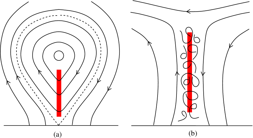
Figure 2.— Magnetic support of solar prominences: (a) by a large-scale coronal flux rope, (b) by a tangled magnetic field in a current sheet.

In this paper we propose an alternative model, which is illustrated in Figure 2b. Following Kuperus & Tandberg-Hanssen (1967), we suggest that hedgerow prominences are formed in current sheets that overlie certain sections of the PIL on the quiet Sun. Unlike those previous authors we suggest that the current sheet extends only to limited height ($\sim 100$ Mm), and may extend only a limited distance along the PIL. Furthermore, we propose that tangled magnetic fields are present within these current sheets. A tangled field is defined as a magnetic structure in which the field lines are woven into an intricate fabric, and individual field lines follow nearly random paths. We suggest that the field is tangled on a spatial scale of 0.1–1 Mm, comparable to the pressure scale height $H_{p}$ of the prominence plasma ($H_{p}\approx 0.2$ Mm). The prominence plasma is assumed to be located at the many dips of the tangled field lines. The tangled field is confined horizontally by the vertical fields on either side of the sheet, and vertically by the weight of the prominence plasma.

A key feature of a tangled field is that the plasma and field are in magnetostatic equilibrium, i.e., the Lorentz force is balanced by the gas pressure gradients and gravity. Therefore, a tangled field is quite different from “turbulent” magnetic fields in which large-amplitude Alfvén waves are present (e.g., the solar wind). In a tangled field the magnetic perturbations do not propagate along the field lines. In this paper we examine the basic properties of tangled fields, and we investigate their ability to support the prominence plasma.

We suggest that the tangled field may be formed as a result of magnetic reconnection, not the twisting or stressing of field lines. Quiescent prominences are located above polarity inversion “lines” that are often more like wide bands of mixed polarity separating regions with dominantly positive and negative polarity. In these mixed-polarity zones, magnetic flux elements move about randomly and opposite polarity elements may cancel each other (e.g., Livi, Wang & Martin, 1985). New magnetic bipoles frequently emerge from below the photosphere. These processes causes the “recycling” of the photospheric flux about once every 2 to 20 hours (Hagenaar, Schrijver & Title, 2003; Hagenaar, DeRosa & Schrijver, 2008), and the coronal flux is recycled even faster (Close et al., 2005). It is likely that the interactions between these flux elements produce a complex, non-potential magnetic field in the low corona. Within this environment magnetic reconnection is likely to occur frequently at many different sites in the corona above the inversion zone. Each reconnection event may produce a bundle of twisted field, and the twisted fields from different events may collect into larger conglomerates to form a tangled field. The tangled field may rise to larger heights (as a result of its natural buoyancy), and may collect into a thick sheet that is sandwiched between smoother fields, as illustrated in Figure 2b. The observed prominence consists of plasma that is trapped within this sheet. New tangled field is continually injected into the sheet from below, producing vertical motions within the sheet. We suggest that the “dark plumes” observed by Berger et al. (2008) may be a manifestation of such vertical motions of the tangled field.

3. Flows Along the Tangled Field

The spatial distribution of plasma within the prominence is determined in part by the dynamics of plasma along the tangled field lines. Figure 3 shows the contorted (but generally downward) path of an individual field line in the tangled field. Note that there are several “dips” where the field line is horizontal and curved upward, and “peaks” where the field is horizontal and curved downward. Tracing the field line upward from a dip, one always reaches a peak where the field line again turns downward. Therefore, the question arises whether the plasma collected in the dips would remain in these dips or be siphoned out of the dips via the peaks of the field lines.

Figure 3.— Flows along a highly distorted field line in the tangled magnetic field of a solar prominence. The field line is indicated by the solid curve, and the black dots indicate “dips” in the field line where cool prominence plasma can collect. The arrows show the direction of subsonic (blue) and supersonic (red) flows. Sonic points are located at peaks in the field lines (black vertical bars), and shock waves occur where supersonic flows slow down before reaching a dip (magenta bars).

To answer this question, we consider a simple model for the motion of the prominence plasma along the magnetic field. For simplicity we assume that the flow takes place in a thin tube surrounding the selected field line (i.e., the divergence of neighboring field lines is neglected), and the cross-sectional area of this tube is taken to be constant. We assume a steady flow is established along the tube. Let $v(s)$ and $\rho(s)$ be the plasma velocity and density as functions of position $s$ along the tube, then conservation of mass requires $\rho v$ = constant. The equation of motion of the plasma is

$$\rho v\frac{dv}{ds}=-\frac{dp}{ds}-\rho g\frac{dz}{ds},$$ (1)

where $p(s)$ is the plasma pressure, $z(s)$ is the height above the photosphere, and $g$ is the acceleration of gravity. The equation of state is written in the form $p=K\rho^{\gamma}$, where $\gamma$ and $K$ are constants (we use $\gamma<5/3$ to describe non-adiabatic processes). Eliminating $p(s)$ and $\rho(s)$ from equation (1), we obtain the following equation for the parallel flow velocity:

$$\left(v-\frac{c^{2}}{v}\right)\frac{dv}{ds}=-g\frac{dz}{ds},$$ (2)

where $c(s)$ is the sound speed ($c^{2}\equiv\gamma p/\rho$). The above equation has a critical point where the flow velocity equals the sound speed ($v=c$). Therefore, a transition from subsonic to supersonic flow can occur only at points where the RHS of this equation vanishes, $dz/ds=0$. These sonic points are located at the peaks of the field lines where matter can be siphoned out of one dip and deposited into another dip at lower height. The resulting flow pattern is indicated in Figure 3. As the supersonic flow approaches the next dip, it must slow down to subsonic speeds, which can only happen in a shock. Therefore, the tube has a series of subsonic and supersonic flows separated by shocks and sonic points. The role of these shocks is to dissipate the gravitational energy that is released by the falling matter.

The position and strength of the shocks can be computed if the height $z(s)$ of the flow tube is known. Neighboring peaks are generally not at the same height. Therefore, each section between neighboring peaks is approximated as a large-amplitude sinusoidal perturbation superposed on a generally downward path:

$$z(s)\approx A\cos\left(2\pi\frac{s}{\Lambda}-\phi_{0}\right)-Cs,$$ (3)

where $s$ is the position along the flow tube, $\Lambda$ is the distance between neighboring peaks (as measured along the flow tube), $A$ is the amplitude of the perturbation in height, $\phi_{0}$ is a phase angle, and $C$ is the background slope. The phase angle is chosen such that the peaks in the flow tube (where $dz/ds=0$) are located at $s=0$ and $s=\Lambda$, then the slope is given by

$$C=2\pi\frac{A}{\Lambda}\sin\phi_{0}.$$ (4)

The sonic points will then be located at $s=0$ and $s=\Lambda$.

Figure 4.— Model for plasma flow along a single field line in a tangled field. (a) The solid curve shows the height $z(s)$ as function of position $s$ along the field line [in units of the distance $\Lambda$ between neighboring peaks, see equation (3)]. The dashed curve shows the overall downward trend of the flow tube. (b) The solid curve shows the parallel flow velocity $v(s)$ (in units of $c_{0}$) for $\gamma=1.5$ and $H_{p,0}=0.15\Lambda$. The dashed curves show the subsonic and supersonic solutions of equation (6). The sonic points are located at the peaks in the field line ($s=0$ and $s=\Lambda$), and the shock is located at $s=0.325\Lambda$. (c) Similar plot for the sound speed $c(s)$ (in units of $c_{0}$). (d) The solid curve shows the plasma density $\rho(s)$ along the tube (in arbitrary units). The hydrostatic equilibrium density is shown by the dashed curve.

Figure 4a shows the height $z(s)$ for $A=0.15\Lambda$ and $\phi_{0}=0.2$ rad, so that $C=0.187$. Let $p_{0}$, $\rho_{0}$ and $c_{0}$ be the pressure, density and sound speed at the sonic points, then $K=\gamma^{-1}c_{0}^{2}\rho_{0}^{1-\gamma}$, and the sound speed can be written as

$$c(s)=c_{0}[\rho(s)/\rho_{0}]^{(\gamma-1)/2}=c_{0}[v(s)/c_{0}]^{-(\gamma-1)/2}.$$ (5)

Inserting this expression into equation (2), we obtain

$$\left(u-u^{-\gamma}\right)\frac{du}{ds}=-\frac{1}{\gamma H_{p,0}}\frac{dz}{ds},$$ (6)

where $u(s)\equiv v(s)/c_{0}$, and $H_{p,0}\equiv p_{0}/(\rho_{0}g)$ is the pressure scale height at the sonic points. Equation (6) can be integrated as follows:

$$\text@frac{1}{2}[u^{2}(s)-1]+\frac{1}{\gamma-1}\left[u^{1-\gamma}(s)-1\right]=-\frac{z(s)-z(s_{0})}{\gamma H_{p,0}},$$ (7)

where $s_{0}$ is the position of a sonic point. Equation (7) can be solved for $u(s)$ by Newton-Raphson iteration. When $\gamma=1$, there is an analytic solution for $u(s)$ in terms of the Lambert $W$ function (see Cranmer, 2004); in the present paper we assume $\gamma=1.5$. The supersonic solution $v_{1}(s)$ is computed with $s_{0}=0$, and the subsonic solution $v_{2}(s)$ is computed with $s_{0}=\Lambda$. The dashed curves in Figure 4b show $v_{1}(s)$ and $v_{2}(s)$, and Figure 4c shows the corresponding sound speeds $c_{1}(s)$ and $c_{2}(s)$. Here we assumed a scale height $H_{p,0}=0.15\Lambda$, equal to the amplitude of the field-line distortions. The Mach number of the flow is given by

$$M(s)=v(s)/c(s)=[u(s)]^{(\gamma+1)/2}.$$ (8)

The shock is located at the point $s_{sh}$ where the Mach number $M_{1}$ before the shock and the Mach number $M_{2}$ after the shock satisfy the following relationship:

$$M_{2}^{2}=\frac{2+(\gamma-1)M_{1}^{2}}{2\gamma M_{1}^{2}-(\gamma-1)},$$ (9)

which follows from the Rankine-Hugionot conditions for parallel shocks (Landau & Lifshitz, 1959). Therefore, the actual flow velocity $v(s)$ between the two sonic points is given by the full curve in Figure 4b, and the sound speed $c(s)$ is given by the full curve in Figure 4c.

The plasma density $\rho(s)$ along the flow tube is determined by mass conservation ($\rho v$ = constant), and is plotted in Figure 4d. Note that there is a strong peak in the density at the dip in the field line, $s_{dip}\approx 0.56\Lambda$. The dashed curve in Figure 4d shows the density profile that would exist if the plasma were in hydrostatic equilibrium (HE):

$$\rho_{HE}(s)=\rho_{dip}\exp\left[-\frac{z(s)-z(s_{dip})}{H_{p}}\right],$$ (10)

where $\rho_{dip}$ and $H_{p}$ are the density and pressure scale height at the dip, $H_{p}=0.254\Lambda$. The deviations from hydrostatic equilibrium are significant only in those regions where the flow velocity is comparable to the sound speed. We define an average flow velocity $\bar{v}$ by

$$\bar{v}\equiv\frac{\int_{0}^{\Lambda}\rho(s)v(s)ds}{\int_{0}^{\Lambda}\rho(s)ds}=\frac{\Lambda}{\int_{0}^{\Lambda}v^{-1}(s)ds}.$$ (11)

For the case shown in Figure 4 we find $\bar{v}=0.6c_{0}$, so the average flow speed is less than the sound speed. Therefore, the contorted shape of the flow tube significantly reduces the flow velocity compared to the supersonic free fall that would occur in a straight vertical tube.

The cooler parts of the prominence are thought to have a temperature $T\sim 10^{4}$ K. Assuming a hydrogen ionization fraction of 10%, a helium abundance of 10 % and $\gamma=1.5$, the sound speed $c_{0}\approx 10$ km s^-1, and we predict an average flow velocity $\bar{v}\approx 0.6c_{0}\approx 6$ km s^-1. The vertical component of this velocity is $\bar{v}_{z}\approx-C\bar{v}\approx-1.1$ km s^-1, less than the observed vertical velocities in prominence threads (5–10 km s^-1). Note that the predicted velocity is relative to the pattern of the tangled field, therefore, if the tangled field expands in the vertical direction it will push the prominence plasma upward. We speculate that the observed upward motions in hedgerow prominences (e.g., Berger et al., 2008) are due to such large-scale changes in the tangled field.

4. Linear Force-Free Field Models

In this section simple models for tangled fields are developed. A volume $V$ in the corona is considered, and the plasma inside this volume is assumed to be in magnetostatic equilibrium, $-\nabla p+\rho{\bf g}+{\bf F}=0$, where $p$ is the plasma pressure, $\rho$ is the density, ${\bf g}$ is the acceleration of gravity, and ${\bf F}$ is the Lorentz force. All quantities are functions of position ${\bf r}$ within the volume. The Lorentz force is given by

$${\bf F}\equiv\frac{1}{c}{\bf j}\times{\bf B}=\frac{1}{4\pi}(\nabla\times{\bf B})\times{\bf B},$$ (12)

where ${\bf j}$ is the electric current density and ${\bf B}$ is the magnetic field. Using tensor notation, equation (12) can also be written as $F_{i}=\partial T_{ij}/\partial x_{j}$, where $T_{ij}$ is the magnetic stress tensor, a special case of Maxwell’s stress tensor (Jackson, 1999):

$$T_{ij}\equiv-\frac{B^{2}}{8\pi}\delta_{ij}+\frac{B_{i}B_{j}}{4\pi}.$$ (13)

The first term describes magnetic pressure, and the second term describes magnetic tension. In a tangled field both pressure and tension forces are important.

If gravity and plasma pressure gradients are neglected, then ${\bf F}\approx 0$, so the magnetic field ${\bf B}({\bf r})$ must satisfy the force-free condition:

$$\nabla\times{\bf B}=\alpha{\bf B},$$ (14)

where $\alpha({\bf r})$ may in general be a function of position. In the special case that $\alpha$ is constant throughout the volume, equation (14) becomes a linear equation for ${\bf B}({\bf r})$, and the solutions are called linear force free fields (LFFF). Woltjer (1958) has shown that in a closed magnetic system with a prescribed magnetic helicity ($H\equiv\int{\bf A}\cdot{\bf B}dV$, where ${\bf A}$ is the vector potential) the lowest-energy state is a LFFF. Therefore, in this paper only LFFFs are considered, and $\alpha$ is treated as a free parameter. We find that LFFFs can be tangled. The typical length scale of the tangled field is given by the inverse of the $\alpha$ parameter, $\ell\equiv|\alpha|^{-1}$. In the following we first consider the case that $\ell$ is small compared to the domain size $L$ in any direction, and then consider the boundary effects. Section 4.3 describes tangled fields in a cylindrical domain.

4.1. Tangled Field in a Large Volume

In the absense of boundary conditions, the solution of equation (14) can be written as a superposition of planar modes:

$${\bf B}({\bf r})=\sum_{n=1}^{N}B_{n}\left[\hat{\bf e}_{1,n}\cos({\bf k}_{n}\cdot{\bf r}+\beta_{n})-\hat{\bf e}_{2,n}\sin({\bf k}_{n}\cdot{\bf r}+\beta_{n})\right],$$ (15)

where $N$ is the number of modes, ${\bf k}_{n}\equiv\alpha\hat{\bf e}_{3,n}$ is the wave vector ($n=1,\cdots,N$), $B_{n}$ is the mode amplitude, $\beta_{n}$ is a phase angle, and $[\hat{\bf e}_{1,n},\hat{\bf e}_{2,n},\hat{\bf e}_{3,n}]$ are unit vectors that are mutually orthogonal and form a right-handed basis system:

$$\hat{\bf e}_{1,n} = \cos\theta_{n}(\cos\phi_{n}~{}\hat{\bf y}+\sin\phi_{n}~{}\hat{\bf z})-\sin\theta_{n}~{}\hat{\bf x},$$ (16)

$$\hat{\bf e}_{2,n} = -\sin\phi_{n}~{}\hat{\bf y}+\cos\phi_{n}~{}\hat{\bf z},$$ (17)

$$\hat{\bf e}_{3,n} = \sin\theta_{n}(\cos\phi_{n}~{}\hat{\bf y}+\sin\phi_{n}~{}\hat{\bf z})+\cos\theta_{n}~{}\hat{\bf x}.$$ (18)

Here $\theta_{n}$ and $\phi_{n}$ are the direction angles of the wave vector relative to the Cartesian reference frame.

Figure 5 shows an example of a field with $N=100$ modes, an isotropic distribution of direction angles $(\theta_{n},\phi_{n})$, and randomly selected phase angles $\beta_{n}$. The starting points of the field lines are randomly selected from the central part of the box, and the field lines are traced until they reach the box walls. Note that individual field lines follow random paths, and that different field lines are tangled together.

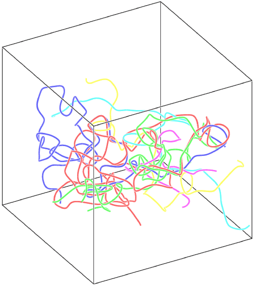
Figure 5.— Tangled field obtained by superposition of 100 randomly selected modes of the linear force-free field in a large volume.

Now consider an ensemble ${\cal E}_{\beta,N}$ of fields with different (randomly distributed) phase angles $\beta_{n}$, but with a fixed number of modes $N$, and with fixed mode amplitudes $B_{n}$ and direction angles $(\theta_{n},\phi_{n})$. The phase angles are assumed to be uniformly distributed in the range $[0,2\pi]$, and angles from different modes $n$ and $n^{\prime}$ are assumed to be uncorrelated. Then the ensemble average of the magnetic field vanishes,

$$<{\bf B}>_{\beta}=0,$$ (19)

where $<\cdots>_{\beta}$ denote the average over phase angles $\beta_{n}$. Also, the average of the tensor ${\bf B}{\bf B}$ is given by

$$<{\bf B}{\bf B}>_{\beta}\,\,=\,\text@frac{1}{2}\sum_{n=1}^{N}B_{n}^{2}\left(\hat{\bf e}_{1,n}\hat{\bf e}_{1,n}+\hat{\bf e}_{2,n}\hat{\bf e}_{2,n}\right)$$

$$\,\,\,\,\,=\,\text@frac{1}{2}\sum_{n=1}^{N}B_{n}^{2}\left({\bf I}-\hat{\bf e}_{3,n}\hat{\bf e}_{3,n}\right),$$ (20)

where ${\bf I}$ is the unit tensor (${\bf I}=\hat{\bf x}\hat{\bf x}+\hat{\bf y}\hat{\bf y}+\hat{\bf z}\hat{\bf z}$). Expression (20) is independent of position ${\bf r}$, so the magnetic field is statistically homogeneous, but is not necessarily isotropic.

We study the statistical properties of field lines in models with different values of the mode number $N$. For each $N$ we construct a series of models ($m=1,\cdots,M$) with different phase angles, but with constant values of the mode amplitudes $B_{n}$ and direction angles $(\theta_{n},\phi_{n})$. The mode amplitudes are taken to be the same for all modes ($B_{n}=1$). For each realization $m$ of the phase angles $\beta_{n}$ we trace out the field line that starts at the origin ($x=y=z=0$), and we measure the square of the radial distance $r_{m}^{2}(s)$ as function of position $s$ along the field line:

$$r_{m}^{2}(s)=x_{m}^{2}(s)+y_{m}^{2}(s)+z_{m}^{2}(s).$$ (21)

We then average this quantity over $M=100$ realizations of the phase angles to obtain the mean square distance $\overline{r^{2}}(s)$. For $N=3$ both mutually orthogonal directions $(\theta_{n},\phi_{n})$ and randomly chosen directions are considered. In both cases we find that the field lines follow long helical paths, and $\overline{r^{2}}(s)$ increases quadratically with $s$. Therefore, for $N=3$ the field lines do not behave randomly. For $N\geq 4$ only randomly chosen directions are considered. For $N=4$ some of the field lines are long helices, while others have more random paths, and for $N=5$ all field lines seem random, however, in both cases $\overline{r^{2}}(s)$ is not well fit by a power law. True random walk behavior of the field lines, as indicated by a linear dependence of $\overline{r^{2}}$ on distance $s$, is found only when the number of modes is increased to $N\geq 10$. In the limit of large $N$, $\overline{r^{2}}(s)\approx 10s/|\alpha|$.

We now consider a larger ensemble ${\cal E}_{N}$ in which not only the phase angles $\beta_{n}$ but also the mode amplitudes $B_{n}$ and direction angles $(\theta_{n},\phi_{n})$ are allowed to vary. From now on $<\cdots>$ will denote an average over this larger ensemble. The direction angles are assumed to have an isotropic distribution, i.e., the angle $\phi_{n}$ is uniformly distributed in the range $[0,2\pi]$, and $\cos\theta_{n}$ is uniform in the range $[-1,+1]$, so that $<\cos^{2}\theta_{n}>=\text@frac{1}{3}$. Furthermore, the mode amplitudes $B_{n}$ are assumed to be uncorrelated with the direction angles, and $<B_{n}^{2}>=B_{0}^{2}/N$, where $B_{0}$ is a constant. Then $<{\bf B}>=0$, so the mean magnetic field vanishes. Further averaging of equation (20) shows that $<{\bf B}{\bf B}>$ is an isotropic tensor:

$$<{\bf B}{\bf B}>=\text@frac{1}{2}\sum_{n=1}^{N}<B_{n}^{2}>\left({\bf I}-<\hat{\bf e}_{3,n}\hat{\bf e}_{3,n}>\right)=\text@frac{1}{3}B_{0}^{2}{\bf I}.$$ (22)

It follows that $<B^{2}>=B_{0}^{2}$, so $B_{0}$ equals the r.m.s. value of the total field strength. The ensemble average of the magnetic stress tensor, equation (13), is given by

$$<T_{ij}>=-\frac{B_{0}^{2}}{24\pi}\delta_{ij},$$ (23)

which is also isotropic. Note that the diagonal components of $<T_{ij}>$ are negative, so the effects of magnetic pressure dominate over the effects of magnetic tension. Therefore, the isotropic tangled field has a positive magnetic pressure, $p_{t}=B_{0}^{2}/(24\pi)$. The average energy density is $E_{t}=B_{0}^{2}/(8\pi)$. The relationship $E_{t}=3p_{t}$ is similar to that for a relativistic gas (e.g., Weinberg, 1972).

4.2. Boundary Effects

The tangled field must be confined within a certain volume (e.g., a current sheet, see Figure 2b), and the confinement must be effective for a period much longer than the Alfven travel time across the volume. What are the conditions for such confinement? To answer this question we must consider the boundary region between a tangled field and a smooth field. The tangled field is assumed to be characterized by a high value of $|\alpha|$, and the smooth field presumably has a much lower value of $|\alpha|$. To last a long time, the magnetic field near the boundary must be approximately in equilibrium (non-linear force-free field). The force-free condition (14) implies that $\alpha$ is constant along field lines, so there cannot be many field lines that pass from the smooth region to the tangled region. Therefore, one important condition for the survival of the tangled field is that the two regions are nearly disconnected from each other magnetically. Another requirement is that the two regions are approximately in pressure balance.

To show that these conditions can be satisfied, we now consider a simple model for the boundary region. The interface between the tangled and smooth fields is approximated by a plane surface, here taken to be the plane $x=0$ in Cartesian coordinates. The above-mentioned condition on the lack of connectivity between the smooth and the tangled fields requires $B_{x}(0,y,z)=0$ at $x=0$. The tangled field in $x\geq 0$ is assumed to be a LFFF with a specified value of $\alpha$. The solution of the LFFF equation is again written as a superposition of planar modes. However, in the present case the modes are grouped into pairs with closely related wave vectors ${\bf k}_{n}$ and ${\bf k}_{n}^{\prime}$, and with the same amplitude $B_{n}$ and phase $\beta_{n}$:

$${\bf B}({\bf r}) = \sum_{n=1}^{N/2}B_{n}\left[\hat{\bf e}_{1,n}\cos({\bf k}_{n}\cdot{\bf r}+\beta_{n})-\hat{\bf e}_{2,n}\sin({\bf k}_{n}\cdot{\bf r}+\beta_{n})\right.$$ (24)

$$\left.\cdots\,\,-\hat{\bf e}_{1,n}^{\prime}\cos({\bf k}_{n}^{\prime}\cdot{\bf r}+\beta_{n})+\hat{\bf e}_{2,n}\sin({\bf k}_{n}^{\prime}\cdot{\bf r}+\beta_{n})\right].$$

Here $N$ is the total number of modes, $\hat{\bf e}_{1,n}$ and $\hat{\bf e}_{2,n}$ are defined in equations (16) and (17), ${\bf k}_{n}^{\prime}\equiv\alpha\hat{\bf e}_{3,n}^{\prime}$ is the modified wave vector, and the unit vectors $\hat{\bf e}_{1,n}^{\prime}$ and $\hat{\bf e}_{3,n}^{\prime}$ are defined by

$$\hat{\bf e}_{1,n}^{\prime} = -\cos\theta_{n}(\cos\phi_{n}~{}\hat{\bf y}+\sin\phi_{n}~{}\hat{\bf z})-\sin\theta_{n}~{}\hat{\bf x},$$ (25)

$$\hat{\bf e}_{3,n}^{\prime} = ~{}~{}\sin\theta_{n}(\cos\phi_{n}~{}\hat{\bf y}+\sin\phi_{n}~{}\hat{\bf z})-\cos\theta_{n}~{}\hat{\bf x}.$$ (26)

Note that $\hat{\bf e}_{3,n}^{\prime}$ differs from $\hat{\bf e}_{3,n}$ only in the sign of the $x$-component, whereas $\hat{\bf e}_{1,n}^{\prime}$ has the sign of the $y$- and $z$-components reversed. Therefore, the unit vectors $[\hat{\bf e}_{1,n}^{\prime},\hat{\bf e}_{2,n},\hat{\bf e}_{3,n}^{\prime}]$ again form a right-handed basis system. The magnetic field at the boundary ($x=0)$ is given by

$${\bf B}(0,y,z)=2\sum_{n=1}^{N/2}B_{n}\cos\theta_{n}(\cos\phi_{n}~{}\hat{\bf y}+\sin\phi_{n}~{}\hat{\bf z})$$

$$\times\,\,\cos\left[\alpha\sin\theta_{n}(y\cos\phi_{n}+z\sin\phi_{n})+\beta_{n}\right],$$ (27)

which satisfies $B_{x}(0,y,z)=0$. Therefore, it is possible to construct a tangled field that is disconnected from its surroundings.

We now consider the statistical average of the tensor ${\bf B}{\bf B}$ at $x=0$. Averaging over phase angles $\beta_{n}$, we obtain

$$<{\bf B}{\bf B}>_{\beta}\,=2\sum_{n=1}^{N/2}B_{n}^{2}\cos^{2}\theta_{n}(\cos\phi_{n}~{}\hat{\bf y}+\sin\phi_{n}~{}\hat{\bf z})$$

$$\times\,\,(\cos\phi_{n}~{}\hat{\bf y}+\sin\phi_{n}~{}\hat{\bf z})~{}~{}~{}\mbox{at}~{}x=0,$$ (28)

and further averaging over mode amplitudes and direction angles yields

$$<{\bf B}{\bf B}>=\frac{1}{6}B_{0}^{2}(\hat{\bf y}\hat{\bf y}+\hat{\bf z}\hat{\bf z})~{}~{}~{}\mbox{at}~{}x=0.$$ (29)

Here we assume an isotropic distribution of direction angles, and we use $<B_{n}^{2}>=B_{0}^{2}/N$, where $B_{0}$ is the r.m.s. field strength in the interior of the tangled field (see Section 4.1). Note that at the boundary $<B^{2}(0,y,z)>=B_{0}^{2}/3$, while in the interior $<B^{2}>=B_{0}^{2}$, so the r.m.s. field strength at the boundary is reduced by a factor $1/\sqrt{3}$ compared to that in the interior. The magnetic pressure at $x=0$ is given by

$$\frac{B_{ext}^{2}}{8\pi}\approx\frac{<B^{2}(0,y,z)>}{8\pi}=\frac{B_{0}^{2}}{24\pi}=p_{t},$$ (30)

where $p_{t}$ is the average pressure in the interior of the tangled field [see equation (23)]. Equation (30) shows that it is possible to maintain pressure balance between the tangled field and its surroundings.

4.3. Tangled Field in a Cylinder

Here an infinitely long cylinder with radius $R$ is considered. We adopt a cylindrical coordinate system $(r,\phi,z)$, and we assume that the radial component of magnetic field vanishes at the cylinder wall, $B_{r}(R,\phi,z)=0$. In the Appendix we analyze the eigenmodes of the LFFF equation in the domain $r\leq R$ subject to the above boundary condition. We find that this eigenvalue problem has a discrete set of modes, and the number of modes depends on the dimensionless parameter $a\equiv|\alpha|R$. Figure 6 shows the resulting magnetic fields for $a=3.0$, 4.5 and 6.0. In the first case only the axisymmetric (Lundquist) mode is present, so the field lines are helical. Assuming the cylinder axis is vertical, there are no dips in the field lines. If cool plasma were to be injected into such a structure, it would spiral down along the field lines and quickly reach supersonic speeds. In contrast, for $a=4.5$ and $a=6.0$ there are multiple modes of the LFFF, and the random superposition of these modes creates a tangled field with many dips where prominence plasma can be supported. The field-line dips (i.e., sites where $B_{z}=0$ and ${\bf B}\cdot\nabla B_{z}>0$) are indicated by magenta dots in the middle and right panels of Figure 6. We will return to this model in Section 7.

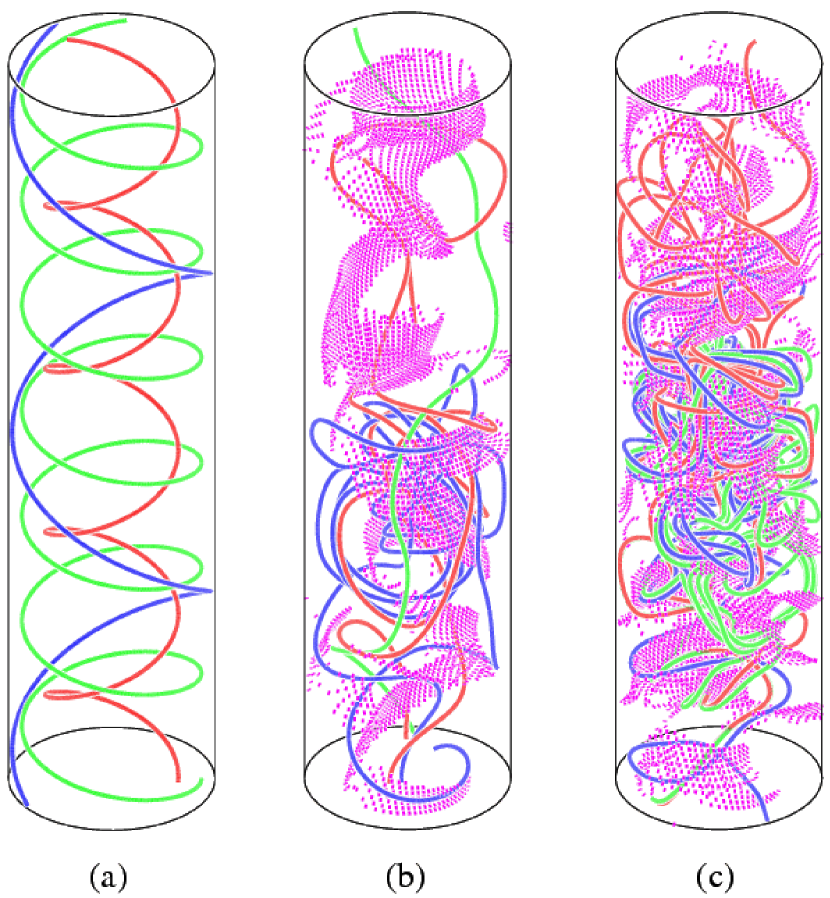
Figure 6.— Tangled magnetic fields obtained by superposition of modes of the linear force-free field inside a cylinder, which represents a vertical thread within a hedgerow prominence. The radial component of the field $B_{r}$ vanishes at the cylinder wall. The three panels show models with different values of $a\equiv|\alpha|R$, where $\alpha$ is the torsion parameter and $R$ is the cylinder radius: (a) $a=3.0$; (b) $a=4.5$ ; (c) $a=6.0$. In case (a) the field has only a single mode, but is cases (b) and (c) there are multiple modes ($N=4$ and $N=6$), some of which are non-axisymmetric, resulting in tangled field lines. Each panel shows three field lines (red, green and blue curves). In panels (b) and (c) the magenta dots show dips in the field lines.

5. Deviations from the Force-Free Condition

The above models for a tangled field are purely force-free and do not have any magnetic forces to support the prominence plasma against gravity. To include such effects, we now consider the “elastic” properties of the tangled field, i.e., its response to external forces. Specifically, the weight of the prominence causes the tangled field to be compressed in the vertical direction, resulting in a radially outward force on the plasma. Also, shearing motions may occur within the tangled field as dense plasma moves downward and less dense “plumes” move upward (e.g., Berger et al., 2008). This results in shear deformation of the tangled field and associated magnetic stresses that counteract the plasma flows. In the following both of these effects are considered in some detail.

5.1. Compressional Effect

We first consider the effects of gravity on a layer of tangled magnetic field. The magnetostatic equation ($-\nabla p+\rho{\bf g}+{\bf F}=0$) cannot be solved analytically for a tangled field, so we make the following approximation:

$${\bf B}^{\prime}({\bf r})\equiv\nabla\times\left[\frac{1}{\alpha}{\bf B}({\bf r})e^{-z/H_{B}}\right]=\left[{\bf B}({\bf r})-\frac{1}{\alpha H_{B}}\hat{\bf z}\times{\bf B}({\bf r})\right]e^{-z/H_{B}}.$$ (31)

Here ${\bf B}({\bf r})$ is the LFFF given by equation (15), and $H_{B}$ is the magnetic scale height of the modified field (we assume $|\alpha|H_{B}>2$). Note that $\nabla\cdot{\bf B}^{\prime}=0$ as required. This modified field ${\bf B}^{\prime}({\bf r})$ is no longer force-free, but has the following statistical properties:

$$<{\bf B}^{\prime}>=0,$$ (32)

$$<{\bf B}^{\prime}{\bf B}^{\prime}>=\text@frac{1}{3}B_{0}^{2}\left[(1+\epsilon^{2})(\hat{\bf x}\hat{\bf x}+\hat{\bf y}\hat{\bf y})+\hat{\bf z}\hat{\bf z}\right]e^{-2z/H_{B}},$$ (33)

where $\epsilon\equiv(|\alpha|H_{B})^{-1}<\text@frac{1}{2}$. Therefore, the magnitude of the modified field drops off exponentially with height $z$. Let $T_{ij}^{\prime}$ be the magnetic stress tensor of the modified field. Taking its statistical average, we find for the nonzero components of the stress tensor:

$$<T_{xx}^{\prime}>=<T_{yy}^{\prime}>=-\frac{B_{0}^{2}}{24\pi}~{}e^{-2z/H_{B}},$$ (34)

$$<T_{zz}^{\prime}>=-\frac{B_{0}^{2}}{24\pi}(1+2\epsilon^{2})~{}e^{-2z/H_{B}}.$$ (35)

Note that for $\epsilon<\text@frac{1}{2}$ the stress tensor is nearly isotropic. The net force on the plasma is given by $F_{i}^{\prime}=\partial T_{ij}^{\prime}/\partial x_{j}$, and the average force follows from equations (34) and (35):

$$<F_{x}^{\prime}> = <F_{y}^{\prime}>=0,$$ (36)

$$<F_{z}^{\prime}> = \frac{B_{0}^{2}}{12\pi H_{B}}(1+2\epsilon^{2})~{}e^{-2z/H_{B}}.$$ (37)

Note that the average force acts in the positive $z$ direction, i.e., the magnetic force counteracts the force of gravity. In effect, the plasma is being supported by the magnetic pressure of the tangled field. The tangled field acts like a hot gas that has a significant pressure but no mass. The average density of the plasma that can be supported by the tangled field is given by

$$\rho_{avg}(z)=\frac{<F_{z}^{\prime}>}{g}=\frac{B_{0}^{2}}{12\pi gH_{B}}~{}(1+2\epsilon^{2})~{}e^{-2z/H_{B}},$$ (38)

where $g$ is the acceleration of gravity.

The horizontal components of Lorentz force, $F_{x}^{\prime}$ and $F_{y}^{\prime}$, do not vanish for any particular realization of the tangled field, and cannot be written as the gradients of a scalar pressure $p$. The reason is that expression (31) is not an exact solution of the magnetostatic equilibrium equation. However, equation (36) shows that the horizontal forces vanish when averaged over the fluctuations of the isotropic tangled field. Therefore, expression (31) is thought to give a good approximation for the effects of gravity on the tangled field.

We now apply the above model to the vertical threads observed in hedgerow prominences. To explain the observed heights of such prominences, we require that the magnetic scale height $H_{B}$ is at least 100 Mm. The size $\ell$ of the magnetic tangles is assumed to be in the range 0.1–1 Mm, so $\epsilon=\ell/H_{B}\ll 1$. For $B_{0}=10$ G and $H_{B}=100$ Mm, we find $\rho_{avg}\approx 10^{-14}$ $\rm g~{}cm^{-3}$, which corresponds to an average (total) hydrogen density $n_{H,avg}\approx 5\times 10^{9}$ $\rm cm^{-3}$. This is only about 0.05 times the density $\rho_{0}\approx 2\times 10^{-13}$ $\rm g~{}cm^{-3}$ or $n_{H}\approx 10^{11}$ $\rm cm^{-3}$ typically observed in hedgerow prominences (Engvold, 1976, 1980; Hirayama, 1986). This comparison shows that the pressure of the tangled field inside a prominence thread is not sufficient to support the weight of the prominence plasma. To support the plasma with tangled fields, we need to take into account the magnetic coupling between the vertical thread and its surroudings. Such coupling is neglected in the above plane-parallel model.

5.2. Shear Stress Effect

We now assume that the tangled field pervades not only the observed vertical threads but also their local surroundings. The density in the surroundings is less than that in the threads, so the force of gravity is also much lower. This difference in gravitational forces leads to vertical motions (downflows in the dense threads, upflows in the tenuous surroundings) that create magnetic stresses in the tangled field. The magnetic coupling between the prominence and its surroundings causes the weight of the dense prominence to be distributed over a wider area. In effect, the prominence plasma is being supported by the radial gradient of the magnetic pressure of the tangled field over this larger area. In the following we estimate the magnetic stresses and vertical displacements resulting from these forces.

The tangled field is modeled either as a vertical slab with half-width $R$, or as a vertical cylinder with radius $R$. The prominence is located at the center of this slab or cylinder, and has a half-width or radius $r_{0}<R$. Then the average density in the tangled field region is given by

$$\rho_{avg}\approx\rho_{0}\left(\frac{r_{0}}{R}\right)^{n},$$ (39)

where $\rho_{0}$ is the density of the prominence, and we neglect the mass of the surroundings. The exponent $n=1$ for the slab model or $n=2$ for the cylindrical model. As discussed in Section 5.1, observations of hedgerow prominences indicate $\rho_{0}\approx 2\times 10^{-13}$ $\rm g~{}cm^{-3}$ (e.g., Engvold, 1976), and to explain the observed heights of such prominences with $B_{0}=10$ G, we require $\rho_{avg}/\rho_{0}<0.05$. According to equation (39), this implies $R/r_{0}\geq 20$ for the slab model, or $R/r_{0}\geq 4.5$ for the cylindrical model. The observed threads have widths down to about 500 km (Engvold, 1976), which corresponds to $r_{0}\approx 250$ km. Therefore, the magnetic coupling by the tangled field must extend to a surrounding distance of at least 5 Mm for the slab model, or 1.1 Mm for the cylindrical model. More generally, equations (38) and (39) yield the following expression for the magnetic scale height of tangled field:

$$H_{B}\approx\frac{B_{0}^{2}}{12\pi g\rho_{0}}\left(\frac{R}{r_{0}}\right)^{n}.$$ (40)

Therefore, the maximum height of the prominence depends strongly on the magnetic field strength $B_{0}$.

According to the present model, magnetic stress builds up in the tangled field as a result of the difference in gravitational forces between the thread and its surroundings. Can the field support such shear stress? To answer this question we examine the effect of vertical displacements on the tangled field. For simplicity we neglect the mean vertical force given by equation (37), and we focus on relative displacements. Let ${\bf r}^{\prime}$ be the new position of a fluid parcel originally located at position ${\bf r}$. In the limit of a perfectly conducting plasma, the deformed field ${\bf B}^{\prime}$ at the new position ${\bf r}^{\prime}$ is given by

$$B_{i}^{\prime}=\frac{B_{j}}{J}\frac{\partial x_{i}^{\prime}}{\partial x_{j}},$$ (41)

where ${\bf B}({\bf r})$ is the original field, and $J$ is the Jacobian of the transformation (e.g., Priest, 1982). We assume

$$x^{\prime}=x,~{}~{}~{}~{}y^{\prime}=y,~{}~{}~{}~{}z^{\prime}=z+h(x,y),$$ (42)

which yields

$$B_{x}^{\prime}=B_{x},~{}~{}~{}~{}B_{y}^{\prime}=B_{y},~{}~{}~{}~{}B_{z}^{\prime}=B_{z}+B_{x}\frac{\partial h}{\partial x}+B_{y}\frac{\partial h}{\partial y},$$ (43)

where $h(x,y)$ is the vertical displacement. The original field ${\bf B}({\bf r})$ is assumed to be a realization of the isotropic tangled field given by equation (15). Using equation (22), we obtain

$$<{\bf B}^{\prime}>=0,$$ (44)

$$<{\bf B}^{\prime}{\bf B}^{\prime}>=\text@frac{1}{3}B_{0}^{2}\left[\hat{\bf x}\hat{\bf x}+\hat{\bf y}\hat{\bf y}+f\hat{\bf z}\hat{\bf z}+\frac{\partial h}{\partial x}\hat{\bf x}\hat{\bf z}+\frac{\partial h}{\partial y}\hat{\bf y}\hat{\bf z}\right],$$ (45)

where

$$f(x,y)\equiv 1+\left(\frac{\partial h}{\partial x}\right)^{2}+\left(\frac{\partial h}{\partial y}\right)^{2}.$$ (46)

This yields the following expressions for the off-diagonal components of the stress tensor:

$$<T_{xz}^{\prime}>=\frac{B_{0}^{2}}{12\pi}\frac{\partial h}{\partial x},~{}~{}~{}~{}<T_{yz}^{\prime}>=\frac{B_{0}^{2}}{12\pi}\frac{\partial h}{\partial y}.$$ (47)

The Lorentz force is given by $F_{i}^{\prime}=\partial T_{ij}^{\prime}/\partial x_{j}$, and since $<T_{zz}^{\prime}>$ is independent of $z$, the average vertical force is given by

$$<F_{z}^{\prime}>=\frac{B_{0}^{2}}{12\pi}\left(\frac{\partial^{2}h}{\partial x^{2}}+\frac{\partial^{2}h}{\partial y^{2}}\right)=g\Delta\rho(x,y),$$ (48)

where $\Delta\rho(x,y)$ is the density perturbation ($\Delta\rho\equiv\rho-\rho_{avg}$). Using this equation, we can determine the vertical displacement $h(x,y)$ for a given density variation $\Delta\rho(x,y)$. In the following subsections we solve the above equation for the slab and cylinder models.

5.2.1 Slab Model

We first consider a slab with infinite extent in the $+y$, $-y$ and $+z$ directions. The coordinate $x$ perpendicular to the slab is in the range $-R<x<R$, where $R$ is the half-width of the sheet in which the tangled field is embedded (see Figure 2b). Then the density perturbation is given by

$$\Delta\rho(x)=\left\{\begin{array}[]{ll}+\rho_{0}[1-(r_{0}/R)]&\mbox{for}~{}|x|<r_{0},\\ -\rho_{0}r_{0}/R&\mbox{otherwise}.\end{array}\right.$$ (49)

Inserting this expression into equation (48) and solving for the vertical displacement, we obtain

$$h(x)=\left\{\begin{array}[]{ll}C[1-(r_{0}/R)](x^{2}-r_{0}^{2})&\mbox{for}~{}|x|<r_{0},\\ C(r_{0}/R)[(R-r_{0})^{2}-(R-|x|)^{2}]&\mbox{otherwise},\end{array}\right.$$ (50)

where $C\equiv 6\pi g\rho_{0}B_{0}^{-2}$. Here we applied no-stress boundary conditions ($dh/dx=0$) at $x=\pm R$. Note that $h(x)$ and its derivative are continuous at the edges of the prominence ($x=\pm r_{0}$). The relative displacement across the tangled field is given by

$$\Delta h\equiv h(R)-h(0)=\frac{6\pi g\rho_{0}}{B_{0}^{2}}r_{0}(R-r_{0}).$$ (51)

Figure 7a shows the function $h(x)$ for $r_{0}=0.5$ Mm, $R=10$ Mm, $B_{0}=10$ G and $\rho_{0}=2\times 10^{-13}$ $\rm g~{}cm^{-3}$, so that $\Delta h=0.491$ Mm. Note that a relatively small deformation of the tangled field ($\Delta h\ll R$) is sufficient to redistribute the gravitational forces over the full width of the tangled field. However, $\Delta h$ is larger than the pressure scale height of the prominence plasma ($H_{p}\approx 0.2$ Mm). Therefore, the deformation of the tangled field in the neighborhood of the prominence may have a significant effect on the distribution of the prominence plasma. This issue will be further discussed in Section 7.

Figure 7.— Vertical displacements in the tangled magnetic field supporting a hedgerow prominence. (a) Slab model with $R=10$ Mm, $r_{0}=0.5$ Mm, and $B_{0}=10$ G. The vertical displacement $h(x)$ is plotted as function of position $x$ perpendicular to the vertical slab. The location of the prominence is indicated by the dotted lines. (b) Cylindrical model of a prominence thread with $R=5$ Mm, $r_{0}=1$ Mm, and $B_{0}=3$ G. In both cases the prominence density $\rho_{0}=2\times 10^{-13}$ $\rm g~{}cm^{-3}$.

For comparison of the tangled field slab model with the flux rope model (Figure 2), we define the average sag angle $\theta$ of the prominence relative to its surroundings:

$$\tan\theta\equiv\frac{\Delta h}{R}\approx\frac{6\pi g\rho_{0}r_{0}}{B_{0}^{2}},$$ (52)

where $B_{0}$ is the r.m.s. field strength of the tangled field, and we assumed $r_{0}\ll R$. This expression is similar to that derived for the Kippenhahn-Schlüter model:

$$\tan\theta=\frac{4\pi g\rho_{0}r_{0}}{B_{x}^{2}},$$ (53)

where $B_{x}$ is the magnetic field through the mid-plane of the prominence (Kippenhahn & Schlüter, 1957). Equation (53) describes the angle of the field lines in the flux rope model shown in Figure 2a. Therefore, the flux-rope and tangled field models are similar in their ability to explain the magnetic support of the prominence plasma, provided the half-width $R$ of the tangled field region is similar to the radius $R$ of the flux rope.

5.2.2 Cylindrical Model

We now consider a cylindrical model for a prominence thread with $r$ the distance from the (vertical) thread axis. The density perturbation is given by

$$\Delta\rho(r)=\left\{\begin{array}[]{ll}+\rho_{0}[1-(r_{0}/R)^{2}]&\mbox{for}~{}r<r_{0},\\ -\rho_{0}(r_{0}/R)^{2}&\mbox{for}~{}r_{0}<r<R.\end{array}\right.$$ (54)

The vertical displacement is obtained by solving equation (48), which yields

$$h(r)=\left\{\begin{array}[]{ll}h_{0}[(r/r_{0})^{2}-1]&\mbox{for}~{}r<r_{0},\\ h_{0}[2R^{2}\ln(r/r_{0})-r^{2}+r_{0}^{2}]/(R^{2}-r_{0}^{2})&\mbox{for}~{}r_{0}<r<R,\end{array}\right.$$ (55)

where

$$h_{0}\equiv\frac{3\pi}{B_{0}^{2}}g\rho_{0}r_{0}^{2}\left(1-\frac{r_{0}^{2}}{R^{2}}\right),$$ (56)

and we applied no-stress boundary conditions at $r=R$. Then the total displacement across the tangled field is

$$\Delta h\equiv h(R)-h(0)=\frac{6\pi g\rho_{0}}{B_{0}^{2}}r_{0}^{2}\ln\left(\frac{R}{r_{0}}\right).$$ (57)

Figure 7b shows the vertical displacement $h(r)$ for $R=5$ Mm, $r_{0}=1$ Mm, $B_{0}=3$ G and $\rho_{0}=2\times 10^{-13}$ $\rm g~{}cm^{-3}$, which yields $h_{0}=0.551$ Mm and $\Delta h=1.847$ Mm. In this case $\Delta h$ is significantly larger than the pressure scale height ($H_{p}\approx 0.2$ Mm), mainly because of the lower field strength compared to the case shown in Figure 7a. In Section 7 we consider the effect of such deformation on the field-line dips, and on the spatial distribution of the prominence plasma.

The above analyses only provide an rough estimate for the density of prominence plasma that can be supported by the tangled field. The actual density distribution $\rho({\bf r},t)$ is likely to be much more complex for several reasons. First, plasma will tend to collect at the dips of the field lines, so the density will vary on the spatial scale $\ell$ of the tangled field and on the scale of $H_{p}$; this effect will be considered in more detail in Section 7. Second, the density will vary with time because there are flows along the field lines (see Section 3) and these flows are likely to be non-steady. Also, the magnetic structure is not fixed and will continually evolve as dipped field lines are distorted by the weight of the prominence plasma. To predict the actual density will require numerical simulations of the interaction of tangled fields with prominence plasma, which is beyond the scope of the present paper.

6. Formation of Vertical Threads by Rayleigh-Taylor Instability

According to the present theory, hedgerow prominences are supported by the pressure of a tangled magnetic field, which acts like a tenuous gas and is naturally buoyant. It is well known that a tenuous medium supporting a dense medium is subject to Rayleigh-Taylor (RT) instability (Chandrasekhar, 1961). Therefore, we suggest that the observed vertical threads may be a consequence of RT instability acting on the tangled field and the plasma contained within it. As cool plasma collects in certain regions of the tangled field, the weight of the plasma deforms the surrounding field, which causes even more plasma to flow into these regions.

A detailed analysis of the formation of prominence threads by RT instability is complicated by the fact that we presently do not understand how a tangled field responds to shear deformation. In Section 5.2 we estimated the relative vertical displacement $\Delta h$ of the prominence plasma assuming no reconnection occurs during the deformation of the magnetic field by gravity forces [see equations (51) and (57)]. In this case the tangled field behaves as an “elastic” medium with magnetic forces proportional to the displacement. However, it is not clear that this approximation is valid. High-resolution observations of prominences indicate that the dense threads move downward relative to their more tenuous surroundings with velocities of the order of 10-30 $\rm km~{}s^{-1}$ (e.g., Berger et al., 2008; Chae et al., 2008). If the threads and their surroundings are indeed coupled via tangled fields, these relative motions imply that the field is continually being stretched in the vertical direction. Therefore, the shear stress continually increases with time, unless there is internal reconnection that causes the shear stress to be reduced.

We speculate that tangled fields have a tendency to relax to the LFFF via internal reconnection. A similar relaxation processes occurs in the reversed field pinch and other laboratory plasma physics devices (Taylor, 1974). Therefore, the long-term evolution of prominence threads likely involves small-scale reconnection within the tangled field. The tangled field may behave more like a “plastic” medium that is irreversibly deformed when subjected to shear stress. Such plasticity makes it possible to understand how the dense threads can move downward relative their the surroundings at a small but constant speed. These flows significantly deform the tangled field, but the field is nevertheless able to support the plasma against gravity. A detailed analysis of reconnection in tangled fields and its effect on the prominence plasma is beyond the scope of the present paper.

The observed vertical structures likely reflect the non-linear development of the RT instability in hedgerow prominences. To establish a vertical column of mass resembling a prominence thread will likely require vertical motions over a significant height range (tens of Mm). Starting from a homogeneous density distribution, it may take several hours for the threads to form by RT instability.

7. Model for a Prominence Thread

We now construct a model for the density distribution in a fully formed (vertical) prominence thread supported by a tangled field. It is assumed that the RT instability has produced a vertical thread that is clearly separated from the rest of the prominence plasma. Therefore, only a single thread and its local surroundings are considered, and the tangled field is assumed to be contained in a vertical cylinder with radius $R=5$ Mm. As discussed in Section 3, there will in general be mass flows along the tangled field lines, but for the purpose of the present model we neglect such flows and we assume that the plasma is in hydrostatic equilibrium along the field lines.

To construct the density model, we first compute a particular realization of the LFFF with $\alpha R=9$ (see Appendix for details). To account for the weight of the prominence plasma, this field is further deformed as described by equation (55). The deformation parameters are $r_{0}=1.25$ Mm and $h_{0}=1.5$ Mm, which yields $\Delta h=4.44$ Mm, somewhat larger than the values used in Figure 7b. As shown in Section 5.1, the weight of the prominence plasma causes the strength of the tangled field to decrease with height [see equation (31)], but for simplicity this gradient is neglected here. The pressure scale height is assumed to be constant, $H_{p}=0.2$ Mm, which corresponds to a temperature of about 8000 K, typical for H$\alpha$ emitting plasma in prominences.

Figure 8.— Height $z(s)$ as function of position $s$ along a field line in the cylindrical tangled field model with $a=9.0$. Lengths are in units of the cylinder radius $R$.

We introduce cartesian coordinates $(x,y,z)$ with the $z$ axis along the cylinder axis; the $x$ and $y$ coordinates are in the range $[-R,+R]$, and the height $z$ is in the range $[0,10R]$. The density $\rho(x,y,z)$ in this volume is computed on a grid with $200\times 200\times 1000$ grid points, using the following method. We randomly select a large number of points within the cylinder and trace out the field lines that pass through these points. For each field line we plot the height $z(s)$ as function of position $s$ along the field line, and we find the peaks and dips in the field line. For each dip we find the two neighboring peaks ($s_{1}$ and $s_{2}$) and we determine the depth $\Delta z$ of the valley between these peaks. We then iteratively remove shallow dips with $\Delta z<3H_{p}$ by concatenating neighboring sections. Figure 8 shows an example for one particular field line; the remaining dips with $\Delta z>3H_{p}$ are indicated by squares. We then compute the density $\rho(s)$ in each interval, assuming hydrostatic equilibrium along the field line [see equation (10)]. Since we are interested only in relative densities, we set $\rho_{dip}=1$, the same for all dips on all field lines. Finally, we distribute the density $\rho(s)$ onto the 3D grid by finding the grid points that lie closest to the path of the field line. This process is repeated for 8000 field lines to obtain the density $\rho(x,y,z)$ throughout the 3D grid.

Figure 9 shows the resulting density distribution. The three panels show different projections obtained by integration in the $x$, $y$ and $z$ directions, respectively [for example, Figure 9a shows $\int\rho(x,y,z)dx$]. Note that the plasma is concentrated in the central part of the cylinder; this is due to the deformation of the magnetic field described by the vertical displacement $h(r)$, which changes the distribution of the field-line dips compared to that in the LFFF. The plasma is highly inhomogenous ($\rho_{max}\approx 50\rho_{avg}$), and is distributed in sheets corresponding to surfaces of field-line dips. In some regions there are multiple sheets along the line of sight (LOS). This is consistent with observations of the H I Lyman lines in solar prominences, which indicate multiple threads along the LOS (Orrall & Schmahl, 1980; Gunár et al., 2007).

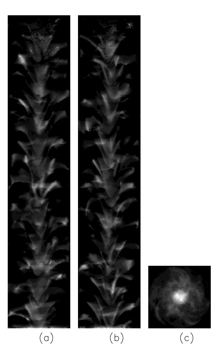
Figure 9.— Simulated density distribution of a prominence thread. The thread is supported by a tangled magnetic field with $R=5$ Mm and $\alpha R=9$. The field is distorted by the weight of the prominence plasma ($r_{0}=1.25$ Mm, $h_{0}=1.5$ Mm). The plasma is concentrated at the dips of the tangled field lines. The density distribution along the field lines assumes hydrostatic equilibrium with $H_{p}=0.2$ Mm. The three panels show the column density distributions as seen from the $x$, $y$ and $z$ directions, respectively. Note that multiple sheets of plasma are superposed along the line of sight.

The above model is quasi-static and does not take into account the expected mass flows along the field lines (Section 3), nor the dynamical processes by which the threads are formed (Section 6). Constructing a more realistic 3D dynamical model of a prominence thread supported by tangled fields is beyond the scope of the present paper. However, our main conclusion that the density distribution within the thread is highly inhomogeneous is likely to be valid also in the dynamical case.

8. Summary and Discussion

We propose that hedgerow prominences are supported by magnetic fields that are “tangled” on a spatial scale of 1 Mm or less. A key feature of the model is that the plasma is approximately in magnetostatic balance, therefore, the model is different from earlier models in which the plasma is supported by MHD-wave pressure (e.g., Jensen, 1983, 1986; Pecseli & Engvold, 2000). In the present case the perturbations of the magnetic field do not propagate along the field lines. The tangled field is located within a large-scale current sheet standing vertically above the PIL (Figure 2b), and is not magnetically connected to the photosphere on either side of the PIL. Such tangled fields may be formed by flux emergence followed by magnetic reconnection in the low corona.

In this paper we use a variety of methods to explore the interactions of prominence plasma with tangled fields. In Section 3 a simple model for the downward flow of plasma along the distorted field lines was developed. It was shown that such flows naturally develop standing shocks where the gravitational energy of the plasma is converted into heat; this may be important for understanding the heating of prominence plasmas. The average flow velocity is less than the sound speed, indicating that the tangled field is able to support the prominence plasma against gravity.

In Section 4 linear force-free models of tangled fields were constructed. Tangled fields can be described as a superposition of planar modes. We studied the statistical properties of such fields, and found random-walk behavior of the field lines when the number of modes is sufficiently large ($N>10$). To produce tangling of the field lines on a scale of 1 Mm or less, as required for our model of hedgerow prominences, we need $|\alpha|>1$ $\rm Mm^{-1}$, much larger than the values typically found in measurements of photospheric vector fields. Therefore, according to the present model, hedgerow prominences are embedded in magnetic fields with high magnetic helicity density. We also considered the conditions for confinement of a tangled field by the surrounding smooth fields, and showed that despite the high helicity density tangled fields can be in pressure balance with their surroundings.

In Section 5 the “elastic” properties of a tangled field were considered, i.e., their linear response to gravitational forces assuming ideal MHD. We found that the weight of the prominence plasma can be supported by the nearly isotropic magnetic pressure of the tangled field. The tangled field pervades not only the observed vertical threads, but also their local surroundings. The magnetic coupling between the threads and their surroundings is quite strong: vertical displacements of only 0.5–2 Mm are sufficient to counteract the shear stress resulting from the different gravitational forces. In effect, the weight of a dense thread is distributed over an area that is larger than the cross-sectional area of the thread. As discussed in Section 5.2, the observed densities in prominence threads ($n_{H}\sim 10^{11}$ $\rm cm^{-3}$) can be supported by tangled fields with field strengths in the range 3–15 G.

In Section 6 we proposed that the observed vertical structures in hedgerow prominences are a consequence of Rayleigh-Taylor (RT) instability acting on the tangled field and the plasma contained within it. The tangled field acts like a hot, tenuous gas and is naturally buoyant; its support of the dense prominence plasma is likely to be unstable to flows that separate the gas into dense and less-dense columns. The observed vertical structures likely reflect the non-linear development of the RT instability. A detailed analysis of this instability is complicated by the fact that it requires internal reconnection to occur within the tangled field, and it is unclear how rapidly such reconnection can proceed. Therefore, it is difficult to predict the vertical velocities in prominence threads. Clearly, more advanced numerical simulations of the interaction of tangled fields with prominence plasma are needed.

Finally, in Section 7 we simulated the density distribution in a prominence thread, using a cylindrical model for the tangled field and its deformation by gravitational forces. The results indicate that the threads have an intricate fine-scale structure. Multiple structures are superposed along the LOS, consistent with observations of the H I Lyman lines (Orrall & Schmahl, 1980; Gunár et al., 2007). While our model does not take into account any dynamical processes, the main conclusion that the density distribution is highly inhomogeneous is likely to be valid also in the dynamical case.

Appendix A Tangled Fields in a Cylinder

According to the model presented in this paper, the vertical threads in hedgerow prominences are supported by tangled magnetic fields that pervade the dense threads and their local surroundings. In this section we construct a cylindrical model of this tangled field. We use a cylindrical coordinate system $(r,\phi,z)$ with $r$ the distance from the cylinder axis ($r\leq R$ where $R$ is the cylinder radius), $\phi$ the azimuthal angle, and $z$ the height along the axis. We assume that the radial component of the field vanishes at the cylinder wall, $B_{r}(R,\phi,z)=0$, so the field lines are confined to the interior of the cylinder. It follows that the axial magnetic flux must be constant along the cylinder:

$$\Phi\equiv\int_{0}^{R}\int_{0}^{2\pi}B_{z}(r,\phi,z)r~{}dr~{}d\phi=\hbox{constant}.$$ (A1)

In cylindrical coordinates the force-free condition reads:

$$\frac{1}{r}\frac{\partial B_{z}}{\partial\phi}-\frac{\partial B_{\phi}}{\partial z} = \alpha B_{r},$$ (A2)

$$\frac{\partial B_{r}}{\partial z}-\frac{\partial B_{z}}{\partial r} = \alpha B_{\phi},$$ (A3)

$$\frac{1}{r}\frac{\partial}{\partial r}\left(rB_{\phi}\right)-\frac{1}{r}\frac{\partial B_{r}}{\partial\phi} = \alpha B_{z}.$$ (A4)

We again take $\alpha$ to be constant (LFFF). The general solution of the above equations with the boundary condition $B_{r}(R,\phi,z)=0$ can be written as a superposition of discrete eigenmodes enumerated by an index $n$:

$$B_{r}(r,\phi,z) = \sum_{n=1}^{N}\tilde{B}_{n}F_{r,n}(r)\sin(k_{n}z+m_{n}\phi+f_{n}),$$ (A5)

$$B_{\phi}(r,\phi,z) = \sum_{n=1}^{N}\tilde{B}_{n}F_{\phi,n}(r)\cos(k_{n}z+m_{n}\phi+f_{n}),$$ (A6)

$$B_{z}(r,\phi,z) = \sum_{n=1}^{N}\tilde{B}_{n}F_{z,n}(r)\cos(k_{n}z+m_{n}\phi+f_{n}),$$ (A7)

where $\tilde{B}_{n}$ is the mode amplitude; the functions $F_{r,n}(r)$, $F_{\phi,n}(r)$ and $F_{z,n}(r)$ describe the radial dependence of each mode; $k_{n}$ is the axial wavenumber; $m_{n}$ is the azimuthal wavenumber (non-negative integer); and $f_{n}$ is the phase. Here $n=1$ refers to a fully symmetric mode with $k_{1}=m_{1}=f_{1}=0$ (also known as the Lundquist mode), while $n=2,\cdots,N$ refers to modes that have either a $\phi$ or $z$ dependence. The latter modes only exist under certain conditions (see below). Inserting expressions (A5), (A6) and (A7) into equations (A2), (A3) and (A4), we find that the radial dependencies can be expressed in terms of Bessel functions:

$$F_{r,n}(r) = -\frac{k_{n}}{q_{n}}J_{m}^{\prime}(q_{n}r)-\frac{\alpha m_{n}}{q_{n}^{2}r}J_{m}(q_{n}r),$$ (A8)

$$F_{\phi,n}(r) = -\frac{\alpha}{q_{n}}J_{m}^{\prime}(q_{n}r)-\frac{k_{n}m_{n}}{q_{n}^{2}r}J_{m}(q_{n}r),$$ (A9)

$$F_{z,n}(r) = J_{m}(q_{n}r),$$ (A10)

where $q_{n}\equiv\sqrt{\alpha^{2}-k_{n}^{2}}$ is the radial wavenumber, $J_{m}(x)$ is the Bessel function of order $m_{n}$, and $J_{m}^{\prime}(x)$ is its derivative. The boundary condition at the cylindrical wall requires $F_{r,n}(R)=0$ for all modes. Introducing a parameter $\theta_{n}$ in the range $[0,\pi]$ such that $q_{n}=|\alpha|\sin\theta_{n}$ and $k_{n}=\alpha\cos\theta_{n}$, we obtain the following equation for $\theta_{n}$:

$$\cos\theta_{n}J_{m}^{\prime}(a\sin\theta_{n})+\frac{m_{n}}{a\sin\theta_{n}}J_{m}(a\sin\theta_{n})=0,$$ (A11)

where $a\equiv|\alpha|R$. The roots of this equation can be found numerically for any given values of $a$ and $m$. Depending on the value of $a$, the equation may have one or more solutions:

1. There always exists at least one solution, the axisymmetric mode ($m_{1}=0$) with $\theta_{1}=\pi/2$. In this case $q_{1}=|\alpha|$ and $k_{1}=0$, so this mode is invariant with respect to translation along the $z$ axis (Lundquist mode).

2. There may be additional axisymmetric modes that are not invariant to translation. In the case $m_{n}=0$ and $\theta_{n}\neq\pi/2$, equation (A11) yields $a\sin\theta_{n}=x_{i}$, where $x_{i}$ is a root of $J_{0}^{\prime}(x)=0$ ($x_{1}=3.832$, $x_{2}=7.016$, $x_{3}=10.173$, etc.). Solutions exist only when $a>x_{1}$; for $a$ in the range $[x_{1},x_{2}]$ there exists one such solution with $\theta_{n}=\arcsin(x_{1}/a)$; for $a$ in the range $[x_{2},x_{3}]$ there exist two solution, etc. Since $J_{0}^{\prime}(a\sin\theta)$ is symmetric with respect to $\theta=\pi/2$, each solution $\theta_{n}$ also has a second solution $\theta_{n}^{\prime}=\pi-\theta_{n}$, but the magnetic structure of these solutions is the same, so we do not count it as a separate mode.

3. For higher values of $a$ there exist non-axisymmetric solutions ($m_{n}\geq 1$). The first modes with $m=1$ occur at $a=3.112$; these “kink” modes are apparently more easily excited than the axisymmetric modes with $k\neq 0$. The first modes with $m=2$ occur at $a=4.708$.

For a given value of $a$, we systematically find all roots of equation (A11), starting with $m=0$ and then increasing $m$ until no more roots are found. Figure 10 shows $\theta_{n}$ as function of $a$. Note that the number of modes $N$ increases with $a$.

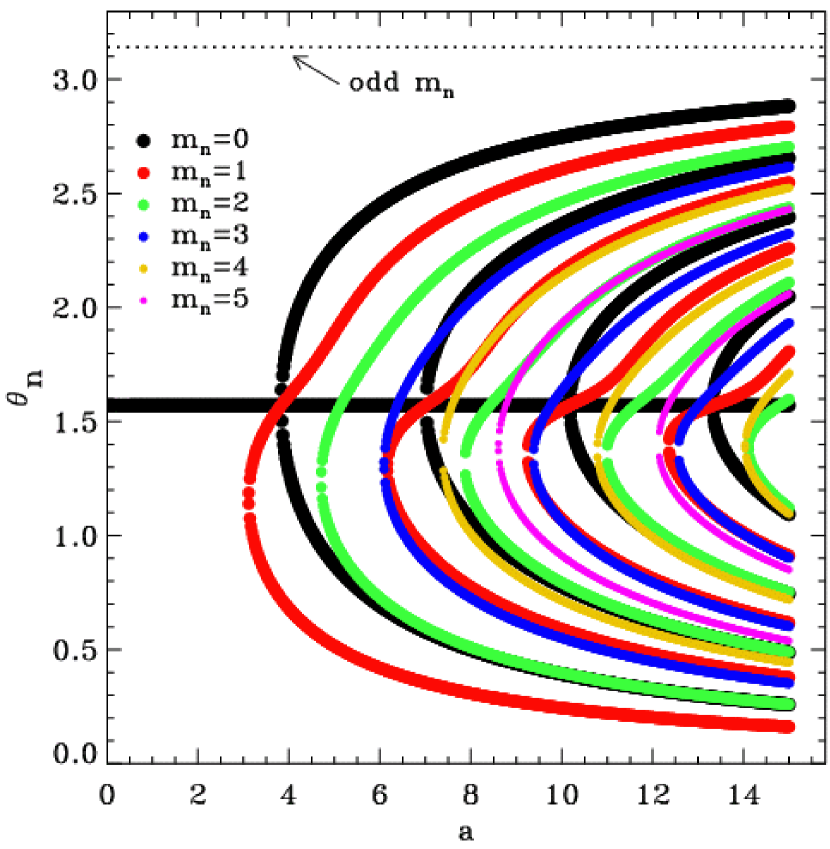
Figure 10.— Modes of the tangled field in a cylinder (see text for details).

We now compute the axial flux and magnetic energy density. Inserting equations (A7) and (A10) into equation (A1), we find that only the Lundquist mode contributes to the axial magnetic flux:

$$\Phi=2\pi\tilde{B}_{1}\int_{0}^{R}J_{0}(|\alpha|r)r~{}dr=2\pi R\tilde{B}_{1}|\alpha|^{-1}J_{1}(a).$$ (A12)

where we used $J_{0}^{\prime}(q_{n}R)=0$ for axisymmetric modes. The mean magnetic energy density is defined by

$$E\equiv\frac{2}{R^{2}}\int_{0}^{R}\left\langle\frac{B^{2}}{8\pi}\right\rangle~{}r~{}dr,$$ (A13)

where $<\cdots>$ denotes an average over $\phi$ and $z$. Let $n1$ and $n2$ denote two different modes, then averages of cross products such as $<\cos(k_{n1}z+m_{n1}\phi+f_{n1})$ $\cos(k_{n2}z+m_{n2}\phi+f_{n2})>$ vanish. Therefore, the magnetic energy can be written as a sum over individual modes, $E=\sum_{n=1}^{N}E_{n}$, where

$$E_{1} = \frac{\tilde{B}_{1}^{2}}{4\pi R^{2}}\int_{0}^{R}\left[J_{0}^{2}(|\alpha|r)+J_{1}^{2}(|\alpha|r)\right]r~{}dr,$$ (A14)

$$E_{n} = \frac{\tilde{B}_{n}^{2}}{8\pi R^{2}}\int_{0}^{R}\left[F_{r,n}^{2}(r)+F_{\phi,n}^{2}(r)+F_{z,n}^{2}(r)\right]r~{}dr~{}~{}~{}~{}~{}\mbox{for}~{}n>1.$$ (A15)

For simplicity we consider equipartition tangled fields in which the various modes $n$ of the LFFF have equal magnetic energy. This implies $E_{n}=E/N$, the same for all modes (including the Lundquist mode), which provides a relationship between the mode amplitudes $\tilde{B}_{n}$. The phase angles $f_{n}$ of the non-axisymmetric modes are assigned random values in the range $[0,2\pi]$. This results in a tangled magnetic field ${\bf B}({\bf r})$ described by equations (A5), (A6) and (A7).

References

- Antiochos et al. (1999) Antiochos, S. K., MacNiece, P. J., Spicer, D. S., & Klimchuk, J. A. 1999, ApJ, 512, 985
- Aulanier et al. (1998) Aulanier, G., Démoulin, P., van Driel-Gesztelyi, L., Mein, P., & DeForest, C. 1998, A&A, 335, 309
- Berger et al. (2008) Berger, T. E., Shine, R. A., Slater, G. L., Tarbell, T. D., Title, A. M., Okamoto, T. J., Ichimoto, K., et al. 2008, ApJ, 676, L89
- Bommier & Leroy (1998) Bommier, V., & Leroy, J.-L. 1998, in New Perspectives on Solar Prominences, IAU Colloq. 167, eds. D. Webb, D. Rust, B. Schmieder. ASP Conf. Series, vol. 150 (Astron. Soc. of the Pacific, San Francisco), p. 434
- Casini et al. (2003) Casini, R., López Ariste, A., Tomczyk, S., & Lites, B. W. 2003, ApJ, 598, 67
- Casini, Bevilacqua & López Ariste (2005) Casini, R., Bevilacqua, R., & López Ariste, A. 2005, ApJ, 622, 1265
- Casini, Manso Sainz & Low (2009) Casini, R., Manso Sainz, R., & Low, B. C. 2009, ApJ, 701, L43
- Chae et al. (2008) Chae, J., Ahn, K., Lim, E.-K., Choe, G. S., & Sakurai, T. 2008, ApJ, 689, L73
- Chae et al. (2001) Chae, J., Wang, H., Qiu, J., Goode, P.R., Strous, L., & Yun, H.S. 2001, ApJ, 560, 476
- Chandrasekhar (1961) Chandrasekhar, S. 1961, Hydrodynamic and hydromagnetic stability (Oxford University Press), Chapter 10
- Close et al. (2005) Close, R. M., Parnell, C. E., Longcope, D. W., & Priest, E. R. 2005, Sol. Phys., 231, 45
- Cranmer (2004) Cranmer, S. R. 2004, Am. J. Phys., 72, 1397
- Dahlburg, Antiochos & Klimchuk (1998) Dahlburg, R. B., Antiochos, S. K., & Klimchuk, J. A. 1998, ApJ, 495, 485
- Dudik et al. (2008) Dudik, J., Aulanier, G., Schmieder, B., Bommier, V., & Roudier, T. 2008, Sol. Phys., 248, 29
- Engvold (1976) Engvold, O. 1976, Sol. Phys., 49, 283
- Engvold (1980) Engvold, O. 1980, Sol. Phys., 67, 351
- Gibson & Fan (2006) Gibson, S. E., & Fan, Y. 2006, J. Geophys. Res., 111, Issue A12, CiteID A12103
- Gunár et al. (2007) Gunár, S., Heinzel, P., Schmieder, B., Schwartz, P., & Anzer, U. 2007, A&A, 472, 929
- Hagenaar, Schrijver & Title (2003) Hagenaar, H. J., Schrijver, C. J., & Title, A. M. 2003, ApJ, 584, 1107
- Hagenaar, DeRosa & Schrijver (2008) Hagenaar, H. J., DeRosa, M. L., & Schrijver, C. J. 2008, ApJ, 678, 541
- Heinzel, Anzer & Gunár (2005) Heinzel, P., Anzer, U., & Gunár, S. 2005, A&A, 442, 331
- Heinzel (2007) Heinzel, P. 2007, in Proc. Coimbra Meeting, ASP Conf. Series, 368, 271
- Heinzel et al. (2008) Heinzel, P., Schmieder, B., Farnik, F., Schwartz, P., Labrosse, N., Kotrc, P., Anzer, U., et al. 2008, ApJ, 686, 1383
- Hirayama (1985) Hirayama, T. 1985, Sol. Phys., 100, 415
- Hirayama (1986) Hirayama, T. 1986, in Coronal and Prominence Plasmas, ed. A. I. Poland, NASA Conf. Publ. 2442, p. 149
- Howard et al. (2007) Howard, R. A., et al. 2007, Space Sci. Rev., 136, 67
- Jackson (1999) Jackson, J. D. 1999, Classical Electrodynamics, 3rd edition (John Wiley & Sons, Inc.), p. 193
- Jensen (1983) Jensen, E. 1983, Sol. Phys., 89, 275
- Jensen (1986) Jensen, E. 1986, in Coronal and Prominence Plasmas, ed. A. I. Poland, NASA Conf. Publ. 2442, p. 63
- Karpen & Antiochos (2008) Karpen, J. T., & Antiochos, S. K. 2008, ApJ, 676, 658
- Karpen, Antiochos & Klimchuk (2006) Karpen, J. T., Antiochos, S. K., & Klimchuk, J. A. 2006, ApJ, 637, 531
- Karpen et al. (2005) Karpen, J. T., Tanner, S. E. M., Antiochos, S. K., & DeVore, C. R. 2005, ApJ, 635, 1319
- Kippenhahn & Schlüter (1957) Kippenhahn, R. & Schlüter, A. 1957, Zeitschrift für Astrophysik, 43, 36
- Kucera, Tovar & De Pointieu (2003) Kucera, T. A., Tovar, M., De Pontieu, B. 2003, Sol. Phys., 212, 81
- Kuperus & Tandberg-Hanssen (1967) Kuperus, M. & Tandberg-Hanssen, E. 1967, Sol. Phys., 2, 39
- Kuperus & Raadu (1974) Kuperus, M., & Raadu, M. A. 1974, A&A, 31, 189
- Landau & Lifshitz (1959) Landau, L. D., & Lifshitz, E. M. 1959, Fluid Mechanics (Pergamon Press, London), p. 331
- Leroy (1989) Leroy, J. L. 1989, in Dynamics and structure of quiescent solar prominences; Proc. of Workshop, Palma de Mallorca, Spain, Nov. 1987, ed. E. R. Priest (Dordrecht, Kluwer Academic Publishers), p. 77-113.
- Lin, Engvold & Wiik (2003) Lin, Y., Engvold, O., Wiik, J.E. 2003, Sol. Phys.216, 109
- Lin et al. (2005a) Lin, Y., Engvold, O. , Rouppe van der Voort, L., Wiik, J.E., Berger, T.E. 2005a, Sol. Phys., 226, 239
- Lin et al. (2005b) Lin, Y., Wiik, J.E., Engvold, O., Rouppe van der Voort, L., Frank, Z. 2005b, Sol. Phys., 227, 283
- Lin, Martin & Engvold (2008) Lin, Y., Martin, S. F., Engvold, O. 2008, in Subsurface and Atmospheric Influences of Solar Activity, ed. R. Howe, R.W. Komm, K.S. Balasubramaniam, G.J.D. Petrie. ASP Conf. Series, vol. 383 (Astron. Soc. of the Pacific, San Francisco), p. 235
- Lin et al. (2008) Lin, Y., Martin, S. F., Engvold, O., Rouppe van der Voort, L.H.M., van Noort, M. 2008, Adv. Space Res. 42, 803
- Livi, Wang & Martin (1985) Livi, S. H. B., Wang, J., & Martin, S. F. 1985, Austr. J. Phys., 38, 855
- López Ariste & Aulanier (2007) López Ariste, A., Aulanier, G. 2007, in The Physics of Chromospheric Plasmas, ed. by P. Heinzel, I. Dorotovic, R.J. Rutten. ASP Conf. Series, vol. 368 (Astron. Soc. of the Pacific, San Francisco), p. 291
- López Ariste & Casini (2002) López Ariste, A., & Casini, R. 2002, ApJ, 575, 529
- López Ariste & Casini (2003) López Ariste, A., & Casini, R. 2003, ApJ, 528, L51
- Low (1982) Low, B. C. 1982, Sol. Phys., 75, 119
- Low & Hundhausen (1995) Low, B. C., & Hundhausen, J. R. 1995, ApJ, 443, 818
- Low & Petrie (2005) Low, B. C., & Petrie, G. J. D. 2005, ApJ, 626, 551
- Mackay & Galsgaard (2001) Mackay, D. H., & Galsgaard, K. 2001, Sol. Phys., 198, 289
- Malherbe (1989) Malherbe, J.-M. 1989, in Dynamics and Structure of Quiescent Solar Prominences, Proc. of Workshop, Palma de Mallorca, Spain, Nov. 1987, ed. E.R. Priest (Dordrecht, Kluwer Academic Publishers), p. 115
- Martin (1998) Martin, S. F. 1998, Sol. Phys., 182, 107
- Menzel & Wolbach (1960) Menzel, D. H. & Wolbach, J. G. 1960, Sky & Tel., 20, 252 and 330
- Merenda et al. (2006) Merenda, L., Trujillo Bueno, J., Landi Degl’Innocenti, E., & Collados, M. 2006, ApJ, 642, 554
- Okamoto et al. (2007) Okamoto, T. J., Tsuneta, S., Berger, T. E., Ichimoto, K., Katsukawa, Y., Lites, B.W., Nagata, S., et al. 2007, Science, 318, 1577
- Orrall & Schmahl (1980) Orrall, F. Q., & Schmahl, E. J. 1980, ApJ, 240, 908
- Paletou (2008) Paletou, F. 2008, in SF2A-2008: Proc. of the Annual meeting of the French Society of Astronomy and Astrophysics, ed. C. Charbonnel, F. Combes, R. Samadi, p. 559. Available online at http://proc.sf2a.asso.fr
- Paletou & Aulanier (2003) Paletou, F., & Aulanier, G. 2003, in Solar Polarization Workshop 3, ed. J. Trujillo Bueno & J. Sánchez Almeida, ASP Conf. Series, vol. 236 (Astron. Soc. of the Pacific, San Francisco), p. 458
- Paletou et al. (2001) Paletou, F., López Ariste, A., Bommier, V., Semel, M. 2001, A&A, 375, L39
- Pecseli & Engvold (2000) Pecseli, H., & Engvold, O. 2000, Sol. Phys., 194, 73
- Petrie & Low (2005) Petrie, G. J. D., & Low, B. C. 2005, ApJS, 159, 288
- Pneuman (1983) Pneuman, G. W. 1983, Sol. Phys., 88, 219
- Priest, Hood & Anzer (1989) Priest, E. R., Hood, A. W., & Anzer, U. 1989, ApJ, 344, 1010
- Priest (1982) Priest, E. R. 1982, Solar Magneto-hydrodynamics, p. 101
- Priest (1990) Priest, E. R. 1990, IAU Colloq. 117, Lecture Notes in Physics, 363, 150
- Rust & Kumar (1994) Rust, D. M., & Kumar, A. 1994, Sol. Phys., 155, 69
- Tandberg-Hanssen (1995) Tandberg-Hanssen, E. 1995, The Nature of Solar Prominences (Dordrecht: Kluwer)
- Taylor (1974) Taylor, J. B. 1974, Phys. Rev. Lett., 33, 1139
- van Ballegooijen & Martens (1989) van Ballegooijen, A. A., & Martens, P. C. H. 1989, ApJ, 343, 971
- Weinberg (1972) Weinberg, S. 1972, Gravitation and Cosmology: Principles and Applications of the General Theory of Relativity (John Wiley & Sons, Inc., New York), p. 51
- Wiehr & Bianda (2003) Wiehr, E., & Bianda, M. 2003, A&A, 404, L25
- Woltjer (1958) Woltjer, L. 1958, Proc. NAS, 44, 489
- Zirker (1989) Zirker, J. 1989, Sol. Phys., 119, 341
- Zirker, Engvold & Martin (1998) Zirker, J. B., Engvold, O., Martin, S.F. 1998, Nature, 396, 440