Small-x Evolution in the Next-to-Leading Order

Abstract

After a brief introduction to Deep Inelastic Scattering in the Bjorken limit and in the Regge Limit we discuss the operator product expansion in terms of non local string operator and in terms of Wilson lines. We will show how the high-energy behavior of amplitudes in gauge theories can be reformulated in terms of the evolution of Wilson-line operators. In the leading order this evolution is governed by the non-linear Balitsky- Kovchegov (BK) equation. In order to see if this equation is relevant for existing or future deep inelastic scattering (DIS) accelerators (like Electron Ion Collider (EIC) or Large Hadron electron Collider (LHeC)) one needs to know the next-to-leading order (NLO) corrections. In addition, the NLO corrections define the scale of the running-coupling constant in the BK equation and therefore determine the magnitude of the leading-order cross sections. In Quantum Chromodynamics (QCD), the next-to-leading order BK equation has both conformal and non-conformal parts. The NLO kernel for the composite operators resolves in a sum of the conformal part and the running-coupling part. The QCD and ${\cal N}=4$ SYM kernel of the BK equation is presented.

I Introduction

It is well established that hadrons are made of asymptotically free particles which are quasi on-shell excitations. Their confining properties does not allow to measure them directly, and therefore Deep Inelastic Scattering (DIS) experiments are performed to study the structure functions of hadrons related to lowest order in QCD to the number density constituents. In DIS a lepton with momentum $k$ scatter off a parton inside a hadron with momentum $P$ through an exchange of a virtual photon with virtuality $Q^{2}=-q^{2}$ which probes the structure of the target. From the measurements of the final momentum $k^{\prime}$ of the scattered lepton one obtains the momentum $q=k^{\prime}-k$ transferred by the virtual photon to the hadron. A suitable frame in which the parton picture is revealed is the infinite-momentum frame of the hadron. In this frame we observe different time scale for the interaction of the projectile with the constituents of the target and the interaction among the constituents of the target. Furthermore, Lorentz contraction in the longitudinal direction reduces the target into a pancake and time dilation enhances the lifetime of the fluctuating partons so that the hadron constituents are effectively frozen during the scattering with the projectile. In the limit in which the effective mass of the partons is negligible and therefore have small rest mass (partons are asymptotically free) the interactions projectile-partons can be considered incoherent. In the Breit frame the longitudinal momentum of the virtual photon is zero ($q^{\mu}=(q_{0},q_{\perp},0)$) and $Q^{2}=q^{2}_{\perp}$. In this case the virtual photon acts as a microscope resolving partons in the transverse plane of dimension of the order of ${1\over q^{2}_{\perp}}$. In the limit in which the energy and the momentum transfer to the target go to infinity while their ratio is kept fixed (the Bjorken limit), the structure functions evolve according to the DGLAP (Dokshitzer, Gribov, Lipatov, Altarelli, Parisi) equationdglap which is an evolution equation in $Q^{2}$: the power resolution of the virtual photon probing the target is inversely proportional to the momentum transfer; the higher is the momentum transfer the smaller is the size of the parton resolved by the virtual photon in the transverse direction. The DGLAP equation, obtained by resumming radiative corrections proportional to $(\alpha_{s}\ln Q^{2})^{n}$ for all $n\geq 1$, predicts the increase of the parton distributions and describe the evolution of the system towards a dilute regime. Besides, although such evolution equation has been successful in explaining many features of HERA data like the increase of the parton distribution, in the region of low momentum transfer its predictive power is lost and consequently higher twist corrections ($1/Q^{2}$ corrections) are not negligible anymore. It has been observed in experiments like H1 or Zeus at Hera that the structure functions of gluons and sea quarks grow with decreasing values of the Lorentz invariant variable $x_{B}$rapid-grow . The small-$x_{B}$ region is obtained in the so called Regge limit. When the center of the mass energy square $s$ and the momentum transfer $Q^{2}$ are much greater then the mass of the hadron, the Bjorken variable is approximately given by $x_{B}\equiv{Q^{2}\over 2P\cdot q}\sim{Q^{2}\over s}$. The Regge limit is then achieved when the parameter $s$ is taken very large while keeping the momentum transfer $Q^{2}$ fixed, consequently $x_{B}$ decreases. At high energies (Regge limit) contributions proportional to $(\alpha_{s}\ln s)^{n}$ for all $n\geq 1$ cannot be neglected anymore, and therefore they have to be resummed. The equation governing the evolution of the gluon distribution, and of the scattering amplitude at high energies is the BFKLbfkl (Balitsky, Fadin, Kuraev, Lipatov) equation. As previously mentioned, the DGLAP equation is an evolution equation towards a dilute regime, and it needs higher twist corrections for low values of $Q^{2}$. These type of corrections have some theoretical difficulties. On the other hand, if we fix the momentum transfer and we let the hadron evolve with rapidity, the parton density increases. Fixing the momentum $Q^{2}$ means that the virtual photon resolves in the hadron partons with fixed size in the transverse direction while their number increases. The BFKL equation provides a nice description of such an increase in density, but it fails to describe the evolution of parton density at very high energies: it consider only the emission process, but it does not take into account the possible recombination of partons which occurs at such high density. Indeed, the BFKL is a linear equation. The recombination phenomena of partons occurring at very high energies are governed by non-linear effects (coherency effects) which can be taken into account only by a non-linear equation. Furthermore, in order to recover unitarization of the theory, the system eventually evolves towards a saturation regionsaturation . Since coherency effects at high energies are important, the Breit frame introduced above is not anymore a suitable frame in describing DIS processes. We consider the so called dipole frame: we perform a Lorentz boost in a frame in which the hadron still carries most of the energy, but the virtual photon has enough energy to split into a quark anti-quark ($q\bar{q}$) pair in the color singlet state long before the scattering. In this frame the lifetime of the $q\bar{q}$ fluctuation is much larger then the interaction time between this pair and the hadron. The dipole frame is a natural frame work for the description of multiple scatterings which as we have seen become important at high energy. We will describe the propagation of a $q\bar{q}$ pair at high energy through a medium generated by color field and we will show that a semi-classical approach to the description of the DIS at small-$x_{B}$ leads to a non-linear equation: the Balitsky-Kovchegov (BK) equationba96 ; yura .

II High-energy operator product expansion

Before turning into the discussion of the semi-classical approach to DIS, let us remind ourselves some usual techniques used in the description of DIS in the Bjorken regime. This will allow us to introduce similar technique for the description of DIS in the Regge limit. The Wilson Operator Product ExpansionWilson:1969zs (OPE) is a powerful way to study the ${\rm T}$ product of two electromagnetic currents ${\rm T}\{j^{\mu}(x)j^{\nu}(y)\}$ at light-like separation $x^{2}\rightarrow 0$. The expansion is in terms of coefficient functions, pertubatively calculable, and matrix element of operators composed by fundamental fields such as quarks and gluons, not perturbatively calculable. An alternative way to the usual OPE is represented by the expansion of the ${\rm T}$ product of two electromagnetic currents in terms of non-local string operatorsBalitsky:1983sw . This expansion allows one to extract in a more efficient way higher twist corrections to DIS. As in the case of the usual Wilson expansion, all the singularities are included in the coefficients in front of such non-local operators; the expansion in power of $(x-y)^{\mu}$ of the non local string operator gives back the Wilson OPE in local operators, and in order to separate the higher twist effects one has to expand such non-local string operators on the light-cone. Matrix elements of such string operators between two hadron state give the structure function of a given stateEfremov:1979qk and their evolutionBalitsky:1987bk is governed by DGLAP type equation. Furthermore, since this technique is in coordinate space it preserves explicitly gauge, Lorentz and conformal invariance.

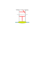
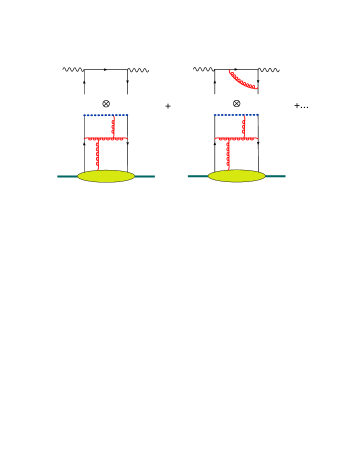
Figure 1: Expansion of the ${\rm T}$ product of two electromagnetic currents in terms of non-local string operators

As already mentioned above, due to the two different scales of transverse momentum $k_{\perp}$, in DIS it is natural to factorize the amplitude of the process in the product of contributions of hard and soft parts coming from the regions of small and large transverse momenta, respectively. Usually one introduces a factorization scale $\mu$ to separate the hard and perturbative part from the soft and not perturbative part. The integrals over $k^{2}_{\perp}>\mu^{2}$ give the coefficient functions in front of light-cone operators while the contributions from $k^{2}_{\perp}<\mu^{2}$ give matrix elements of these operators normalized at the normalization point $\mu$. The evolution of such matrix elements with respect to the renormalization poit $\mu$ is the DGLAP evolution equation. The expansion in terms of string operators is diagrammatically given in Fig. 1 where dotted lines represent the gauge link

$${\rm Pexp}\Big{(}ig\int_{0}^{1}du(x-y)_{\mu}A^{\mu}(xu+(1-u)y)\Big{)}$$ (1)

Let us now turn our discussion to the case of high-energy (Regge) limit where all the transverse momenta are of the same order of magnitude and therefore it is natural to introduce a different factorization scale that is the rapidity. Factorization in rapidity means that at high-energy scattering one introduces a rapidity divide $\eta$ which separate ”fast” field from ”slow” fields. Thus, the amplitude of the process can be represented as a convolution of contributions coming from fields with rapidity $\eta<Y$ ( fast field) and contributions coming from fields with rapidity $\eta>Y$ ( slow fields). As in the case of the usual OPE, the integration over the field with rapidity $\eta<Y$ gives us the coefficients function while the integrations over the field with rapidity $\eta>Y$ are the matrix elements of the operators. A general feature of high-energy scattering is that a fast particle moves along its straight-line classical trajectory and the only quantum effect is the eikonal phase factor acquired along this propagation path. In QCD, for the fast quark or gluon scattering off some target, this eikonal phase factor is a Wilson line - the infinite gauge link ordered along the straight line collinear to particle’s velocity $n^{\mu}$:

$$U^{\eta}(x_{\perp})={\rm Pexp}\Big{\{}ig\int_{-\infty}^{\infty}\!\!du~{}n_{\mu}~{}A^{\mu}(un+x_{\perp})\Big{\}},~{}~{}~{}~{}$$ (2)

Here $A_{\mu}$ is the gluon field of the target, $x_{\perp}$ is the transverse position of the particle which remains unchanged throughout the collision, and the index $\eta$ labels the rapidity of the particle. Repeating the above argument for the target (moving fast in the spectator’s frame) we see that particles with very different rapidity perceive each other as Wilson lines and therefore these Wilson-line operators form the convenient effective degrees of freedom in high-energy QCD (for a review, see Ref. mobzor ). The expansion of the ${\rm T}$ product of two electromagnetic currents at high-energy (Regge limit) is then in terms of Wilson lines

$$T\{\hat{j}_{\mu}(x)\hat{j}_{\nu}(y)\}=\int\!d^{2}z_{1}d^{2}z_{2}~{}I^{\rm LO}_{\mu\nu}(z_{1},z_{2}){\rm Tr}\{\hat{U}^{\eta}_{z_{1}}\hat{U}^{\dagger\eta}_{z_{2}}\}$$

$$+\int\!d^{2}z_{1}d^{2}z_{2}d^{2}z_{3}~{}I^{\rm NLO}_{\mu\nu}(z_{1},z_{2},z_{3})[{\rm tr}\{\hat{U}^{\eta}_{z_{1}}\hat{U}^{\dagger\eta}_{z_{3}}\}{\rm tr}\{\hat{U}^{\eta}_{z_{3}}\hat{U}^{\dagger\eta}_{z_{2}}\}-N_{c}{\rm tr}\{\hat{U}^{\eta}_{z_{1}}\hat{U}^{\dagger\eta}_{z_{2}}\}]$$

We indicate operators by ”hat”. The diagrammatic version of eq. (II) is given in Fig. 2: the dotted lines represent the Wilson lines while the coefficients functions are represented by the propagation of the $q\bar{q}$ pair in the background of shock-wave (represented in the figure by the red strip).

Figure 2: High-energy operator expansion in Wilson lines

In Ref. nlobkN4 such expansion is performed in the ${\cal N}=4$ SYM theory for two BPS-protected currents ${{\cal O}}\equiv{4\pi^{2}\sqrt{2}\over\sqrt{N_{c}^{2}-1}}{\rm Tr\{Z^{2}\}}$ ($Z={1\over\sqrt{2}}(\phi_{1}+i\phi_{2})$) and it is given by

$$(x-y)^{4}T\{\hat{\cal O}(x)\hat{\cal O}(y)\}~{}=~{}{(x-y)^{4}\over\pi^{2}(N_{c}^{2}-1)}\!\int\!d^{2}z_{1\perp}d^{2}z_{2\perp}{(x_{\ast}y_{\ast})^{-2}\over{\cal Z}_{1}^{2}{\cal Z}_{2}^{2}}~{}[{\rm Tr}\{\hat{U}^{\eta}_{z_{1}}\hat{U}^{\dagger\eta}_{z_{2}}\}]^{\rm conf}$$

$$-~{}{\alpha_{s}(x-y)^{4}\over 2\pi^{4}(N_{c}^{2}-1)}\!\int\!d^{2}z_{1\perp}d^{2}z_{2\perp}d^{2}z_{3}{z_{12}^{2}(x_{\ast}y_{\ast})^{-2}\over z_{13}^{2}z_{23}^{2}{\cal Z}_{1}^{2}{\cal Z}_{2}^{2}}\Big{(}\ln{a\sigma^{2}s^{2}z_{12}^{2}\over 16z_{13}^{2}z_{23}^{2}}\Big{[}{(x-z_{3})^{2}\over x_{\ast}}-{(y-z_{3})^{2}\over y_{\ast}}\Big{]}^{2}$$

$$\hskip 11.38109pt-i\pi+2C\Big{)}[{\rm Tr}\{T^{n}\hat{U}^{\eta}_{z_{1}}\hat{U}^{\dagger\eta}_{z_{3}}T^{n}\hat{U}^{\eta}_{z_{3}}\hat{U}^{\dagger\eta}_{z_{2}}\}-N_{c}{\rm Tr}\{\hat{U}^{\eta}_{z_{1}}\hat{U}^{\dagger\eta}_{z_{2}}\}]$$ (3)

where

$$[{\rm Tr}\{\hat{U}^{\eta}_{z_{1}}\hat{U}^{\dagger\eta}_{z_{2}}\}\big{]}^{\rm conf}={\rm Tr}\{\hat{U}^{\eta}_{z_{1}}\hat{U}^{\dagger\eta}_{z_{2}}\}$$

$$+{\alpha_{s}\over 2\pi^{2}}\!\int\!d^{2}z_{3}~{}{z_{12}^{2}\over z_{13}^{2}z_{23}^{2}}[{\rm Tr}\{T^{n}\hat{U}^{\eta}_{z_{1}}\hat{U}^{\dagger\eta}_{z_{3}}T^{n}\hat{U}^{\eta}_{z_{3}}\hat{U}^{\dagger\eta}_{z_{2}}\}-N_{c}{\rm Tr}\{\hat{U}^{\eta}_{z_{1}}\hat{U}^{\dagger\eta}_{z_{2}}\}]\ln{az_{12}^{2}\over z_{13}^{2}z_{23}^{2}}$$ (4)

is the composite dipole with the conformal longitudinal cutoff in the next-to-leading order. The appearance of the composite operators is due to the loss of conformal invariance of the Wilson line operator in the NLO. Indeed, the light-like Wilson lines $U(x_{\perp})$ are formally Möbius invariant and consequently the leading-order BK equation is also conformal invariant. At NLO the Wilson line operator are divergent and its regularization introduces a dependence on the rapidity and conformal symmetry is lost. In order to restore the conformal invariance we redefine the operator ${\rm Tr}\{\hat{U}^{\eta}_{z_{1}}\hat{U}^{\dagger\eta}_{z_{2}}\}$ by adding suitable conterterms. This procedure of finding the dipole with conformally regularized rapidity divergence is analogous to the construction of the composite renormalized local operator by adding the appropriate counterterms order by order in perturbation theory.

III Leading order evolution of color dipoles

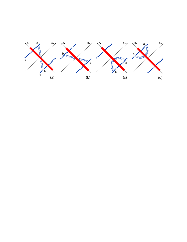
Figure 3: Leading-order diagrams for the small-$x$ evolution of color dipole. Wilson lines are denoted by dotted lines.

Let us consider now the deep inelastic scattering from a hadron at small $x_{B}$. As previously explained, the virtual photon decomposes into a pair of fast quarks moving along straight lines separated by some transverse distance. The propagation of this quark-antiquark pair reduces to the “propagator of the color dipole” that is two Wilson lines ordered along the direction collinear to quarks’ velocity: $U(x_{\perp})U^{\dagger}(y_{\perp})$. The structure function of a hadron is proportional to a matrix element of this color dipole operator

$$\hat{\cal U}^{\eta}(x_{\perp},y_{\perp})=1-{1\over N_{c}}{\rm Tr}\{\hat{U}^{\eta}(x_{\perp})\hat{U}^{\dagger\eta}(y_{\perp})\}$$ (5)

switched between the target’s states ($N_{c}=3$ for QCD). The gluon parton density is approximately

$$x_{B}G(x_{B},\mu^{2}=Q^{2})~{}\simeq~{}\left.\langle p|~{}\hat{\cal U}^{\eta}(x_{\perp},0)|p\rangle\right|_{x_{\perp}^{2}=Q^{-2}}$$ (6)

where $\eta=\ln{1\over x_{B}}$. The energy dependence of the structure function is translated then into the dependence of the color dipole on the slope of the Wilson lines determined by the rapidity $\eta$. Thus, the small-x behavior of the structure functions is governed by the rapidity evolution of color dipolesdipole . At relatively high energies and for sufficiently small dipoles we can use the leading logarithmic approximation (LLA) where $\alpha_{s}\ll 1$, $\alpha_{s}\ln x_{B}\sim 1$ and get the non-linear BK evolution equation for the color dipolesba96 ; yura :

$${d\over d\eta}~{}\hat{\cal U}(x,y)={\alpha_{s}N_{c}\over 2\pi^{2}}\!\int\!d^{2}z~{}{(x-y)^{2}\over(x-z)^{2}(z-y)^{2}}[\hat{\cal U}(x,z)+\hat{\cal U}(y,z)$$

$$\hskip 142.26378pt-\hat{\cal U}(x,y)-\hat{\cal U}(x,z)\hat{\cal U}(z,y)]$$ (7)

The first three terms correspond to the linear BFKL evolutionbfkl and describe the parton emission while the last term is responsible for the parton annihilation. For sufficiently high $x_{B}$ the parton emission balances the parton annihilation so the partons reach the state of saturation saturation with the characteristic transverse momentum $Q_{s}$ growing with energy $1/x_{B}$.

IV NLO evolution of color dipole

The NLO evolution of color dipole in QCD performed in Ref. nlobk is not expected to be Möbius invariant due to the conformal anomaly leading to dimensional transmutation and running coupling constant. However, the NLO BK equation in QCD has an additional term violating Möbius invariance and not related to the conformal anomaly. To understand the relation between the high-energy behavior of amplitudes and Möbius invariance of Wilson lines, it is instructive to consider the conformally invariant ${\cal N}=4$ super Yang-Mils theory. This theory was intensively studied in recent years due to the fact that at large coupling constants it is dual to the IIB string theory in the AdS₅ background. In the light-cone limit, the contribution of scalar operators to Maldacena-Wilson linemwline vanishes so one has the usual Wilson line constructed from gauge fields and therefore the LLA evolution equation for color dipoles in the ${\cal N}=4$ SYM has the same form as (7). At the NLO level, the contributions from gluino and scalar loops enter the picture. As we mentioned above, formally the light-like Wilson lines are Möbius invariant. We also mentioned that the light-like Wilson lines are divergent in the longitudinal direction and moreover, it is exactly the evolution equation with respect to this longitudinal cutoff which governs the high-energy behavior of amplitudes. At present, it is not known how to find the conformally invariant cutoff in the longitudinal direction. When we use the non-invariant cutoff we expect, as usual, the invariance to hold in the leading order but to be violated in higher orders in perturbation theory. In the calculation of Ref. nlobkN4 we restrict the longitudinal momentum of the gluons composing Wilson lines, and with this non-invariant cutoff the NLO evolution equation in QCD has extra non-conformal parts not related to the running of coupling constant. Similarly, there will be non-conformal parts coming from the longitudinal cutoff of Wilson lines in the ${\cal N}=4$ SYM equation. Here we present the result for the NLO evolution of the color dipole in ${\cal N}=4$ SYM ( performed in Ref. nlobkN4 ) in the adjoint representation (we use notations $z_{ij}\equiv z_{i}-z_{j}$ and $(T^{a})_{bc}=-if^{abc}$)

$${d\over d\eta}\big{[}{\rm Tr}\{\hat{U}^{\eta}_{z_{1}}\hat{U}^{\dagger\eta}_{z_{2}}\}\big{]}^{\rm conf}~{}$$ (8)

$$={\alpha_{s}\over\pi^{2}}\!\int\!d^{2}z_{3}~{}{z_{12}^{2}\over z_{13}^{2}z_{23}^{2}}\Big{[}1-{\alpha_{s}N_{c}\over 4\pi}{\pi^{2}\over 3}\Big{]}\big{[}{\rm Tr}\{T^{a}\hat{U}^{\eta}_{z_{1}}\hat{U}^{\dagger\eta}_{z_{3}}T^{a}\hat{U}_{z_{3}}\hat{U}^{\dagger\eta}_{z_{2}}\}-N_{c}{\rm Tr}\{\hat{U}^{\eta}_{z_{1}}\hat{U}^{\dagger\eta}_{z_{2}}\}\big{]}^{\rm conf}$$

$$-{\alpha_{s}^{2}\over 4\pi^{4}}\int\!d^{2}z_{3}d^{2}z_{4}{z_{12}^{2}\over z_{13}^{2}z_{24}^{2}z_{34}^{2}}\Big{\{}2\ln{z_{12}^{2}z_{34}^{2}\over z_{14}^{2}z_{23}^{2}}+\Big{[}1+{z_{12}^{2}z_{34}^{2}\over z_{13}^{2}z_{24}^{2}-z_{14}^{2}z_{23}^{2}}\Big{]}\ln{z_{13}^{2}z_{24}^{2}\over z_{14}^{2}z_{23}^{2}}\Big{\}}$$

$$\times{\rm Tr}\{[T^{a},T^{b}]\hat{U}^{\eta}_{z_{1}}T^{a^{\prime}}T^{b^{\prime}}\hat{U}^{\dagger\eta}_{z_{2}}+T^{b}T^{a}\hat{U}^{\eta}_{z_{1}}[T^{b^{\prime}},T^{a^{\prime}}]\hat{U}^{\dagger\eta}_{z_{2}}\}[(\hat{U}^{\eta}_{z_{3}})^{aa^{\prime}}(\hat{U}^{\eta}_{z_{4}})^{bb^{\prime}}-(z_{4}\rightarrow z_{3})]$$

where $a$ is an arbitrary dimensional constant. In fact, $a(\eta)=ae^{\eta}$ plays the same role for the rapidity evolution as $\mu^{2}$ for the usual DGLAP evolution: the derivative ${d\over da}$ gives the evolution equation (8). The kernel in the r.h.s. of Eq. (8) is obviously Möbius invariant since it depends on two four-point conformal ratios ${z_{13}^{2}z_{24}^{2}\over z_{14}^{2}z_{23}^{2}}$ and ${z_{12}^{2}z_{34}^{2}\over z_{13}^{2}z_{24}^{2}}$. In nlobkN4 we also demonstrate that Eq. (8) agrees with forward NLO BFKL calculation of Ref. lipkot . Let us now present the calculation for the NLO BK kernel in the case of QCD

$${d\over d\eta}\big{[}{\rm tr}\{\hat{U}^{\eta}_{z_{1}}\hat{U}^{\dagger\eta}_{z_{2}}\}\big{]}^{\rm conf}~{}=~{}{\alpha_{s}\over 2\pi^{2}}\!\int\!d^{2}z_{3}~{}{z_{12}^{2}\over z_{13}^{2}z_{23}^{2}}\Big{[}1$$

$$+~{}{\alpha_{s}\over 4\pi}\Big{[}b(\ln{z_{12}^{2}\mu^{2}\over 4}+2C)-b{z_{13}^{2}-z_{23}^{2}\over z_{12}^{2}}\ln{z_{13}^{2}\over z_{23}^{2}}+\big{(}{67\over 9}-{\pi^{2}\over 3}\big{)}N_{c}-{10\over 9}n_{f}\Big{]}$$

$$\times\big{[}{\rm tr}\{\hat{U}^{\eta}_{z_{1}}\hat{U}^{\dagger\eta}_{z_{3}}\}{\rm tr}\{\hat{U}^{\eta}_{z_{3}}\hat{U}^{\dagger\eta}_{z_{2}}\}-N_{c}{\rm tr}\{\hat{U}^{\eta}_{z_{1}}\hat{U}^{\dagger\eta}_{z_{2}}\}\big{]}^{\rm conf}$$

$$+~{}{\alpha_{s}^{2}\over 16\pi^{4}}\int\!{d^{2}z_{3}d^{2}z_{4}\over z_{34}^{4}}\Bigg{[}\Big{\{}\Big{(}-2+2{z_{12}^{2}z_{34}^{2}\over z_{13}^{2}z_{24}^{2}}\ln{z_{12}^{2}z_{34}^{2}\over z_{14}^{2}z_{23}^{2}}$$

$$+\Big{[}{z_{12}^{2}z_{34}^{2}\over z_{13}^{2}z_{24}^{2}}\big{(}1+{z_{12}^{2}z_{34}^{2}\over z_{13}^{2}z_{24}^{2}-z_{14}^{2}z_{23}^{2}}\big{)}+{2z_{13}^{2}z_{24}^{2}-4z_{12}^{2}z_{34}^{2}\over z_{13}^{2}z_{24}^{2}-z_{14}^{2}z_{23}^{2}}\Big{]}\ln{z_{13}^{2}z_{24}^{2}\over z_{14}^{2}z_{23}^{2}}\Big{)}+~{}\big{(}z_{3}\leftrightarrow z_{4}\big{)}\Big{\}}$$

$$\times~{}\big{[}\big{(}{\rm tr}\{\hat{U}^{\eta}_{z_{1}}\hat{U}^{\dagger\eta}_{z_{3}}\}{\rm tr}\{\hat{U}^{\eta}_{z_{3}}\hat{U}^{\dagger\eta}_{z_{4}}\}{\rm tr}\{\hat{U}^{\eta}_{z_{4}}\hat{U}^{\dagger\eta}_{z_{2}}\}-{\rm tr}\{\hat{U}^{\eta}_{z_{1}}\hat{U}^{\dagger\eta}_{z_{3}}\hat{U}^{\eta}_{z_{4}}\hat{U}^{\dagger\eta}_{z_{2}}\hat{U}^{\eta}_{z_{3}}\hat{U}^{\dagger\eta}_{z_{4}}\}\big{)}-(z_{4}\rightarrow z_{3})\big{]}$$

$$+~{}{z_{12}^{2}z_{34}^{2}\over z_{13}^{2}z_{24}^{2}}\Big{\{}2\ln{z_{12}^{2}z_{34}^{2}\over z_{14}^{2}z_{23}^{2}}+\Big{[}1+{z_{12}^{2}z_{34}^{2}\over z_{13}^{2}z_{24}^{2}-z_{14}^{2}z_{23}^{2}}\Big{]}\ln{z_{13}^{2}z_{24}^{2}\over z_{14}^{2}z_{23}^{2}}\Big{\}}$$

$$\times\big{(}{\rm tr}\{\hat{U}^{\eta}_{z_{1}}\hat{U}^{\dagger\eta}_{z_{3}}\}{\rm tr}\{\hat{U}^{\eta}_{z_{3}}\hat{U}^{\dagger\eta}_{z_{4}}\}{\rm tr}\{\hat{U}^{\eta}_{z_{4}}\hat{U}^{\dagger\eta}_{z_{2}}\}-z_{3}\leftrightarrow z_{4}\big{)}\Bigg{]}$$

$$+~{}{\alpha^{2}_{s}n_{f}\over 2\pi^{4}}\!\int\!{d^{2}z_{3}d^{2}z_{4}\over z_{34}^{4}}\Big{\{}2-{z_{13}^{2}z_{24}^{2}+z_{23}^{2}z_{14}^{2}-z_{12}^{2}z_{34}^{2}\over z_{13}^{2}z_{24}^{2}-z_{14}^{2}z_{23}^{2}}\ln{z_{13}^{2}z_{24}^{2}\over z_{14}^{2}z_{23}^{2}}\Big{\}}$$

$$\times{\rm tr}\{t^{a}\hat{U}^{\eta}_{z_{1}}t^{b}\hat{U}^{\dagger\eta}_{z_{2}}\}{\rm tr}\{t^{a}\hat{U}^{\eta}_{z_{3}}t^{b}(\hat{U}^{\dagger\eta}_{z_{4}}-\hat{U}^{\eta}_{z_{3}})\}$$

(9)

where $b={11\over 3}N_{c}-{2\over 3}n_{f}$. As previously advertised the NLO BK kernel in QCD for the composite operators resolves in a sum of the conformal part and the running-coupling part.

V Conclusions

We have discussed the DIS scattering in the Bjorken Limit and in the Regge limit; we have briefly reviewed the standard techniques used to study DIS, that is OPE in local operators and in non-local string operator. This allowed us to introduce the OPE at high-energy of the ${\rm T}$ of two electromagnetic current in terms of Wilson lines operators. We have observed the BFKL equation gives us a nice prediction of the increase of the parton density at high energy, but it fails at very high energy since it would violate the unitarity condition. The recombination phenomena of partons occurring at very high energies are governed by non-linear effects (coherency effects) which can be taken into account only by a non-linear equation. Furthermore, we have seen that in order to recover the unitarization of the theory, the system eventually evolves towards a saturation region. Then Breit frame introduced above is not anymore a suitable frame to describe DIS processes. Instead, we considered the so called dipole frame which is a natural frame work for the description of multiple scattering which are relevant at high energy. The evolution of Wilson line operator ${\cal U}(x_{\perp},y_{\perp})$ is the needed non linear equation for the description of the coherency effect appearing at this regime. This evolution equation is the BK equation. At the end we have presented the result for the NLO kernel of the BK equation in the case of QCD and in the ${N}=4$ SYM theory. In order to restore conformal symmetry we have introduced the conformal composite operator.

References

- (1) V.N. Gribov and L.N. Lipatov, Sov. Journ. Nucl. Phys. 15 438 (1972); G. Altarelli and G. Parisi, Nucl. Phys. B126 298 (1977); Yu. L. Dokshitzer, Sov. Phys. JETP 46 641 (1977).
- (2) C. Adloff et al. [H1 Collaboration], Eur. Phys. J. C 21 (2001) 33 [arXiv:hep-ex/0012053]; S. Chekanov et al. [ZEUS Collaboration], Eur. Phys. J. C 21 (2001) 443 [arXiv:hep-ex/0105090].
- (3) V.S. Fadin, E.A. Kuraev, and L.N. Lipatov, Phys. Lett. B 60, (1975) 50; I. Balitsky and L.N. Lipatov, Sov. Journ. Nucl. Phys. 28, (1978) 822.
- (4) L.V. Gribov, E.M. Levin, and M.G. Ryskin, Phys. Rept. 100, 1 (1983), A.H. Mueller and J.W. Qiu, Nucl. Phys. B268, 427 (1986); A.H. Mueller, Nucl. Phys. B335, 115 (1990).
- (5) I. Balitsky, Nucl. Phys. B463, 99 (1996); “Operator expansion for diffractive high-energy scattering”, [hep-ph/9706411];
- (6) Yu.V. Kovchegov, Phys. Rev. D60, 034008 (1999); Phys. Rev. D61,074018 (2000).
- (7) K. G. Wilson, Phys. Rev. 179, 1499 (1969).
- (8) I. I. Balitsky, Phys. Lett. B 124, 230 (1983).
- (9) A. V. Efremov and A. V. Radyushkin, Phys. Lett. B 94, 245 (1980). G. P. Lepage and S. J. Brodsky, Phys. Rev. D 22 (1980) 2157. M. K. Chase, Nucl. Phys. B 174, 109 (1980). T. Ohrndorf, Nucl. Phys. B 186, 153 (1981).
- (10) I. I. Balitsky and V. M. Braun, Nucl. Phys. B 311, 541 (1989).
- (11) I. Balitsky, “High-Energy QCD and Wilson Lines”, In *Shifman, M. (ed.): At the frontier of particle physics, vol. 2*, p. 1237-1342 (World Scientific, Singapore,2001) [hep-ph/0101042]
- (12) I. Balitsky and G. A. Chirilli, Nucl. Phys. B 822 (2009) 45 [arXiv:0903.5326 [hep-ph]].
- (13) A.H. Mueller, Nucl. Phys. B415, 373 (1994); A.H. Mueller and Bimal Patel, Nucl. Phys. B425, 471 (1994). N.N. Nikolaev and B.G. Zakharov, Phys. Lett. B 332, 184 (1994); Z. Phys. C64, 631 (1994); N.N. Nikolaev B.G. Zakharov, and V.R. Zoller, JETP Letters 59, 6 (1994).
- (14) I. Balitsky and G. A. Chirilli, Phys. Rev. D 77 (2008) 014019 [arXiv:0710.4330 [hep-ph]].
- (15) J.M. Maldacena, Phys.Rev.Lett. 80, 4859 (1998).
- (16) A.V. Kotikov and L.N. Lipatov, Nucl. Phys. B582, 19 (2000); Nucl. Phys. B5661, 19 (2003). Erratum-ibid., B685, 405 (2004).