Soliton absorption spectroscopy

Abstract

We analyze optical soliton propagation in the presence of weak absorption lines with much narrower linewidths as compared to the soliton spectrum width using the novel perturbation analysis technique based on an integral representation in the spectral domain. The stable soliton acquires spectral modulation that follows the associated index of refraction of the absorber. The model can be applied to ordinary soliton propagation and to an absorber inside a passively modelocked laser. In the latter case, a comparison with water vapor absorption in a femtosecond Cr:ZnSe laser yields a very good agreement with experiment. Compared to the conventional absorption measurement in a cell of the same length, the signal is increased by an order of magnitude. The obtained analytical expressions allow further improving of the sensitivity and spectroscopic accuracy making the soliton absorption spectroscopy a promising novel measurement technique.

I introduction

Light sources based on femtosecond pulse oscillators have now become widely used tools for ultrashort studies, optical metrology, and spectroscopy. Such sources combine broad smooth spectra with diffraction-limited brightness, which is especially important for high-sensitivity spectroscopic applications. Advances in near- and mid-infrared femtosecond oscillators made possible operation in the wavelength ranges of strong molecular absorption, allowing direct measurement of important molecular gases with high resolution and good signal-to-noise ratio extra . At the same time, it was observed that such oscillators behave quite differently, when the absorbing gas fills the laser cavity or introduced after the output mirror EP-exp ; EP-theor . The issue has become especially important with introduction of the mid-IR femtosecond oscillators such as Cr:ZnSe CZS-1 , which operate in the 2–3 $\mu$m wavelength region with strong atmospheric absorption.

As an example, Figure 1 presents a typical spectrum of a Cr:ZnSe femtosecond oscillator, operating at normal atmospheric conditions. It is clearly seen, that the pulse spectrum acquires strong modulation features which resemble the dispersion signatures of the atmospheric lines. Being undesirable for some applications, such spectral modulation might at the same time open up interesting opportunity of intracavity absorption spectroscopy. Compared with the traditional intracavity laser absorption spectroscopy ICLAS-gen ; ICLAS-CZS based on transient processes, this approach would have an advantage of being a well-quantified steady-state technique, that can be immediately coupled to frequency combs and optical frequency standards for extreme accuracy and resolution.

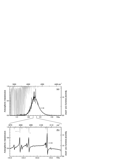
Figure 1: Output spectrum of a 100-fs Cr:ZnSe oscillator (black solid line) when operated at open air. The atmospheric transmission (gray) is calculated from HITRAN database HITRAN and corresponds to a full round-trip. The lower graph (b) shows the expanded central part of the spectrum. Asterisk denotes the absorption line, which is used for quantitative evaluation in the last section.

In this paper, we present a numerical and analytical treatment of the effect of a narrowband absorption on a femtosecond pulse, considered as a dissipative soliton. Such a treatment covers both, passively modelocked ultrashort pulse oscillators with intracavity absorbers, and soliton propagation in fibers with impurities. The theoretical results are compared with the experiment for a femtosecond Cr:ZnSe oscillator operating at normal atmospheric conditions. We prove that the spectral modulation imposed by a narrowband absorption indeed accurately follows the associated index of refraction when the absorber linewidth is sufficiently narrow.

II The model

Our approach is based on the treatment of an ultrashort pulse as one-dimensional dissipative soliton of the nonlinear complex Ginzburg-Landau equation (CGLE) Haus-apm ; nail . This equation has such a wide horizon of application that the concept of “the world of the Ginzburg-Landau equation” has become broadly established kramer . In particular, such a model describes a pulse with the duration $T_{0}$ inside an oscillator or propagating along a nonlinear fiber.

To obey the CGLE, the electromagnetic field with the amplitude $A(z,t)$ should satisfy the slowly-varying amplitude approximation, provided by the relation $\omega_{0}\gg 1/T_{0}$, where $\omega_{0}$ is the field carrier frequency, $t$ is the local time, and $z$ is the propagation coordinate. This approximation is well satisfied even for pulses of nearly single optical cycle duration TB-FK . When additionally we can neglect the field variation along the cavity round-trip or the variation of material parameters along a fiber, as well as the contribution of higher-order dispersions, the amplitude dynamics can be described on the basis of the generalized CGLE nail ; kaertner ; nail-2 ; akhmanov

$$\frac{\partial A(z,t)}{\partial z}=\left\{-\sigma+\hat{\Sigma}[P(z,t)]-i\gamma P(z,t)\right\}A(z,t)+\left(\alpha+i\frac{\beta_{2}}{2}\right)\frac{\partial^{2}}{\partial t^{2}}A(z,t)+\hat{\Gamma}\left[A(z,t)\right],$$ (1)

where $P\equiv\left|A\right|^{2}$ is the instant field power and $\alpha$ is the inverse gain bandwidth squared. The nonlinear terms in Eq. (1) describe i) saturable self-amplitude modulation (SAM) with nonlinear gain defined by the nonlinear operator $\hat{\Sigma}$, and ii) self-phase modulation (SPM), defined by the parameter $\gamma$. For a laser oscillator, $\gamma=4\pi nn_{2}l_{cryst}/\lambda_{0}A_{eff}$. Here $\lambda_{0}$ is the wavelength; $n$ and $n_{2}$ are the linear and nonlinear refractive indexes of an active medium, respectively; $l_{cryst}$ is the length of the active medium; $A_{eff}=\pi w^{2}$ is the effective area of a Gaussian mode with the radius $w$ inside the active medium. The propagation coordinate $z$ is naturally normalized to the cavity length, i.e. $z$ becomes the cavity round-trip number. For a fiber propagation, $\gamma=2\pi nn_{2}/\lambda_{0}A_{eff}$, where $n$ and $n_{2}$ are the linear and nonlinear refractive indexes of a fiber, respectively, and $A_{eff}$ is the effective mode area of the fiber agrawal . Finally, $\beta_{2}$ is the round-trip net group delay dispersion (GDD) for an oscillator or the group velocity dispersion parameter for a fiber with $\beta_{2}<0$ corresponding to anomalous dispersion.

The typical explicit expressions for $\hat{\Sigma}[P]$ in the case, when the SAM response is instantaneous, are i) $\hat{\Sigma}[P]=\kappa P$ (cubic nonlinear gain), ii) $\hat{\Sigma}[P]=\kappa\left(P-\zeta P^{2}\right)$ (cubic-quintic nonlinear gain), and iii) $\hat{\Sigma}[P]=\kappa P/\left(1+\zeta P\right)$ (perfectly saturable nonlinear gain) nail ; nonkerr . The second case corresponds to an oscillator mode-locked by the Kerr-lensing Haus-apm . The third case represents, for instance, a response of a semiconductor saturable absorber, when $T_{0}$ exceeds its excitation relaxation time sesam . However, if the latter condition is not satisfied, one has to add an ordinary differential equation for the SAM and Eq. (1) becomes an integro-differential equation (see below).

The $\sigma$-term is the saturated net-loss at the carrier frequency $\omega_{0}$, which is the reference frequency in the model. This term is energy-dependent: the pulse energy $E(z)\equiv\intop_{-\infty}^{\infty}P(z,t)dt$ can be expanded in the vicinity of threshold value $\sigma=0$ as $\sigma\approx\delta\left(E/E^{*}-1\right)$ apb , where $\delta=\ell^{2}/g_{0}$ ($\ell$ is the frequency-independent loss and $g_{0}$ is the small-signal gain, both for the round-trip) and $E^{*}$ is the round-trip continuous-wave energy equal to the average power multiplied by the cavity period.

The operator $\hat{\Gamma}$ describes an effect of the frequency-dependent losses, which can be attributed to an absorption within the dissipative soliton spectrum. That can be caused, for instance, by the gases filling an oscillator cavity or the fiber impurities for a fiber oscillator. Within the framework of this study, we neglect the effects of loss saturation and let $\hat{\Gamma}$ be linear with respect to $A\left(z,t\right)$. The expression for $\hat{\Gamma}\left[A(z,t)\right]$ is more convenient to describe in the Fourier domain, $\tilde{A}(z,\omega)$ being the Fourier image of $A(z,t)$. If the losses result from the $l$ independent homogeneously broadened lines centered at $\omega_{l}$ (relative to $\omega_{0}$) with linewidths $\Omega_{l}$ and absorption coefficients $\epsilon_{l}<0$, then the action of operator $\hat{\Gamma}$ can be written down in the form of a superposition of causal Lorentz profiles butilkin ; lorentz

$$\hat{\Gamma}\left[\tilde{A}\right]=\left(\sum_{l}\frac{\epsilon_{l}}{1+i(\omega-\omega_{l})/\Omega_{l}}\right)\tilde{A}(z,\omega).$$ (2)

In the more general case the causal Voigt profile has to be used for $\hat{\Gamma}\left[\tilde{A}\right]$ cVoigt . Causality of the complex profile of Eq. (2) demonstrates itself in the time domain, where one has

$$\hat{\Gamma}\left[A\left(z,t\right)\right]\propto\sum_{l}\epsilon_{l}\Omega_{l}\intop_{-\infty}^{t}e^{-\left(\Omega_{l}-i\omega_{l}\right)\left(t-t^{\prime}\right)}A\left(z,t^{\prime}\right)dt^{\prime}.$$ (3)

The conventional analysis of perturbed soliton propagation includes approximation of the effective group delay dispersion of the perturbation as Taylor series $\beta^{\prime}(\omega)=\beta_{2}^{\prime}(\omega-\omega_{0})^{2}/2+\beta_{3}^{\prime}(\omega-\omega_{0})^{3}/6,\dots$ assuming that the additional terms $\beta_{2}^{\prime},\beta_{3}^{\prime},\dots$ are sufficiently small. This approach is absolutely not applicable in our case, because the dispersion, associated with a narrow linewidth absorber can be extremely large. For example, an atmospheric line with a typical width $\Omega=3$GHz and peak absorption of only $10^{-3}$ produces the group delay dispersion modulation of $\beta_{2}^{\prime}=\pm 0.9$ ns², far exceeding the typical intracavity values of $\beta_{2}\sim 10^{2}..10^{4}$ fs². Moreover, decreasing the linewidth $\Omega$ (and thus reducing the overall absorption of the line) causes the group delay dispersion term to diverge as $\beta_{2}^{\prime}\propto\Omega^{-2}$.

In the following we shall therefore start with a numerical analysis to establish the applicability and stability of the model, and then present a novel analysis technique based on integral representation in the spectral domain.

III Numerical analysis

Without introducing any additional assumptions, we have solved the Eqs. (1,2) numerically by the symmetrized split-step Fourier method. To provide high spectral resolution, the simulation local time window contains $2^{22}$ points with the mesh interval 2.5 fs. The simulation parameters for the cubic-quintic version of Eq. (1) are presented in Table 1. The GDD parameter $\beta_{2}=-$1600 fs² provides a stable single pulse with FWHM $\approx$100 fs. The single low-power seeding pulse converges to a steady-state solution during $z\approx$5000.

$E^{*}$	$\gamma$	$\alpha$	$\kappa$	$\zeta$	$\delta$	$\beta_{2}$
20 nJ	2.5 MW-1	16 fs2	0.02$\gamma$	0.2$\gamma$	0.03	-1600 fs2

Table 1: Laser simulation parameters. The numbers correspond to a Cr:ZnSe femtosecond oscillator of Fig. 1 with $l_{cryst}=$0.4 cm, $w=$80 $\mu$m, $\lambda_{0}=$2.5 $\mu$m, $n=2.44$, $n_{2}=10^{-14}$ cm${}^{2}/$W, $\ell=$0.075, $g_{0}=$2.5$\ell$.

The pulse propagation within a linear medium (e.g. an absorbing gas outside an oscillator, a passive fiber containing some impurities, or microstructured fiber filled with a gas) is described by Eqs. (1,2) with zero $\alpha$, $\gamma$, $\hat{\Sigma}$, and the initial $A\left(0,t\right)$ corresponding to output oscillator pulse. The obvious effect of the absorption lines on a pulse spectrum are the dips at $\omega_{l}$ (Fig. 4a), that simply follow the Beer’s law. This regime allows using the ultrashort pulse for conventional absorption spectroscopy extra . The nonzero real part of an absorber permittivity (i.e. $\Im\left(\hat{\Gamma}\right)\neq$0) does significantly change the pulse in time domain JapsLin , but does not alter the spectrum. The pulse spectrum reveals only imaginary part of an absorber permittivity (i.e. $\Re\left(\hat{\Gamma}\right)\neq$0).

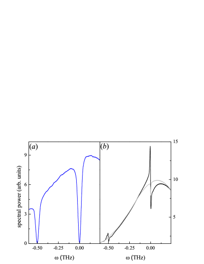
Figure 2: (Color online) Part of the pulse spectrum after: (a) linear propagation for 25 dispersion lengths inside a fiber with two absorption lines and (b) perturbed soliton propagation for 100 dispersion lengths. Gray curve in (b) corresponds to the contribution of only $\Re(\hat{\Gamma})$ in Eq. (2), black curve corresponds to the contribution of the complex profile (2). $\epsilon_{1}=\epsilon_{2}=-0.1$, $\Omega_{1}=\Omega_{2}=40$ GHz. The initial pulse profile is $A\left(t\right)=A_{0}\mathrm{sech}\left(t/T_{0}\right)$, where $T_{0}=$57 fs.

Introducing the nonzero SPM coefficient $\gamma=|\beta_{2}|/A_{0}^{2}T_{0}^{2}$ with zero $\alpha$ and $\hat{\Sigma}$ transforms Eq. (1) to a perturbed nonlinear Schrödinger equation and results in the true perturbed soliton propagation. In this case, as shown in Fig. 2b, the situation becomes dramatically different. Besides the dips in the spectrum shown by the gray curve corresponding to a contribution of $\Re(\hat{\Gamma})$ only, there is a pronounced contribution from the phase change induced by the dispersion of absorption lines (solid curve in Fig. 2b corresponds to the complex profile of $\hat{\Gamma}$ in Eq. (2)). As a result, the spectral profile has the sharp bends with the maximum on the low-frequency side and the minimum on the high-frequency side of the corresponding absorption line. At the same time, the dips in the spectrum due to absorption are strongly suppressed. In addition to spectral features, the soliton decays, acquires a slight shift towards the higher frequencies, and its spectrum gets narrower due to the energy loss.

The soliton spectrum reveals in this case the real part of the absorber permittivity. However, the continuous change of the soliton shape due to energy decay renders the problem as a non-steady state case. The situation becomes different in a laser oscillator, where pumping provides a constant energy flow to compensate the absorption loss.

Let us consider the steady-state intra-cavity narrowband absorption inside a passively modelocked femtosecond oscillator, where the pulse is controlled by the SPM and the SAM, which is described by the cubic-quintic $\hat{\Sigma}$ in Eq. (1) modeling the Kerr-lens mode-locking mechanism kaertner . Such an oscillator can operate both, in the negative dispersion regime kaertner with an chirped-free soliton-like pulse, and in the positive dispersion regime apb , where the propagating pulse acquires strong positive chirp. In this study, we consider only the negative dispersion regime, the positive dispersion regime will be a subject of following studies.

The results of the simulation are shown in Figs. 3 and 4, and they demonstrate the same dispersion-like modulation of the pulse spectrum. Fig. 3 demonstrates action by three narrow ($\Omega=$2 GHz) absorption lines centered at -10, 0 and 10 GHz in the neighborhood of $\omega=0$. One can see (Fig. 3a), that the absorption lines do not cause spectral dips at $\omega_{l}$, but produce sharp bends, very much like the case of the true perturbed Schrödinger soliton considered before. One can also clearly see the collective redistribution of spectral power from higher- to lower-frequencies, which enhances local spectral asymmetry (Fig. 3a). Such an asymmetry suggests that the dominating contribution to a soliton perturbation results from the real part of an absorber permittivity, which, in particular, causes the time-asymmetry of perturbation in the time domain. This asymmetry is seen in time domain as a ns-long modulated exponential precursor in Fig. 3b.

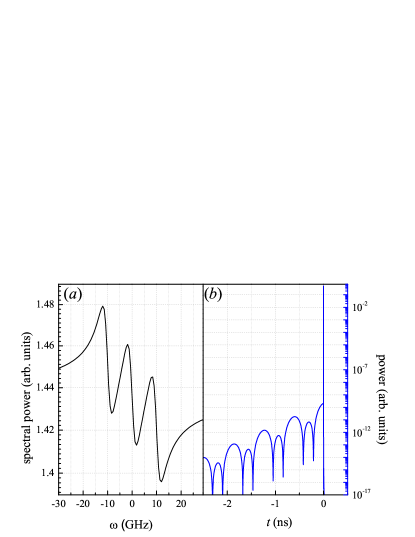
Figure 3: (Color online) Dissipative soliton in an oscillator: (a) central part of the spectrum and (b) power $P(t)$. An oscillator is filled with an absorber described by Eq. (2) with the triplet of lines: $\epsilon_{1}=\epsilon_{2}=\epsilon_{3}=-0.005$, $\Omega_{1}=\Omega_{2}=\Omega_{3}=2$ GHz, and $\omega_{1}=-10$, $\omega_{2}=0$, $\omega_{3}=10$ GHz.

The simulated effect of a single narrow absorption line centered at $\omega=0$ is shown in Fig. 4 for different values of peak absorption $\epsilon$ and width $\Omega$. In Fig. 4a, $\epsilon=-0.05$ and $\Omega=$ 4 GHz (solid curve, open circles and crosses) and 1 GHz (dashed curve, open squares and triangles). The solid and dashed curves demonstrate the action of complex profile (2), whereas circles (squares) and crosses (triangles) demonstrate the separate action of $\Im(\hat{\Gamma})$ and $\Re(\hat{\Gamma})$, respectively. One can see, that the profile of perturbed spectrum traces that formed by only $\Im(\hat{\Gamma})$ (i.e. it traces the real part of an absorber permittivity). One can say, that the pure phase effect ($\Im(\hat{\Gamma})$, circles and squares in Figs. 4a,b) strongly dominates over the pure absorption ($\Re(\hat{\Gamma})$, crosses in Figs. 4a,b), like that for the Schrödinger soliton. Such a domination enhances with a lowered $\epsilon$ (Fig. 4b, crosses), however the $\left|\epsilon\right|$ growth increases the relative contribution of $\Re(\hat{\Gamma})$ and causes the frequency downshift of the bend (Fig. 4a). Amplitude of the bend traces the $\epsilon$ value, while its width is defined by $\Omega$.

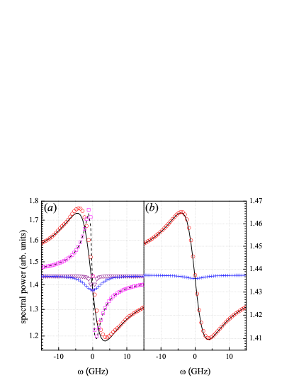
Figure 4: (Color online) Central parts of the dissipative soliton spectra in an oscillator with the single absorption line centered at $\omega=$0. (a) $\epsilon=-0.05$; $\Omega=4$ GHz (solid curve, open circles and crosses) and 1 GHz (dashed curve, open squares and triangles). (b) $\epsilon=-0.005$; $\Omega=4$ GHz. The solid and dashed curves correspond to the contribution of $\hat{\Gamma}$ described by Eq. (2). Open circles and squares describe the separate contribution of $\Im\left(\hat{\Gamma}\right)$. Crosses and triangles describe the separate contribution of $\Re\left(\hat{\Gamma}\right)$.

The SAM considered above is modeled by the cubic-quintic nonlinear term $\hat{\Sigma}$ in Eq.(1). Such a SAM is typically realized by using the self-focusing inside an active medium (Kerr-lens modelocking). For reliable self-starting operation of mode-locked oscillator it is often desirable to use a suitable saturable absorber (SA), e.g. a semiconductor-based SESAM Islam ; keller . Such an absorber can be described in the simplest case by a single-lifetime two-level model, giving the time-dependent loss coefficient $\Lambda\left(t\right)$ as

$$\frac{\partial\Lambda\left(t\right)}{\partial t}=\frac{\Lambda_{0}-\Lambda\left(t\right)}{T_{s}}-\Lambda\left(t\right)\frac{P\left(t\right)}{J_{s}A_{eff}},$$ (4)

where $\Lambda_{0}$ is the loss coefficient for a small signal, $A_{eff}$ is the effective beam area on the SA, $T_{s}$ and $J_{s}$ are the SA relaxation time and the saturation energy fluency, respectively. Eq. (4) supplements Eq. (1) and the SAM term $\hat{\Sigma}$ in the latter has to be replaced by $\left(\Lambda_{0}-\Lambda\left(t\right)\right)$. When the pulse width is longer than the SA relaxation time, one can replace Eq. (4) by its adiabatic solution so that

$$\hat{\Sigma}=\dfrac{\eta_{0}\xi P\left(t\right)}{1+\xi P\left(t\right)},$$ (5)

where $\xi\equiv T_{s}/J_{s}S$ is the inverse saturation power.

We have simulated Eqs. (1,2,4) in the case of $J_{s}=$$50$ $\mu$ J/cm² and $T_{s}=$0.5 ps, that correspond to the measurement in Fig. 1. Two cases have been considered: weak focusing ($A_{eff}$=4000 $\mu$m² or saturation energy $E_{s}$=2 nJ) and hard focusing ($A_{eff}$=1000 $\mu$m² or saturation energy $E_{s}$=0.5 nJ). We also considered Eq. (5) for the same peak saturation level as weakly focused SA (i.e. $\xi^{-1}$= 4 kW). In the latter case the SA effectively becomes instantaneous, and the perturbed soliton spectrum is the same as for the Kerr-lens modelocking, i.e. as for the cubic-quintic $\hat{\Sigma}$. When the saturation energy is sufficiently large, there is no difference between the models expressed by Eqs. (4) and (5). The effect of a narrow absorption line is similar to that of the soliton of the cubic-quintic Eq. (1). Decrease of the saturation energy $E_{s}$ causes down-shift of the pulse spectrum as a whole, but the narrow bend on the soliton spectrum reproduces the real part of the absorber permittivity. One can thus conclude that the type of the SAM is irrelevant for an effect of the narrowband absorption lines on a dissipative soliton spectrum.

Another important conclusion from the numerical simulations is the demonstrated stability of the dissipative soliton against perturbations induced by narrowband absorption. In the following analytical treatment we shall therefore omit the stability analysis.

IV Perturbative analysis of soliton spectrum

To study the transformation of dissipative soliton spectrum under action of narrow absorption lines, we apply the perturbation method nail ; maple . Since the basic features already become apparent for the perturbed Schrödinger soliton and do not depend on SAM details, we shall consider the simplest case of the cubic nonlinear gain $\hat{\Sigma}[P]=\kappa P$. The unperturbed solitonic chirp-free solution of such reduced equation with $\hat{\Gamma}=0$ is $a\left(z,t\right)=A_{0}\mathrm{sech}\left(t/T_{0}\right)\exp\left[i\phi\left(t\right)+iqz\right]$ with $d\phi/dt=\varpi$. The unperturbed soliton parameters are maple

$$\varpi=0,$$

$$A_{0}^{2}=\frac{2\alpha}{\kappa T_{0}^{2}},$$ (6)

$$q=\frac{\beta_{2}}{2T_{0}^{2}},$$

$$T_{0}=\sqrt{\frac{\alpha}{\sigma}},$$

where the equation parameters are confined

$$\beta_{2}=-2\frac{\alpha\gamma}{\kappa},$$ (7)

$$\sigma>0.$$

Hence, the soliton wavenumber is $q=-\gamma\sigma/\kappa$.

Its is reasonable to treat the soliton of the reduced Eq. (1) as the Schrödinger soliton with the parameters constrained by the dissipative terms $\sigma$, $\alpha$ and $\kappa$ (see Eqs. (6,7)). This implies that the equation, which has to be linearized with respect to a small perturbation co-propagating with the soliton without beating, decay or growth (i.e. having a wavenumber real and equals to $q$ nail ), is the perturbed nonlinear Schrödinger equation

$$\frac{\partial A(z,t)}{\partial z}=i\frac{\beta_{2}}{2}\frac{\partial^{2}}{\partial t^{2}}A(z,t)-i\gamma P(z,t)A(z,t)+\hat{\Gamma}\left[A(z,t)\right].$$ (8)

Linearization of the latter with respect to a perturbation $f\left(t\right)\exp\left(iqz\right)$ results in

$$iqf\left(t\right)=i\frac{\beta_{2}}{2}\frac{d^{2}f\left(t\right)}{dt^{2}}-i\gamma\left[2\left|a\left(t\right)\right|^{2}f\left(t\right)+a\left(t\right)^{2}f^{*}\left(t\right)\right]$$

$$+\hat{\Gamma}\left(a+f\right).$$ (9)

In the spectral domain, Eq. (9) becomes

$$\left[k\left(\omega\right)-q\right]\tilde{f}\left(\omega\right)+\frac{1}{\pi}\intop_{-\infty}^{\infty}d\omega^{{}^{\prime}}U\left(\omega-\omega^{{}^{\prime}}\right)\tilde{f}\left(\omega^{{}^{\prime}}\right)+\frac{1}{2\pi}\intop_{-\infty}^{\infty}d\omega^{{}^{\prime}}U\left(\omega-\omega^{{}^{\prime}}\right)\tilde{f}^{*}\left(\omega^{{}^{\prime}}\right)=S\left(\omega\right),$$ (10)

where maple

$$U\left(\omega\right)=-\pi\gamma T_{0}^{2}A_{0}^{2}\omega\mathrm{csch}\left(\pi T_{0}\omega/2\right),$$

$$S\left(\omega\right)=\frac{iA_{0}\pi T_{0}}{\cosh\left(\pi T_{0}\omega/2\right)}\sum_{l}\epsilon_{l}\frac{1-i\left(\omega-\omega_{l}\right)/\Omega_{l}}{1+\left(\omega-\omega_{l}\right)^{2}/\Omega^{2}},$$ (11)

$$k\left(\omega\right)=-\frac{\beta_{2}}{2}\omega^{2}-\sum_{l}\epsilon_{l}\frac{\left(\omega-\omega_{l}\right)/\Omega_{l}+i}{1+\left(\omega-\omega_{l}\right)^{2}/\Omega^{2}}.$$

Here $k\left(\omega\right)$ is the frequency-dependent complex wave number, and $S\left(\omega\right)$ is the perturbation source term for $\hat{\Gamma}$ corresponding to Eq. (2).

Further, one may assume the phase matching between the soliton and its perturbation. This assumption in combination with the equality $U\left(\omega\right)=U^{*}\left(\omega\right)$, which holds for the Schrödinger soliton, results in $\intop_{-\infty}^{\infty}d\omega^{{}^{\prime}}U\left(\omega-\omega^{{}^{\prime}}\right)\tilde{f}^{*}\left(\omega^{{}^{\prime}}\right)=\intop_{-\infty}^{\infty}d\omega^{{}^{\prime}}U\left(\omega-\omega^{{}^{\prime}}\right)\tilde{f}\left(\omega^{{}^{\prime}}\right)$.

The equation (10) for the Fourier image of perturbation is the Fredholm equation of second kind. Its solution can be obtained by the Neumann series method so that the iterative solution becomes maple

$$\tilde{f}_{n}\left(\omega\right)=\frac{S\left(\omega\right)}{k\left(\omega\right)-q}-\frac{3}{2\pi\left[k\left(\omega\right)-q\right]}\intop_{-\infty}^{\infty}d\omega^{{}^{\prime}}U\left(\omega-\omega^{{}^{\prime}}\right)\tilde{f}_{n-1}\left(\omega^{{}^{\prime}}\right),$$ (12)

where $\tilde{f}_{n}\left(\omega\right)$ is the $n$-th iteration and $\tilde{f}_{0}\left(\omega\right)=S\left(\omega\right)/\left[k\left(\omega\right)-q\right]$.

The “phase character” of a soliton perturbation ($i$-multiplier in lhs. of Eq. (9) and the expression for the source term (11)) demonstrate that the real part of absorber permittivity contributes to the real part of soliton spectral amplitude. Simultaneously, the resonant condition $k\left(\omega\right)-q=$0, which is responsible for a dispersive wave generation caused by, for instance, the higher-order dispersions nail , is not reachable in our case. The resonance can appear in case of large $\left|\epsilon\right|$, $\kappa/\gamma$, and $\Omega_{l}T_{0}$, but such regimes are beyond the scope of this work.

Eq. (12) can be solved numerically. Fig. 5 shows $\Re\left(\tilde{f}_{1}\left(\omega\right)\right)$ (dashed curve) and $\Im\left(\tilde{f}_{1}\left(\omega\right)\right)$ (dotted curve). One can see, that the real part of absorber permittivity defines $\Re\left(\tilde{f}\left(\omega\right)\right)$ while the imaginary part of absorber permittivity defines $\Im\left(\tilde{f}\left(\omega\right)\right)$. That agrees with the simulation results and is opposite to the case of a linear pulse propagation. One can also see a tiny frequency down-shift $\theta$ of the of $\tilde{f}\left(\omega\right)$ minimum from $\omega_{l}$ like that in the simulations.

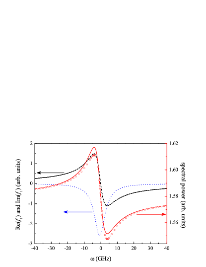
Figure 5: (Color online) Central part of the dissipative soliton spectra perturbed by $\tilde{f}_{1}\left(\omega\right)$ (solid curve) or $\tilde{f}_{0}\left(\omega\right)$ (open squares) as well as the profiles of $\Re\left(\tilde{f}_{1}\right)$ (dashed curve) and $\Im\left(\tilde{f}_{1}\right)$ (dotted curve) from Eq. (12). Single absorption line is centered at $\omega=$0; $\epsilon=-0.005$; $\Omega=4$ GHz.

The pulse spectrum (solid curve in Fig. 5), results from interference of the perturbation with the soliton. For the chosen parameters of the absorption line the zero-order approximation $\tilde{f}_{0}\left(\omega\right)$ (open squares) is very close to the first-order approximation (solid curve) but is slightly down-shifted in the vicinity of the bend maximum and minimum.

With even narrower line width $\Omega$ of 1 GHz (Fig. 6) the spectral perturbation gets very close to the real part of absorber permittivity and, simultaneously, the spectral down-shift $\theta$ (location of the $\Im\left(\tilde{f}_{1}\right)$ minimum, dashed curve) vanishes. The $\tilde{f}_{0}\left(\omega\right)$ (gray solid curves) now perfectly matches the $\tilde{f}_{1}\left(\omega\right)$ (open circles and crosses) within a broad range of $\epsilon$ (gray solid curves 1 and 2 as well as circles and crosses belong to $\epsilon=$-0.005 and -0.05, respectively). The bend amplitudes are in agreement with Eq. (11).

A superposition of three identical absorption lines, which corresponds to the numerical spectra in Fig. 2, is shown in Fig. 7. One can see, that the lowest-order analytical solution $\tilde{f}_{0}\left(\omega\right)$accurately reproduces the numerical result. It is important, that a cumulative contribution of lines into $k\left(\omega\right)$ does not distort a superposition contribution of $S\left(\omega\right)$ into a soliton spectrum (see Eqs. (11,12)). This means that the individual contribution of a single line within a group is easily distinguishable and can be quantitatively assessed, opening way for interesting spectroscopic applications.

As Figs. 5 and 6 suggest, the zero-order approximation $\tilde{f}_{0}\left(\omega\right)=S\left(\omega\right)/\left[k\left(\omega\right)-q\right]$ is quite accurate for a description of perturbation in the limit of $\left|\epsilon\right|\ll 1$. This allows expressing the perturbed spectrum of an isolated line (see (11,12)) in analytical form maple :

$$\tilde{P}(\omega)\equiv\left|\tilde{a}\left(\omega\right)+\tilde{f}_{0}\left(\omega\right)\right|^{2}\approx\frac{A_{0}^{2}\pi^{2}T_{0}^{2}\mathrm{sech}\left(\frac{\pi T_{0}\omega}{2}\right)^{2}\left(\frac{\beta_{2}}{2}\omega^{2}+q\right)^{2}\left(1+\frac{\left(\omega-\omega_{l}\right)^{2}}{\Omega_{l}^{2}}\right)}{\left[\epsilon_{l}^{2}+\frac{2\left(\omega-\omega_{l}\right)\epsilon_{l}}{\Omega_{l}}\left(\frac{\beta_{2}}{2}\omega^{2}+q\right)+\left(\frac{\beta_{2}}{2}\omega^{2}+q\right)^{2}\left(1+\frac{\left(\omega-\omega_{l}\right)^{2}}{\Omega_{l}^{2}}\right)\right]}.$$ (13)

Eq. (13) allows further simplification in the case of $\left|\epsilon\right|\ll 1$

$$\tilde{P}(\omega)\approx A_{0}^{2}\pi^{2}\mathrm{sech}\left(\sqrt{\frac{\alpha}{\sigma}}\frac{\pi\omega}{2}\right)^{2}\frac{\alpha}{\sigma}\left[1+\frac{2\epsilon_{l}\kappa}{\gamma\left(\alpha\omega_{l}^{2}+\sigma\right)}\frac{\left(\omega-\omega_{l}\right)}{\left(1+\frac{\left(\omega-\omega_{l}\right)^{2}}{\Omega_{l}^{2}}\right)\Omega_{l}}\right],$$ (14)

where Eqs. (6) and the condition $\alpha\Omega_{l}^{2}\ll 1$ have been used.

Eq. (14) demonstrates that the spectral bend follows the real part of absorber permittivity. Spectral downshift of bend is the effect of $\mathcal{O}\left(\epsilon^{2}\right)$ and is not included in (14). The perturbation is represented by the term in square brackets and its relative amplitude is proportional to $\epsilon$. Furthermore, the aspect ratio of the kink grows with i) the increase of the relative contribution of the SAM $\kappa/\gamma$ ; ii) the gain bandwidth $1/\sqrt{\alpha}$; iii) approaching of the resonance frequency $\omega_{l}$ to the center of soliton spectrum (but the ratio of the aspect ratio to the local soliton spectral power increases with $\left|\omega_{l}\right|$, because the former decreases as $\omega_{l}^{-2}$ while the latter falls faster as $\cosh\left(\pi T_{0}\omega_{l}/2\right)^{2}$); and iv) with an approaching to the soliton stability border, which corresponds to vanishing $\sigma$. It should be noted, that smaller $\sigma$ entails the soliton width growth (Eq. (6)).

Since the soliton parameters are interrelated, it is instructive to express $\sigma$ through the observable parameters such as soliton energy $E$ or the soliton width $T_{0}$. When $\alpha\omega_{l}^{2}\ll\sigma$ (e.g. $\omega_{l}\approx$0 or/and an oscillator operates far from the stability border $\sigma=$0), the perturbation amplitude is inversely proportional to $\gamma\kappa E^{2}$:

$$\frac{2\epsilon_{l}\kappa}{\gamma\left(\alpha\omega_{l}^{2}+\sigma\right)}\approx\frac{32\epsilon_{l}\alpha}{\gamma\kappa E^{2}}=\frac{2\epsilon_{l}\kappa T_{0}^{2}}{\gamma\alpha}$$ (15)

For a fixed gain bandwidth, the amplitude scales with squared pulsewidth $T_{0}^{2}$. Ultimately, the latter equation is equivalent to

$$\frac{2\epsilon_{l}\kappa}{\gamma\left(\alpha\omega_{l}^{2}+\sigma\right)}\approx-\frac{2\epsilon_{l}}{q},$$ (16)

i.e. the relative perturbation amplitude near soliton central frequency is the ratio of incurred loss coefficient to the soliton wavenumber, regardless of the $z$ coordinate normalization. Therefore, this analytical expression that has been derived for the self-consistent oscillator, should also be valid for the case of a soliton propagation in a long fiber when the conditions of applicability $\left|\epsilon\right|\ll 1$, $\Omega_{l}\ll 1/T_{0}$ are met. The final form of the soliton spectrum thus becomes

$$\tilde{P}(\omega)=\tilde{P}_{0}(\omega)\left(1-\frac{2}{q}\sum_{l}\epsilon_{l}\frac{\left(\omega-\omega_{l}\right)/\Omega_{l}}{1+\frac{\left(\omega-\omega_{l}\right)^{2}}{\Omega_{l}^{2}}}\right),$$ (17)

where $\tilde{P}_{0}(\omega)$ is the spectrum of an unperturbed soliton.

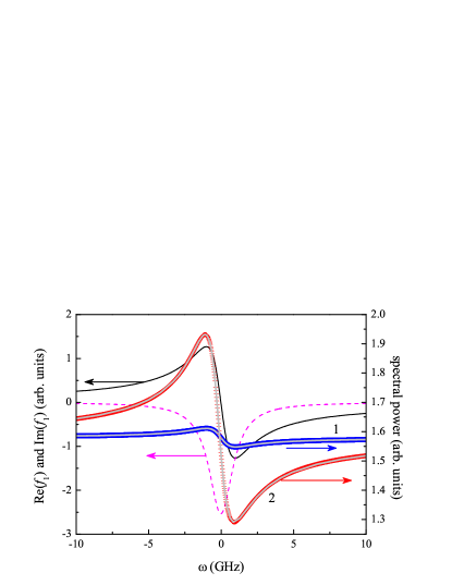
Figure 6: (Color online) Central part of the dissipative soliton spectra perturbed by $\tilde{f}_{1}\left(\omega\right)$ (open circles and crosses) or $\tilde{f}_{0}\left(\omega\right)$ (solid gray curves) as well as the profiles of $\Re\left(\tilde{f}_{1}\right)$ (solid black curve) and $\Im\left(\tilde{f}_{1}\right)$ (dashed curve) from Eq. (12). Single absorption line with $\Omega=1$ GHz is centered at $\omega=$0; $\epsilon=-0.005$ (black solid and dashed curves as well as open circles and solid gray curve 1) and $\epsilon=-0.05$ (crosses and solid gray curve 2).

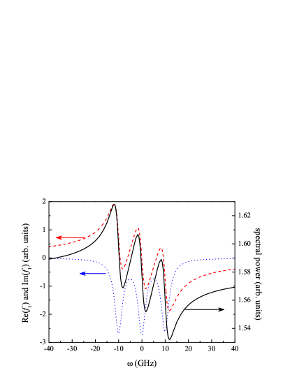
Figure 7: (Color online) Central part of the dissipative soliton spectra perturbed by $\tilde{f}_{0}\left(\omega\right)$ (black solid curve) and the profiles of $\Re\left(\tilde{f}_{0}\right)$ (dashed curve) and $\Im\left(\tilde{f}_{0}\right)$ (dotted curve) from Eq. (12). Triplet of absorption lines is centered at $\omega_{1}=-$10, $\omega_{2}=$0, and $\omega_{3}=$10 GHz; $\epsilon_{1}=\epsilon_{2}=\epsilon_{3}=-0.005$, $\Omega_{1}=\Omega_{2}=\Omega_{3}=2$ GHz.

V Discussion

In the analysis above we have shown that, for the case of sufficiently sparse, narrow and weak Lorentzian absorber lines, their spectral signatures are equivalent to the dispersion-like modulation with a relative amplitude equal to the peak absorption coefficient over oscillator round-trip (or nonlinear length for passive propagation) divided by the soliton wavenumber. For quantitative comparison with the experiment we recall equation (6) and express the maximum spectrum deviation of a single line at $|\omega-\omega_{l}|=\Omega_{l}$ through observable parameters:

$$\left|\frac{\epsilon_{l}}{q}\right|=\chi_{l}L\frac{T_{0}^{2}}{|\beta_{2}|}=\chi_{l}L\frac{0.0319}{|\beta_{2}|(\Delta\nu)^{2}},$$ (18)

where $\chi_{l}=2\epsilon_{l}$ is the peak absorption coefficient of the line, $L$ is the absorber path length and $\Delta\nu$ is the full width at half maximum of the soliton spectrum. Substituting the actual values of the setup in Fig. 1 ($\beta_{2}=-820\pm 40$ fs², $\Delta\nu=$113 cm^-1= 3.39 THz, round-trip air path length $L=149$ cm, relative humidity $50\pm 1$% at $21\pm 0.5$ ^∘C) and taking e.g. the line at 4088 cm^-1 (122.56 THz, marked with an asterisk), we obtain $|\epsilon/q|=0.33\pm 0.02$ for the maximum modulation, which is in perfect agreement with the observed value of 31.5% (Fig. 1b, black line). The agreement is remarkably accurate given the less than optimal resolution of the spectrometer (0.25 cm^-1) and significant third-order dispersion of about +10⁴ fs³ that was not accounted for in the presented analysis.

It is important to notice, that the expression (18) includes only the externally observable soliton bandwidth and relatively stable dispersion parameter. The alignment-sensitive values like saturated losses $\sigma$, nonlinearity $\gamma$, nonlinearity saturation parameter $\kappa$, etc. which are in practice not known with sufficient accuracy, are all accounted for by the self-consistent soliton parameters.

Another important point is the fact, that the signal amplitude $2|\epsilon/q|$ can be much bigger than that from conventional absorption spectroscopy $\chi_{l}L$ of the cell with the same length. The signal enhancement factor can be controlled by the pulse parameters and it exceeds an order of magnitude for the presented case ($\chi_{l}L=5\%$ for selected line and a single-pass cell of a resonator size). For additional sensitivity improvement one can apply the well-developed intracavity multi-pass cell technique multi . The expression (18) suggests, that ultimate sensitivity can be obtained at the expense of the reduced bandwidth coverage $\Delta\nu$. In this respect, the presented technique has the same quadratic dependence of sensitivity on spectral bandwidth as the conventional intracavity absorption spectroscopy ICLAS-gen .

Further refinement of the presented theory should include demonstration of its applicability to arbitrarily shaped absorption features. The superposition property provides a strong argument for such extension, but it has to be rigorously proven for Doppler- and more general Voigt-shaped lines, and also for the dense line groups in e.g. Q-branches. It would be interesting also to extend the theory to the absorber lines at the soliton wings (Fig. 1a).

With the above issues resolved, the soliton-based spectroscopy may become a powerful tool for high-resolution, high-sensitivity spectroscopy and sensing. Possible implementation include soliton propagation in a gas-filled holey fibers, as well as already presented intracavity spectroscopy with femtosecond oscillators. The latter, being a natural frequency comb source, allows direct locking to optical frequency standards, providing for ultimate resolution and spectral accuracy.

VI Conclusion

We have been able to derive an analytical solution to the problem of an one-dimensional optical dissipative soliton propagating in a medium with narrowband absorption lines. We predict appearance of spectral modulation that follows the associated index of refraction rather than absorption profile. The novel perturbation analysis technique is based on integral representation in the spectral domain and is insensitive to the diverging differential terms, inherent to the Taylor series representation of the narrow spectral lines.

The model is applicable to a conventional soliton propagation and to a passively modelocked laser with intracavity absorber, the only difference being the characteristic propagation distance (dispersion length and cavity round-trip, respectively). In the latter case the prediction has been confirmed for a case of water vapour absorption lines in a mid-IR Cr:ZnSe oscillator. The model provides very good qualitative and quantitative agreement with experimental observations, opening a way to metrological and spectroscopical applications of the novel technique, which can provide a significant (order of magnitude and more) enhancement of the signal over conventional absorption for the same cell length.

- (1) E. Sorokin, I.T. Sorokina, J. Mandon, G. Guelachvili, N. Picqué, Opt. Express 15, 16540 (2007).
- (2) J. Mandon, G. Guelachvili, I. Sorokina, E. Sorokin, V. Kalashnikov, N. Picqué, paper WEoB.4 at Europhoton 2008, Europhysics Conference Abstract Volume 32G.
- (3) V. Kalashnikov, E. Sorokin, J. Mandon, G. Guelachvili, N. Picqué, I. T. Sorokina, paper TUoA.3 at Europhoton 2008, Europhysics Conference Abstract Volume 32G.
- (4) I. T. Sorokina , E. Sorokin, T. Carrig, paper CMQ2 at CLEO/QELS 2006, Technical Digest on CD.
- (5) V.M. Baev, T. Latz, P.E. Toschek, Appl. Phys. B. 69, 171 (1999).
- (6) N. Picqué, F. Gueye, G. Guelachvili, E. Sorokin, I.T. Sorokina, Opt. Lett. 30, 3410 (2005).
- (7) The HITRAN database http://www.cfa.harvard.edu/hitran/
- (8) H.A.Haus, J.G.Fujimoto, E.P.Ippen, “Structures for additive pulse mode locking”, JOSA B 8, 2068–2076 (1991).
- (9) N.N.Akhmediev, A.Ankiewicz, Solitons: Nonlinear Pulses and Beams (Chapman&Hall, 1997).
- (10) I.S.Aranson, L.Kramer, Rev. Mod. Phys. 74, 99 (2002).
- (11) T. Brabec, F. Krausz, Phys. Rev. Lett. 78, 3282 (1997).
- (12) F.X.Kärtner (Ed.), Few-cycle Laser Pulse Generation and its Applications (Springer Verlag, Berlin, 2004).
- (13) N.N.Akhmediev, A.Ankiewicz, (Eds.), Dissipative Solitons (Springer Verlag, Berlin, 2005).
- (14) the signs before in Eq. (1) correspond to those in Haus-apm and S.A.Akhmanov, V.A. Vysloukh, A.S.Chirkin, Optics of Femtosecond Laser Pulses (AIP, NY, 1992).
- (15) G.P.Agrawal, Nonlinear Fiber Optics (Academic Press, San Diego, 2001).
- (16) A.Biswas, S.Konar, Introduction to non-Kerr Law Optical Solitons (Chapman&Hall, Boca Raton, 2007).
- (17) H.A.Haus, Y.Silberberg, J. Opt. Soc. Am. B 2, 1237 (1985).
- (18) V.L.Kalashnikov, E.Podivilov, A.Chernykh, A.Apolonski, Applied Physics B 83, 503 (2006).
- (19) V.S.Butylkin, A.E.Kaplan, Yu.G.Khronopulo, E.I.Yakubovich, Resonant Nonlinear Interactions of Light with Matter (Springer Verlag, Berlin, 1989).
- (20) K.E.Oughstun, Electromagmetic and Optical Pulse Propagation 1 (Springer, NY, 2006).
- (21) D.De Sousa Meneses, G.Gruener, M.Malki, P.Echegut, J. Non-Crystalline Solids 351, 124 (2005).
- (22) Y.Yamaoka, L. Zeng, K. Minoshima, H. Matsumoto, Appl. Opt. 43, 5523 (2004).
- (23) M.N. Islam, E.R. Sunderman, C.E. Soccolich, I. Bar-Joseph, N. Sauer, T.Y. Chang, B.I. Miller, IEEE J. Quantum Electron. 25, 2454 (1989)
- (24) U. Keller, K. J. Weingarten, F. X. Kärtner, D. Kopf, B. Braun, I. D. Jung, R. Fluck, C. Honninger, N. Matuschek, J. Aus der Au. IEEE J. Selected Topics in Quantum Electron. 2, 435 (1996).
- (25) V.L.Kalashnikov, Maple worksheet (unpublished) http://info.tuwien.ac.at/kalashnikov/perturb1.html
- (26) A.M. Kowalevicz, A. Sennaroglu, A.T. Zare, J.G. Fujimoto, J. Opt. Soc. Am. B 23, 760 (2006).