PLANAR VISIBILITY: TESTING AND COUNTING

Abstract

In this paper we consider query versions of visibility testing and visibility counting. Let $S$ be a set of $n$ disjoint line segments in $\mathbb{R}^{2}$ and let $s$ be an element of $S$. Visibility testing is to preprocess $S$ so that we can quickly determine if $s$ is visible from a query point $q$. Visibility counting involves preprocessing $S$ so that one can quickly estimate the number of segments in $S$ visible from a query point $q$.

We present several data structures for the two query problems. The structures build upon a result by O’Rourke and Suri (1984) who showed that the subset, $V_{S}(s)$, of $\mathbb{R}^{2}$ that is weakly visible from a segment $s$ can be represented as the union of a set, $C_{S}(s)$, of $O(n^{2})$ triangles, even though the complexity of $V_{S}(s)$ can be $\Omega(n^{4})$. We define a variant of their covering, give efficient output-sensitive algorithms for computing it, and prove additional properties needed to obtain approximation bounds. Some of our bounds rely on a new combinatorial result that relates the number of segments of $S$ visible from a point $p$ to the number of triangles in $\bigcup_{s\in S}C_{S}(s)$ that contain $p$.

1 Introduction

Let $S$ be a set of $n$ closed line segments whose interiors are pairwise disjoint. Two points $p,q\in\mathbb{R}^{2}$ are (mutually) visible with respect to $S$ if the open line segment $pq$ does not intersect any element of $S$. A segment $s\in S$ is visible (with respect to $S$) from a point $p$ if there exists a point $q\in s$ such that $p$ and $q$ are visible. If two objects (points, segments) $A$ and $B$ are visible (with respect to $S$), then we say that $A$ and $B$ see each other (w.r.t. $S$). In this paper we consider the following two problems:

Problem 1 (Visibility testing).

Given a query point $p$ and a segment $s\in S$, determine if $p$ sees $s$.

Problem 2 (Visibility counting).

Given a query point $p$, report the number of segments of $S$ visible from $p$.

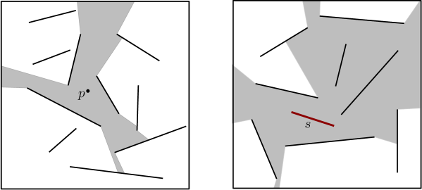
For a point $p\in\mathbb{R}^{2}$, the visibility region or visibility polygon of $p$ (w.r.t. $S$) is defined as (see Figure 1.a):

$$V_{S}(p)=\{q\in\mathbb{R}^{2}:\mbox{$p$ and $q$ are visible (w.r.t. $S$)}\}\enspace.$$

The visibility region of a point is star-shaped, has $p$ in its kernel, and has size $O(n)$. It can be computed in $O(n\log n)$ time by sorting the endpoints of segments in $S$ radially around $p$ and then processing these in order using a binary search tree that orders segments by the order of their intersections with a ray emanating from $p$ [4, 18]. (Equivalently, one can compute the lower-envelope of $S$ in the polar coordinate system whose origin is $p$.) Because $V_{S}(p)$ is star-shaped with $p$ in its kernel it is easy to determine if a query point $q$ is contained in $V_{S}(p)$ in $O(\log n)$ time using binary search. In this way, one can consider $V_{S}(p)$ as an $O(n)$ sized data structure that can test, in $O(\log n)$ time, if a query point $q$ sees $p$.

For a segment $s\in S$, the visibility region of $s$ (with respect to $S$)

$$V_{S}(s)=\bigcup_{q\in s}V_{S}(q)=\{p\in\mathbb{R}^{2}:\mbox{$s$ and $p$ are visible (w.r.t. $S$)}\}$$

is the set of points in $\mathbb{R}^{2}$ that see (at least some of) $s$, see Figure 1.b. Unlike the visibility region of a point, the visibility region of a segment is a complicated structure. For a segment $s$, $V_{S}(s)$ can have combinatorial complexity $\Omega(n^{4})$ and $\mathbb{R}^{2}\setminus V_{S}(s)$ can have $\Omega(n^{4})$ connected components [16, Figure 8.13][10, Lemma 12], see also Figure 2.

More troublesome than the worst-case complexity of $V_{S}(s)$ is that there exist sets $S$ of $n$ line segments where, for most of the elements $s\in S$, the complexity of $V_{S}(s)$ is $\Omega(n^{2})$. Therefore, explicitly computing $V_{S}(s)$ and preprocessing it for point location does not yield a particularly space-efficient data structure for testing if a query point $p$ sees $s$, even if $s$ is a “typical” (as opposed to worst-case) element of $S$.

In this paper we propose efficient data structures that use an old result of Suri and O’Rourke [18] which shows that $V_{S}(s)$ can be represented as a set of $O(n^{2})$ triangles whose union is $V_{S}(s)$. We define a variant of their covering, give efficient algorithms for computing it, and prove additional properties of the covering. In particular, we define a covering $C_{S}(s)$ of $V_{S}(s)$ by triangles. We prove that for a randomly chosen $s\in S$, the expected size of $C_{S}(s)$ is $O(n)$. This, of course, implies that $|\bigcup_{s\in S}C_{S}(s)|=O(n^{2})$. Additionally, if we define $C(S)=\bigcup_{s\in S}C_{S}(s)$, then we prove that the number of triangles of $C(S)$ containing any point $p$ is a $2$-approximation to the number of segments of $S$ visible from $p$.

Applications of these results include efficient data structures for testing if a query point is contained in $V_{S}(s)$ as well as efficient data structures for estimating the number of points of $S$ visible from a query point. In order to express our results more precisely, we need some further definitions.

Figure 1: (a) The visibility region for a point and (b) The visibility region of a line segment.

1.1 Visibility Graphs and Extended Visibility Graphs

The visibility graph $\mathit{VG}(S)$ is a graph whose vertices are the $2n$ endpoints of the segments in $S$ and in which the edge $pq$ exists if and only if the open line segment with endpoints $p$ and $q$ does not intersect any (closed) segment in $S$. (see Figure 3.a). It is well-known that the number of edges $m$ of $\mathit{VG}(S)$ is in $O(n^{2})$. Ghosh and Mount [12] give an optimal $O(n\log n+m)$ time algorithm to compute the visibility graph of a set of $n$ disjoint line segments. Here, and throughout the remainder of the paper, $m=m(S)$ is the number of edges of $\mathit{VG}(S)$.

Figure 2: An example of a set $S$ where $V_{S}(s)$ has complexity $\Omega(n^{4})$. The $O(n)$ segments in the center define $\Omega(n^{2})$ visibility graph edges whose extensions intersect in $\Omega(n^{4})$ points.

Assume, w.l.o.g., that no segment in $S$ is vertical, so we can say that a point $p$ is above a segment $s\in S$ if $p$ is above the line that contains $s$. Assume, furthermore, that $S$ contains four segments that define a rectangle that contains all the elements of $S$ in its interior. The first assumption can be ensured by performing a symbolic rotation of $S$. The second assumption is only used to ensure that all visibility regions that we discuss are bounded.

The extended visibility graph $\mathit{EVG}(S)$ is obtained by adding $2m$ edges and at most $2m$ vertices to $\mathit{VG}(S)$ as follows (see Figure 3.b): For each (directed) edge $uv$ in $\mathit{VG}(S)$, extend a segment $e_{uv}$ from $v$ in the direction $\overrightarrow{uv}$ until it intersects an element of $S$ at some point $w$. If not already present, then add the vertex $w$ to $\mathit{EVG}(S)$ and add the edge $vw$ to $\mathit{EVG}(S)$. The extended visibility graph can be computed in $O(n\log n+m)$ time using the visibility graph algorithm by Ghosh and Mount [12].

The union of the edges of $\mathit{EVG}(S)$ and the segments in $S$ form a 1-dimensional set whose removal disconnects $\mathbb{R}^{2}$ into a set of 2-dimensional regions. This set of 2-d regions is known as the visibility space partition, $\mathit{VSP}(S)$ of $S$. The regions of $\mathit{VSP}(S)$ are important because for any region $R\in\mathit{VSP}(S)$ and for any $p,q\in R$ the set of segments of $S$ visible from $p$ is equal to the set of segments of $S$ visible from $q$. The region of $\mathit{VSP}(S)$ that contains $p$ determines all the combinatorial information about $V_{S}(p)$.

Note that $\mathit{VSP}(S)$ is defined by $O(n^{2})$ lines, rays, and segments and therefore has worst-case complexity $O(n^{4})$.

(a)	(b)

Figure 3: The visibility graph and the extended visibility graph of a set of seven line segments. (Segments are bold, graph edges are dashed.)

1.2 Previous Work

There is a plethora of work on visibility in the plane. This section discusses only some of the work most relevant to the current paper.

The visibility space partition is bounded by a subset of the $O(n^{2})$ lines induced by pairs of endpoints in $S$. The $\mathit{VSP}(S)$ has complexity $O(m^{2})$ where $m$ is the number of edges in $\mathit{VG}(S)$ and can be computed in $O(m^{2})$ time after constructing $\mathit{VG}(S)$ using standard algorithms.

By preprocessing $\mathit{VSP}(S)$ with a point location structure and augmenting the regions of $S$ with appropriate information, one obtains an $O(m^{2})$ size data structure that can answer visibility testing queries and visibility counting queries in $O(\log n)$ time.

If the segments of $S$ are the edges of a simple polygon then Bose et al. [5] and Guibas et al. [13] show that the complexity of $\mathit{VSP}(S)$ is only $O(n^{3})$. In this case, this immediately solves the two problems using a structure of size $O(n^{3})$. Aronov et al. [3] give a data structure that reduces the space to $O(n^{2})$ but increases the $O(\log n)$ query time term to $O(\log^{2}n)$, again for the case where segments of $S$ are the edges of a simple polygon.

Pocchiola and Vegter [17] give an $O(m)$ space data structure, the visibility complex, that can compute the visibility polygon $V_{S}(p)$ from any query point $p$ in $O(m_{p}\log n)$ time, where $m_{p}$ is the complexity of $V_{S}(p)$. When the segments of $S$ define a polygon with $h$ holes then Zarei and Ghodsi [19] give an $O(n^{3})$ space data structure that can compute the visibility polygon $V_{S}(p)$ in $O(m_{p}\log n)$ time and the query time of their structure is $O(\min\{h,m_{p}\}\log n+m_{p})$, which improves the query time of Pocchiola and Vegter when $h\ll m_{p}$.

Motivated by the computer graphics problem of estimating a priori the savings to be had by applying a visibility culling algorithm, Fischer et al. [10, 11] give approximation algorithms for Problem 2. They present two approximation data structures for visibility counting. One structure uses a $(r/m)$-cutting [15, Section 4.5] of the $\mathit{EVG}(S)$ to obtain a data structure of size $O((m/r)^{2})$ that answers queries in $O(\log n)$ time and approximates the visibility count up to an absolute error of $r$. Another structure uses random sampling to obtain a data structure of size $(m^{2}\log^{O(1)}n)/\ell$, that has query time $\ell\log^{O(1)}n$, and that approximates the visibility count up to an absolute error of $\delta n$ for any constant $\delta>0$. (Note that $\delta$ affects the leading constants of both the query time and space requirements.)

1.3 New Results

In the current paper we revisit O’Rourke and Suri’s proof that, for any $s\in S$, there exists a set $C_{S}(s)$ of $O(m_{s})$ triangles whose union is $V_{S}(s)$, where $m_{s}$ is the number of edges of $\mathit{EVG}(S)$ incident on $s$. We show that this covering has the additional property that if we take the $O(m)$ size set $C(S)=\bigcup_{s\in S}C_{S}(s)$ of triangles, then the number of triangles containing any point $p\in\mathbb{R}^{2}$ is a $2$-approximation to the number of segments of $s$ that are visible from $p$.

These triangle-covering results have several applications that are obtained by storing the resulting triangles in a layered partition tree. Here, and throughout the remainder of the paper, $\epsilon>0$ is a constant that can be made arbitrarily small. To reduce clutter, we use the notation $O_{\epsilon}(f(n))=O(f(n)n^{\epsilon})$.

1.3.1 Visibility testing

By storing the elements of $C_{S}(s)$ in a partition tree, we obtain, for any $k$ with $m_{s}\leq k\leq m_{s}^{2}$, an $O(k)$ space data structure that can test, in $O_{\epsilon}(m_{s}/\sqrt{k})$ time, if a query point $p$ is contained in $V_{S}(s)$. Barring a major breakthrough on Hopcroft’s Problem [8], this result is likely only a factor of $O(n^{\epsilon})$ from the optimal. See Section 3.1.

For comparison, the best previously described structure for this problem, as used within the results of Fischer et al. [10, 11], has size $O(m_{s}^{2}/\ell)$ and answers queries in $O(\ell\log n)$ time, where $\ell\geq 1$ is a space/time tradeoff parameter of the data structure. Taking $\ell=\sqrt{n}$ yields a space of $O(m_{s}^{3/2})$ and a query time of $O(\sqrt{m_{s}}\log n)$. On the other hand, taking $k=m_{s}^{3/2}$ in our data structure yields an $O(m_{s}^{3/2})$ space data structure with query time $O_{\epsilon}(m_{s}^{1/4})$.

1.3.2 Visibility Counting — Relative Approximation

By putting all the triangles of $C(S)$ into a partition tree, we obtain a data structure that can $2$-approximate the number of segments of $S$ visible from any query point. For any $k$ with $m\leq k\leq m^{2}$, this structure has size $O(k)$ and answers queries in time $O(m/\sqrt{k})$. The structure returns a visibility count $m^{\prime}_{p}$ that satisfies $m_{p}\leq m^{\prime}_{p}\leq 2m_{p}$. See Section 3.2.

1.3.3 Visibility Counting — Absolute Approximation

Using a selective random sampling of the segments in $S$, we obtain a data structure of size $O_{\epsilon}((cm/n)(cn)^{\alpha})=O_{\epsilon}(n^{1+\alpha})$ that approximates the number of segments of $S$ visible from any query point in time $O_{\epsilon}(c(m/n)^{(1/2)(1-\alpha)})=O_{\epsilon}(cn^{(1/2)(1-\alpha)})$, for any given constants $c,\delta>0$ and $0\leq\alpha\leq 1$. With probability at least $1-n^{\Omega(\delta^{2}cn/m_{p})}$, the structure returns a value $m^{\prime\prime}_{p}$ such that $m_{p}-c/n-\delta n\leq m^{\prime\prime}_{p}\leq m_{p}+\delta n$. This data structure is described in Section 3.3.1.

Using random sampling in a different manner, we obtain a space versus query time tradeoff. For any $k$ with $m/n\leq k\leq(m/n)^{2}$, we obtain a structure of size $O_{\epsilon}(k)$ and query time $O_{\epsilon}(m/(n{\sqrt{k}}))$. This structure returns a visibility count $m^{\prime\prime}_{p}$ that satisfies $m_{p}-\delta n\leq m^{\prime\prime}_{p}\leq 2m_{p}+\delta n$. The details can be found in Section 3.3.2.

(a)	(b)	(c)

Figure 4: The algorithm for covering $V^{+}_{S}(s)$ with triangles processes the events at (a) $p_{1}$, (b) $p_{2}$ and (c) $p_{3}$. Active edges are shown in orange and triangles in the covering are shown at the time they are added to the covering.

These results compare favourably with those of Fischer et al. [10, 11]. Their cutting-based data structure, with parameter $r=\delta n$, gives an absolute error of $\delta n$, uses space $O((m/n)^{2})$ and has a query time of $O(\log n)$. Their random sampling-based data structure, with parameter $\ell=\sqrt{n}$, gives a data structure of size $(m^{2}\log^{O(1)}n)/\sqrt{n}$ with query time $\sqrt{n}\log^{O(1)}n$.

The remainder of the paper is organized as follows: Section 2 proves results on covering visibility regions with triangles. Section 3 applies these results to obtain new results on visibility testing and counting. Section 4 summarizes and concludes with open problems.

2 Covering $V_{S}(s)$

In this section we give an algorithm for covering the visibility region $V_{S}(s)$ with a set $C_{S}(s)$ of triangles. The resulting covering is similar to the covering given by Suri and O’Rourke [18], the main difference being around the triangles adjacent to the endpoints of $s$. However, our exposition, and our algorithm for computing $C(S)$ are more $s$-centric. This leads to efficient output-sensitive algorithms for constructing $C_{S}(s)$, rather than the worst-case optimal $O(n^{2})$ algorithm obtained by Suri and O’Rourke [18]. The number of triangles used in $C_{S}(s)$ is bounded by $O(m_{s})$ where $m_{s}$ is the number of edges of $\mathit{EVG}(S)$ that are incident to $s$.

We will show how to cover the portion $V^{+}_{S}(s)\subseteq V_{S}(s)$ in the halfplane bounded from below by the supporting line of $s$ with a set $C^{+}_{S}(s)$ of triangles. The complementary part $V^{-}_{S}(s)=V_{S}(s)\setminus V^{+}_{S}(s)$ can be covered with a set $C^{-}_{S}(s)$ using a symmetric algorithm.

The covering algorithm works by sweeping a point $p$ from left to right along the segment $s$. Events in this sweep occur at the vertices $p_{1},\ldots,p_{m^{\prime}_{s}}$ of $\mathit{VSP}(S)$ incident on $s$, in their left to right order, so that $p_{1}$ and $p_{m^{\prime}_{s}}$ are the left and right endpoints, respectively, of $s$.

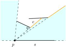
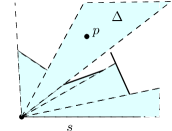
Let $e$ be an edge of $V^{+}_{S}(p)$ that is collinear with $p$ and such that the interior of $V^{+}_{S}(p)$ is to the right of $e$. We call such an edge an active edge of $V^{+}_{S}(p)$. Active edges are important because, as $p$ moves to the right, they uncover regions of $\mathbb{R}^{2}$ which may not have been previously visible. See Figure 4.a.

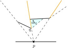
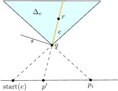
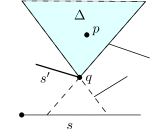
Let $q$ be the lower endpoint of an active edge $e$ and note that $q$ is an endpoint of some segment in $S$. Consider what happens to $e$ as the viewpoint $p$ moves left to right along $s$, but does not cross any edge of $\mathit{EVG}(S)$ collinear with $q$. As $p$ moves left to right, the edge $e$ remains collinear with $p$ and $q$ and sweeps over a triangle $\Delta_{e}$ whose lowest vertex is $q$. This continues until the point $p$ reaches an edge of $\mathit{VSP}(S)$ incident on $q$. See Figure 4.b.

Algorithmically, the cover $C^{+}_{S}(s)$ is constructed as follows: Initially $p=p_{1}$ is the left endpoint of $S$. We compute the visibility polygon $V^{+}_{S}(p)$, whose boundary is a sequence of $2m_{p}=O(n)$ edges that alternate between subsegments of the elements of $S$ and segments collinear with $p$ and an endpoint of an element of $S$. This polygon can be covered in a natural way with $m_{p}$ non-overlapping triangles, each of which has $p$ as a vertex (see Figure 4.a). These $m_{p}$ triangles are added to $C^{+}_{S}(s)$. After computing $V^{+}_{S}(p)$ we identify its active edges, and with each active edge $e$ we store the value $\operatorname{start}(e)=p_{1}$.

Next, we sweep $p$ from left to right, pausing at the vertices $p_{2},\ldots,p_{m^{\prime}_{s}}$ as we go. Upon reaching a vertex $p_{i}$, we process the edges of $\mathit{EVG}(S)$ incident on $p_{i}$ one at a time. Let $e^{\prime}$ be an edge of $\mathit{EVG}(S)$ incident on $p_{i}$. If $e^{\prime}$ is collinear with an active edge $e$ of $V^{+}_{S}(p)$ then we generate a new triangle $\Delta_{e}$ for $C^{+}_{S}(s)$. The lowest vertex of $\Delta_{e}$ is the lower endpoint $q$ of $e$. $\Delta_{e}$ is bounded by two lines $\ell_{1},\ell_{2}$, both of which contain $q$, and where $\ell_{1}$ contains $p_{i}$ and $\ell_{2}$ contains $\operatorname{start}(e)$. The third side of $\Delta_{e}$ is bounded by the segment in $S$ incident on $e$ and furthest from $p_{i}$. See Figure 4.b.

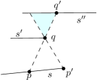
Finally, the visibility polygon $V^{+}_{S}(p)$ is updated in the neighbourhood of $e$, which possibly creates up to two new active edges incident to $q$. Each new active edge $f$ is marked as active and we set $\operatorname{start}(f)=p_{i}$. The exact nature of this update depends on the relative locations of the two segments that define $e^{\prime}$. The three possible cases are illustrated in Figure 7.

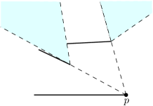
Note that an important event, but which requires no special handling, occurs at the right endpoint of $s$ when $p=p_{m_{s}}$. In this case, each active edge of $V^{+}_{S}(p)$ generates a triangle that is added to the set $C^{+}_{S}(s)$. See Figure 4.c.

We now prove the correctness, construction time and approximation bound of the above algorithm.

Lemma 1.

Let $C^{+}_{S}(s)$ be the set of triangles generated by the above algorithm. Then $\cup C^{+}_{S}(s)=V^{+}_{S}(s)$ and $|C^{+}_{S}(s)|\leq m_{s}$ where $m_{s}$ is the number of edges of $\mathit{VSP}(S)$ incident on $s$.

Proof.

To prove the bound on the size, first observe that the initial visibility polygon $V^{+}_{S}(p_{1})$ has size that is bounded by the degree of $p_{1}$ in $\mathit{VSP}(S)$. Furthermore, at each event point $p_{i}$, $i>1$, the number of triangles added to $C^{+}_{S}(s)$ is at most the number of edges of $\mathit{VSP}(S)$ incident to $p_{i}$. Therefore, the total number of triangles in $C^{+}_{S}(s)$ is at most the number of edges of $\mathit{VSP}(S)$ incident on $s$.

The fact that $\cup C^{+}_{S}(s)\subseteq V^{+}_{S}(s)$ follows immediately from the easily verifiable fact that each triangle added to $C^{+}_{S}(s)$ contains only points visible from some point on $p\in s$. In particular, for any point $r$ in the triangle $\Delta_{e}$ that is added to $V^{+}_{S}(s)$ when processing $p_{i}$, there is a point $q$ in the subsegment of $s$ between $\operatorname{start}(e)$ and $p_{i}$ that sees $r$.

To prove that $C^{+}_{S}(s)$ covers $V^{+}_{S}(s)$, consider a point $r\in V^{+}_{S}(s)$. If $r$ is visible from $p_{1}$ then $r$ is contained in one of the triangles added during the initialization of the algorithm. Otherwise, there exists some point $p^{\prime}\in s$ with minimum $x$-coordinate such that $r$ is visible from $p^{\prime}$. It follows that $p^{\prime}$ and $r$ are collinear with a vertex $q$ of some segment $s^{\prime}\in S$ and that $q$ is on the segment $p^{\prime}r$ (see Figure 5.a). Then $q$ is an endpoint of an active edge $e$ of $V^{+}_{S}(p^{\prime})$ with $\operatorname{start}(e)$ to the left of $p^{\prime}$. Since every active edge eventually adds a triangle to $C^{+}_{S}(s)$, there is some $p_{i}$ to the right of $p^{\prime}$ that adds a triangle $\Delta_{e}$ to $C^{+}_{S}(s)$ that contains $r$ (see Figure 5.b). Since this is true for every point $r\in V^{+}_{S}(s)$, we conclude that $\cup C^{+}_{S}(s)\supseteq V^{+}_{S}(s)$, and hence $\cup C^{+}_{S}(s)=V^{+}_{S}(s)$. ∎

(a)	(b)

Figure 5: Proving that $C^{+}_{S}(s)$ covers $V^{+}_{S}(s)$.

Lemma 2.

Let $S$ be a set of $n$ disjoint line segments. The covering $C_{S}(s)$ can be computed in

1. $O(m_{s})$ time if we are given $\mathit{EVG}(S)$ or

2. $O_{\epsilon}(n+(m_{s}n)^{2/3})$ otherwise.

Proof.

Part 1 of the lemma is clear. The algorithm for constructing $C_{S}(s)$ processes the edges of $\mathit{EVG}(S)$ incident on $s$ in the order in which they appear. These $m_{s}$ edges can be easily extracted from $\mathit{EVG}(S)$ in the order in which they appear and processing each edge takes $O(1)$ time.

Part 2 of the lemma requires some use of a geometric range searching structure for answering ray-sweeping queries. Let $q$ and $q^{\prime}$ be two points that are visible, with $q^{\prime}$ on some segment $s^{\prime\prime}\in S$. A ray-sweeping query asks to determine the first endpoint of a segment in $S$ that is intersected by $qq^{\prime}$ as the point $q^{\prime}$ moves towards the left endpoint of $s^{\prime\prime}$.

A ray-sweeping query is an optimization problem. It’s corresponding decision problem is a triangle interference query, which asks to determine if a query triangle $\Delta$ with vertices $q$, $q^{\prime}$ and $q^{\prime\prime}\in s^{\prime\prime}$ intersects any segment of $S$. Because $q$ and $q^{\prime}$ are visible and $q^{\prime}$ and $q^{\prime\prime}$ are both on $s^{\prime\prime}$, it is not hard to see that if $\Delta$ does intersect some segment in $S$, then $\Delta$ contains an endpoint of a segment in $S$. That is, a triangle interference query can be solved using a triangular range searching structure built on the endpoints of segments in $S$.

Triangular range searching is a well studied problem, and a number of solutions exist that, for any $k$ with $n\leq k\leq n^{2}$, give $O_{\epsilon}(k)$ space structures with $O_{\epsilon}(n/\sqrt{k})$ query time [1, Section 4]. Using one of these structures and applying Chan’s randomized optimization technique [6, Theorem 3.2] yields a data structure for ray-sweeping queries with the same preprocessing, space, and query time bounds.

To construct $C_{S}(s)$ we use essentially the same sweeping algorithm used to define $C_{S}(s)$ except that ray-sweeping queries are used to compute the algorithm’s events on the fly. The algorithm uses a priority queue $Q$ to order and process these event points in left to right order. To initialize the algorithm, we construct the visibility polygon $V_{S}(p=p_{1})$ in $O(n\log n)$ time using a radial sweep [4, 18]. Next, each active edge of $V_{S}(p)$ is identified and processed.

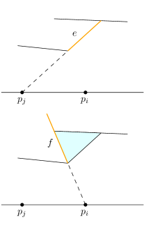
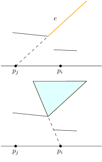
Anytime (during initialization or later) that an active edge $e=qq^{\prime}$ is created, the algorithm performs a ray-sweeping query with the segment $qq^{\prime}$ and a ray sweeping query with the edge $q^{\prime}p$ (see Figure 6). The results of these two queries determine an event point $p^{\prime}\in s$ to the right of $p$ at which time the edge $e$ contributes a triangle $\Delta_{e}$ to $s$. This event point $p^{\prime}$ is enqueued in $Q$. It is not hard to verify that this algorithm computes the same set of triangles $C_{S}(s)$ as the original algorithm and that the number of ray-sweeping queries performed is $O(m_{s})$ (at most two queries are performed for each triangle added to $C_{S}(s)$).

Figure 6: The four cases that can occur when using a ray-sweeping query to determine the point $p^{\prime}$ at which active edge $e=qq^{\prime}$ contributes a triangle to $C_{S}(s)$.

Therefore, the algorithm can be implemented to run in $O_{\epsilon}(k+m_{s}n/\sqrt{k})$ for any $n\leq k\leq n^{2}$. Given the value of $m_{s}$ in advance, setting $k=(m_{s}n)^{2/3}$ would yield the stated time bound. However, even without knowing $m_{s}$ in advance we can begin by estimating the value of $m_{s}$ as $m^{\prime}_{s}=2$ and doubling our estimate (and rebuilding the ray-sweeping structure) if we discover that $m_{s}>m^{\prime}_{s}$. This doubling strategy yields the overall time bound of $O_{\epsilon}(n+(m_{s}n)^{2/3})$, as required. ∎

Next we show that, in a global sense, the number of triangles containing a point $p\in\mathbb{R}^{2}$ gives a $2$-approximation to the number of segments of $S$ that are visible from $p$.

(a)	(b)	(c)

Figure 7: The three cases that occur when processing an edge of $\mathit{EVG}(S)$ incident on $p_{i}$. Here, $\operatorname{start}(e)=p_{j}$.

Lemma 3.

Let $C(S)=\bigcup_{s\in S}C_{S}(s)$ and let $p$ be any point in $\mathbb{R}^{2}$ that is not on the boundary of any triangle in $C(S)$. If $m_{p}$ is the number of segments in $S$ (partially) visible from $p$ and $m^{\prime}_{p}$ is the number of triangles in $C(S)$ that contain $p$, then $m_{p}\leq m^{\prime}_{p}\leq 2m_{p}$.

Proof.

Let $C_{p}\subseteq C(S)$ be the set of triangles in $C(S)$ that contain $p$, and let $S_{p}\subseteq S$ be the set of segments in $S$ that are (partially) visible from $p$. Our goal is to show that $|S_{p}|\leq|C_{p}|\leq 2|S_{p}|$. The lower bound on $m^{\prime}_{p}=|C_{p}|$ is trivial: For every segment $s\in S_{p}$, $V_{S}(s)$ contains $p$, so, by Lemma 1, $C_{S}(s)$ contributes at least one triangle to $C_{p}$.

To prove the upper bound, we describe a mapping $f:C_{p}\rightarrow S_{p}$ that is $2$-to-one; for every $s\in S_{p}$, there exists at most two triangles $\Delta\in C_{p}$ such that $f(\Delta)=s$. The existence of $f$ then proves the upper bound.

Let $\Delta\in C_{p}$ be some triangle that contains $p$ and suppose that $\Delta\in C_{S}(s)$ for some $s\in S$ that is, without loss of generality, below $p$. If $\Delta$ is incident on $s$ (Figure 8.a), then $\Delta$ was added to $C_{S}(s)$ as part of $V_{S}(p)$ where $p$ was the left endpoint of $s$. In this case, we set $f(\Delta)=s$. Otherwise, $\Delta$ was created when sweeping $s$ with $p$ and some active edge $e$ of $V_{S}(p)$ generated $\Delta$ (Figure 8.b). The vertex $q$ of $\Delta$ that is closest to $s$ is incident on a segment $s^{\prime}\in S$. In this case $f(\Delta)=s^{\prime}$.

(a) $f(\Delta)=s$	(b) $f(\Delta)=s^{\prime}$

Figure 8: The mapping $f$ takes $\Delta$ onto (a) $s$ and (b) $s^{\prime}$.

We now argue that $f$ is 2-to-one. Let $s\in S$ be some segment and suppose, without loss of generality, that $p$ is above $s$. Consider a triangle $\Delta\in f^{-1}(s)$ and observe that, by the definition of $f$, $\Delta$ has a vertex that is an endpoint of $s$.

Note that there is at most one triangle in $C_{S}(s)\cap C_{p}$ that maps to $s$, and this triangle exists precisely if $p$ is visible from the left endpoint of $s$. All that remains to show is that there is at most one additional segment $s^{\prime}\in S$, $s^{\prime}\neq s$ such that $C_{S}(s^{\prime})$ contains a triangle $\Delta$ with $f(\Delta)=s$.

Let $\Delta$ be such a triangle and suppose that $\Delta$ is incident to the endpoint $q$ of $s$. Refer to Figure 9. The triangle $\Delta$ was generated by an active edge when processing $s^{\prime}$. In particular, there is a subsegment $p_{j}p_{i}\subseteq s^{\prime}$ such that an active edge $e$ of $V^{+}_{S}(p)$ sweeps over $\Delta$ when $p$ travels from $p_{j}$ to $p_{i}$. (Note, $p_{j}=\operatorname{start}(e)$.) This implies that $p_{i}$ and $p_{j}$ are below $s$. Since $p$ travels from left to right along $e$, this implies that $q$ is the right endpoint of $s$ because, otherwise, $e$ would not be an active edge of $V^{+}_{S}(p)$.

Figure 9: At most one triangle in $f^{-1}(s)$ is incident to the right endpoint of $S$.

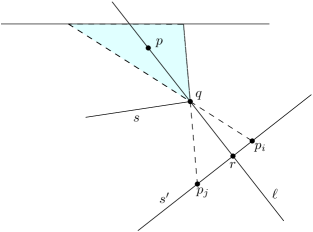
Thus far, we have established that at most one triangle in $f^{-1}(s)$ is incident to the left endpoint of $s$. To see that at most one triangle ($\Delta$, discussed above) is incident to the right endpoint of $s$, suppose by way of contradiction that there are two such triangles $\Delta$ and $\Delta^{\prime}$ with $\Delta\in C_{S}(s^{\prime})$ and $\Delta^{\prime}\in C_{S}(s^{\prime\prime})$. Consider the line $\ell$ through $p$ and $q$. Observe that $\ell$ intersects both $s$ and $s^{\prime}$, in two points $r$ and $r^{\prime}$, respectively. But this is not possible since then one of $r$ or $r^{\prime}$ does not see the endpoint $q$. ∎

Remark:

The condition, in Lemma 3, that $p$ is not on the boundary of any triangle in $C_{S}(s)$ is unnecessary if we take a little extra care. In particular, the mapping $f$ actually maps triangles to the endpoints of segments. The set $C_{S}(v)$ of triangles mapped to a particular endpoint $v$ all have $v$ as a vertex and no two triangles in $C_{S}(v)$ share an interior point. This means that we can define each triangle in $C_{S}(v)$ to either include or exclude some of its edges or vertices so that the triangles are disjoint but their union remains unchanged. This yields a set of (partially open) triangles $C^{\prime}(S)$ for which Lemma 3 holds for any point $p\in\mathbb{R}^{2}$.

3 Applications

In this section, we consider applications of Lemma 1 and Lemma 3 to some visibility testing and counting problems. These applications rely on data structures for triangle inclusion counting: Given a set $T$ of triangles, we want to preprocess $T$ into a data structure for counting the number of triangles in $T$ that contain a query point $p$.

The tools needed to perform these queries are well-known, but finding the relevant structures and techniques, and applying them correctly, can take some time. Therefore, we review the data structure here and point out the relevant references.

Let $\Delta$ be a triangle. Then $\Delta$ is the intersection of at most 4 halfplanes bounded by four lines $h(\Delta)=(u_{1},u_{2},d_{1},d_{2})$ where $u_{1}$ and $u_{2}$ bound $\Delta$ from below and $d_{1}$ and $d_{2}$ bound $\Delta$ from above. Given a triangle $\Delta$ we have either $u_{1}=u_{2}$ or $d_{1}=d_{2}$. By the standard duality mapping [7, Section 8.2] the four lines in $h(\Delta)$ map to four points $u_{1}^{*}$, $u_{2}^{*}$, $d_{1}^{*}$ and $d_{2}^{*}$. A point $p\in\mathbb{R}^{2}$ maps to a line $p^{*}$ in the dual plane. The point $p$ is contained in $\Delta$ if and only if the line $p^{*}$ is above (or on) $u_{1}^{*}$ and $u_{2}^{*}$ and below (or on) $d_{1}^{*}$ and $d_{2}^{*}$. Let $h^{*}(\Delta)=(u_{1}^{*},u_{2}^{*},d_{1}^{*},d_{2}^{*})$.

A triangle inclusion counting structure for $T$ stores the 8-dimensional point-set

$$h^{*}(T)=\{h^{*}(\Delta):\Delta\in T\}\enspace.$$

Given a query point $p$, we want to count the number of points $(a,b,c,d)\in h^{*}(T)$ that satisfy the four requirements:

1. $a$ is above $p^{*}$, and

2. $b$ is above $p^{*}$, and

3. $c$ is below $p^{*}$, and

4. $d$ is below $p^{*}$.

Counting the number of points in $h^{*}(T)$ that satisfy any one of these requirements is a halfplane range counting problem. Data structures for halfplane range counting are plentiful, and there are several data structures known that use $O_{\epsilon}(k)$ space and have query time $O_{\epsilon}(n/\sqrt{k})$ [1, Section 4]. Several of these structures (for example, Matoušek’s efficient partition trees [14]) are hierarchical structures that are efficient and $r$-convergent (see Agarwal and Erickson [1, Section 5] for definitions of hierarchical, efficient, and $r$-convergent). This implies [1, Theorem 10] that there exists a 4-layer structure that uses $O_{\epsilon}(k)$ space and preprocessing time and that, in time $O_{\epsilon}(n/\sqrt{k})$, can count the number of elements in $h^{*}(T)$ that satisfy the constraints 1–4 for any query point $p^{*}$. Translating this back into primal space we obtain the data structure we need:

Theorem 1 ([1, 14]).

Let $T$ be a set of $n$ triangles. For any $k$ with $n\leq k\leq n^{2}$, there exists a data structure of size $O_{\epsilon}(k)$ that can be constructed in time $O_{\epsilon}(k)$ and that can count the number of triangles containing a query point $p$ in $O_{\epsilon}(n/\sqrt{k})$ time.

3.1 Visibility Testing

Our first application follows immediately by storing the triangles of Lemma 1 in the data structure of Theorem 1. This yields our first result:

Theorem 2.

Let $S$ be a set of $n$ disjoint line segments and let $s\in S$ be a special segment. For any $m_{s}\leq k\leq m_{s}^{2}$, there exists a data structure of size $O_{\epsilon}(k)$ that can test, in $O_{\epsilon}(m_{s}/\sqrt{k})$ time, if any query point $p$ is contained in $V_{S}(s)$. The data structure can be constructed in

1. $O_{\epsilon}(k)$ time if we are given $\mathit{EVG}(S)$ or

2. $O_{\epsilon}(n+(m_{s}n)^{2/3}+k)$ time otherwise.

Next we argue that, barring a breakthrough on Hopcroft’s Problem [8], Theorem 2 is near-optimal. Hopcroft’s Problem takes as input a set $L$ of $n$ lines and a set $P$ of $n$ points and asks if any point in $P$ is contained in any line in $L$. Currently, the most efficient methods of solving Hopcroft’s Problem have running times in $\Omega(n^{4/3})$. Furthermore, $\Omega(n^{4/3})$ is a lower bound for Hopcroft’s Problem in a restricted model of computation that can model all known algorithms for the problem [8].

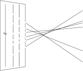
Given the set $L$, we can compute the leftmost intersection point between any pair of lines by sorting the lines by slope and checking the intersection points between consecutive pairs of lines. Assume, without loss of generality, that this leftmost intersection point has $x$-coordinate equal to 0. Using infinitesimal gaps between segments, we can easily construct a set of $3n+O(1)$ segments $s_{0},\ldots,s_{3n+O(1)}$ such that a query point $p$ whose $x$-coordinate is greater than 0 is visible from $s_{0}$ if and only if $p$ lies on one of the lines in $L$ (see Figure 10). For a query point $p$ with $x$-coordinate smaller than 0 we can test if $p$ is contained in any line of $L$ in $O(\log n)$ time by storing the lines of $L$ sorted by slope and using binary search.

(a)	(b)

Figure 10: A set $L$ of lines (a) and a set of $3n+O(1)$ segments where testing if a point is in $V_{S}(s_{0})$ helps to determine if the point is contained in any line of $L$.

Therefore, by the above discussion, setting $k=n^{4/3}$ and using Theorem 2 we can use this data structure to solve Hopcroft’s Problem in $O_{\epsilon}(n^{4/3})$ time. Furthermore, the existence of a data structure for testing if $V_{S}(s)$ contains a query point $p$ that could be constructed in $o(n^{4/3})$ time and whose query time is $o(n^{1/3})$ would give a $o(n^{4/3})$ time algorithm for Hopcroft’s Problem.

3.2 Visibility Counting – Relative Approximation

Next we consider Fischer et al.’s problem of approximate visibility counting [10, 11]. We want to preprocess the segments in $S$, so that for any query point $p$ we can quickly approximate the number of segments in $S$ that is visible from $p$.

We begin with an easy corollary obtained by computing $C(S)$ using Lemma 2 and putting all the triangles of $C(S)$ into the data structure of Theorem 1. The resulting structure guarantees a relative approximation of the visibility count for all values of $m_{p}$:

Corollary 1.

Let $S$ be a set of $n$ disjoint line segments whose visibility graph has $m$ edges, and let $0<\alpha<1$ be real valued parameters. There exists a data structure $D$ that can approximate the number of segments of $S$ visible from any query point $p$ such that:

1. $D$ has size $O_{\epsilon}(m^{1+\alpha})=O_{\epsilon}(n^{2(1+\alpha)})$,

2. $D$ can be constructed in time $O_{\epsilon}(m^{1+\alpha})=O_{\epsilon}(n^{2(1+\alpha)})$,

3. $D$ can perform a query in $O_{\epsilon}(m^{(1/2)(1-\alpha)})=O_{\epsilon}(n^{1-\alpha})$ time, and

4. when querying $D$ with a point $p$ that sees $m_{p}$ points of $S$, $D$ returns a value $m^{\prime}_{p}$ that satisfies $m_{p}\leq m^{\prime}_{p}\leq 2m_{p}$.

3.3 Visibility Counting – Absolute Approximation

Although offers a good approximation guarantee, the space requirement is too large. In the worst case, when $m=\Omega(n^{2})$, a data structure of size $\omega(n^{2})$ is required in order to achieve a sublinear query time.

Fischer et al. [10, 11] argue that, for the computer graphics application they consider, an absolute approximation is sufficient. In their application, there is a function $f(n)$ such that, for $m_{p}\ll f(n)$ it is more efficient to run a visibility culling algorithm before rendering the view from $p$ but for $f(n)\ll m_{p}$ it is preferable to simply send all elements of $S$ to the graphics hardware for rendering. For $m_{p}\approx f(n)$ neither strategy has a clear advantage. If we define $a\ll b$ as $a<b-\delta n$ then we see that an algorithm that can approximate $m_{p}$ with an additive error of at most $\delta n$ is sufficient for this application.

We present two different data structures that offer this kind of approximation guarantee. These two structures offer different tradeoffs in terms of accuracy and query time.

3.3.1 Solution 1: Sampling from $S$

The data structure of Theorem 2 combined with a careful random sampling of the elements of $S$ provides our first solution. We create a Bernoulli sample $S^{\prime\prime}\subseteq S$ by choosing each element of $S$ independently with probability $(c\log n)/n$, where $c\geq 1$ is a parameter of the data structure that controls the accuracy of the approximation. For each sample $s\in S^{\prime\prime}$, we construct the data structure of Theorem 2 with the value $k=m_{s}^{1+\alpha}$ for some parameter $0\leq\alpha\leq 1$ that controls the space/query-time tradeoff. If, during the construction of this data structure, it turns out that $m_{s}>4cn$, then discard $s$ from $S^{\prime\prime}$. Notice that this algorithm is effectively drawing a Bernoulli sample from the set $S^{\prime}=\{s\in S:m_{s}\leq 4cn\}$ and that, since $2m=\sum_{s\in S}m_{s}\leq 4n^{2}$, there are at most $n/c$ elements in $S$ that are not in $S^{\prime}$. Suppose $p$ is visible from $m_{p}$ elements of $S$ and $m^{\prime}_{p}$ elements of $S^{\prime}$. Then, by the above discussion, we have $m_{p}-n/c\leq m^{\prime}_{p}\leq m_{p}$. Let $m^{\prime\prime}_{p}=(n/(c\log n))\cdot|\{s\in S^{\prime\prime}:p\in V_{S}(s)\}|$. The quantity $m^{\prime\prime}_{p}$ is an unbiased estimator of $m^{\prime}_{p}$ and, using Chernoff’s bounds (see Appendix A), we readily establish that

$$\Pr\{|m^{\prime\prime}_{p}-m^{\prime}_{p}|\geq\delta n\}\leq n^{-\Omega(\delta^{2}cn/m^{\prime}_{p})}\leq n^{-\Omega(\delta^{2}cn/m_{p})}$$

for any $\delta>0$. Combining this with the previous equation gives

$$\Pr\{|m^{\prime\prime}_{p}-m_{p}|\geq\delta n+n/c\}\leq n^{-\Omega(\delta^{2}cn/m_{p})}.$$

This establishes the accuracy of the data structure. What remains is to analyze the query time, space, and construction time.

Query time. A query computes $m^{\prime\prime}_{s}$ by performing a query in each of the data structures built on the elements of $S^{\prime\prime}$. The expected contribution of an element $s\in S^{\prime}$ to the query time is therefore

$$\left(\frac{c\log n}{n}\right)\cdot O_{\epsilon}\left(m_{s}^{(1/2)(1-\alpha)}\right)$$

since it contributes $O_{\epsilon}(m_{s}/\sqrt{k})=O_{\epsilon}(m_{s}^{(1/2)(1-\alpha)})$ to the query time if it is chosen to take part in $S^{\prime\prime}$ and it contributes nothing otherwise. Summing this over all $s$, we get a total expected query time of at most

$$\left(\frac{c\log n}{n}\right)\times\sum_{s\in S^{\prime}}O_{\epsilon}\left(m_{s}^{(1/2)(1-\alpha)}\right)=O_{\epsilon}(c(m/n)^{(1/2)(1-\alpha)})$$

where the last step follows from the fact that $f(x)=x^{(1/2)(1-\alpha)}$ is a concave function and that $\sum_{s\in S^{\prime}}m_{s}=O(m)$.

Space. Arguing as above, the expected amount of space that an element $s\in S^{\prime}$ contributes to this data structure is

$$\left(\frac{c\log n}{n}\right)\cdot O_{\epsilon}\left(m_{s}^{1+\alpha}\right).$$

Therefore, the total expected amount of space used by the structure is

$$\left(\frac{c\log n}{n}\right)\cdot\sum_{s\in S^{\prime}}O_{\epsilon}\left(m_{s}^{1+\alpha}\right)=O_{\epsilon}((cm/n)(cn)^{\alpha})$$ (1)

where the last step follows by maximizing the sum $\sum_{s\in S^{\prime}}m_{s}^{1+\alpha}$ using the facts that $\sum_{s\in S^{\prime}}m_{s}=O(m)$ and that any individual $s\in S^{\prime}$ has $m_{s}\leq 4cn$.

Preprocessing time. The preprocessing phase requires computing $C_{S}(s)$ for each sample element $s\in S^{\prime\prime}$ and constructing a layered partition tree for the elements of $C_{S}(s)$. Constructing the partition tree takes $O_{\epsilon}(m_{s}^{1+\alpha})$ time, so, as above, the total expected cost of constructing the partition trees for all elements in $S^{\prime\prime}$ is $O_{\epsilon}((cm/n)(cn)^{\alpha})$.

Computing $C_{S}(s)$, using Lemma 2 takes $O_{\epsilon}((m_{s}n)^{2/3})$ time. Since $f(x)=(xn)^{2/3}$ is a concave function, the total expected time to compute $C_{S}(s)$ for each $s\in S^{\prime\prime}$ is $O_{\epsilon}(cm^{2/3})$.

Theorem 3.

Let $S$ be a set of $n$ disjoint line segments whose visibility graph has $m$ edges and let $c>1$ and $0<\alpha<1$ be real valued parameters. There exists a data structure $D$ that can approximate the number of segments of $S$ visible from any query point $p$ such that:

1. $D$ has expected size $O_{\epsilon}((cm/n)(cn)^{\alpha})=O_{\epsilon}((cn)^{1+\alpha})$,

2. $D$ can be constructed in $O_{\epsilon}(cm^{2/3}+(cm/n)(cn)^{\alpha})=O_{\epsilon}(cn^{4/3}+(cn)^{1+\alpha})$ expected time,

3. $D$ can perform a query in $O_{\epsilon}(c(m/n)^{(1/2)(1-\alpha)})=O_{\epsilon}(cn^{(1/2)(1-\alpha)})$ expected time, and

4. for any $\delta>0$, when querying $D$ with a query for a point $p$ that sees $m_{p}$ points of $S$, $D$ returns a value $m^{\prime\prime}_{p}$ that satisfies $m_{p}-n/c-\delta n\leq m^{\prime\prime}_{p}\leq m_{p}+\delta n$ with probability at least $1-n^{-\Omega(\delta^{2}cn/m_{p})}$.

Example: For any constant $\delta$ there exists a $c=c(\delta)$ such that taking $\alpha=4/3$ gives a data structure of size $O_{\epsilon}((m/n)n^{1/3})=O_{\epsilon}(n^{4/3})$ with query time $O_{\epsilon}((m/n)^{1/3})=O_{\epsilon}(n^{1/3})$ and the structure approximates $m_{p}$ for any $p$ with an absolute error of at most $\delta n$ w.h.p..

As this example shows, the structure of Theorem 3 is quite efficient for constant values of $\delta$. Unfortunately, the theorem becomes weaker when using subconstant values of $\delta$. This is because, to obtain meaningful error bounds, we require $c=\Omega(1/\delta)$ and the running time of the query algorithm grows linearly with $c$.

Figure 11: The two cases in which the ordered pair $(u,v)$ generates the triangle $\Delta$.

3.3.2 Solution 2: Sampling $C(S)$

Next we consider a different data structure that is also based on random sampling. Rather than sample segments of $S$, we instead sample triangles of $C(S)$ and use Lemma 3 to bound the quality of the approximation. This results in a more efficient space/accuracy tradeoff than that provided by Theorem 3. The cost of this savings in space is that we obtain a relative approximation bound when $m_{p}$ is large and an absolute approximation bound when $m_{p}$ is small. For the application proposed by Fischer et al. [10, 11] this is an acceptable approximation bound.

Consider the set $C(S)$ of triangles described in Lemma 3. For any point $p\in\mathbb{R}^{2}$, the number, $m^{\prime}_{p}$, of triangles in $C(S)$ that contain $p$ is a 2-approximation of the number, $m_{p}$, of segments in $S$ that are visible from $p$. In particular

$$m_{p}\leq m^{\prime}_{p}\leq 2m_{p}.\enspace.$$ (2)

Our strategy is to approximate $m^{\prime}_{p}$ by sampling elements of $C(S)$. The easiest way to proceed would be to select a Bernoulli sample by sampling each element of $C(S)$ independently with probability $(c\log n)/n$. This would require enumerating the elements of $C(S)$, of which there are $\Theta(m)$, yielding a construction time that is $\Omega(n^{2})$ in the worst case. Instead, we use a different sampling strategy based on the rejection method that avoids computing $C(S)$.

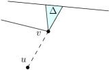
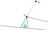
Sampling $C(S)$. Our goal is to obtain a random multiset $C^{\prime\prime}(S)\subseteq C(S)$ of size roughly $c(m/n)\log n$. To achieve this, we repeat the following procedure $4cn\log n$ times: We select two points $u$ and $v$ at random, with replacement, from the $2n$ endpoints of $S$. Note that there are $4n^{2}$ ways of doing this. Next, using $O(1)$ ray sweeping queries, we determine if $q$ is a vertex of some triangle $\Delta\in C(S)$ that has an edge collinear with $\overrightarrow{uv}$ and that lies to the left of $\overrightarrow{uv}$ (see Figure 11). Note that, for any $\Delta\in C(S)$, there is exactly one pair $(u,v)$ for which this is true. Therefore, if this test is affirmative then $\Delta$ is an element drawn uniformly at random from $C(S)$ and we add it to our sample $C^{\prime\prime}(S)$. The probability that we increase the size of $C^{\prime\prime}(S)$ this way is $m_{S}/(4n^{2})$, where $m_{S}=|C(S)|=O(m)$.

Space, preprocessing time, and query time. To compute $C^{\prime\prime}(S)$ efficiently we use the ray-sweeping data structure described in the proof of Lemma 2. Each sampling step requires $O(1)$ ray-sweeping queries, which can be done in $O_{\epsilon}(n/\sqrt{\ell})$ time after $O_{\epsilon}(\ell)$ preprocessing. Thus, the expected time required to build the ray-sweeping data structure and perform $4cn\log n$ sampling steps is $O_{\epsilon}(\ell+(cn\log n)(n/\sqrt{\ell})=O_{\epsilon}(\ell+cn^{2}/\sqrt{\ell})=O_{\epsilon}(c^{2/3}n^{4/3})$ for $\ell=c^{2/3}n^{4/3}$.

Each sampling step adds an element to $C^{\prime\prime}(S)$ with probability $m_{S}/(4n^{2})$. So, the number of samples in $C^{\prime\prime}(S)$ is a binomial random variable with parameters $4cn\log n$ and $m_{S}/(4n^{2})$ and the expected size of $C^{\prime\prime}(S)$ is therefore $c(m_{S}/n)\log n$. Using Chernoff’s Bounds, we find that the probability that the size of $C^{\prime\prime}(S)$ exceeds $ac(m_{S}/n)\log n$ is at most $n^{-\Omega(a)}$ for any $a>1$. This concentration result ensures that when building the data structure of Theorem 1 on the elements of $C^{\prime\prime}(S)$ the expected size, preprocessing time, and query time of the resulting structure are $O_{\epsilon}(k)$, $O_{\epsilon}(k)$, and $O_{\epsilon}((m/n)/\sqrt{k})$, respectively, for any $m/n\leq k\leq(m/n)^{2}$.

To summarize, for any $k$ with $m/n\leq k\leq(m/n)^{2}$, the above sampling procedure runs in $O_{\epsilon}(c^{2/3}n^{4/3}+k)$ expected time and produces a data structure of $O_{\epsilon}(k)$ expected size, that can answer queries in $O_{\epsilon}((m/n)/\sqrt{k})$ expected time. All that remains is to calibrate and check the accuracy of the results provided by the data structure.

Estimating $m^{\prime}_{p}$. Recall that our goal is to estimate $m^{\prime}_{p}$, the number of elements of $C(S)$ that contain the query point $p$, as $m^{\prime}_{p}$ is a 2-approximation to the number of segments of $S$ visible from $p$. Let

$$m^{\prime\prime}_{p}=(n/(c\log n))\cdot|\{\Delta\in C^{\prime\prime}(S):p\in\Delta\}|.\enspace.$$

(Note that computing $m^{\prime\prime}_{p}$ does not require knowing the value $m_{S}=|C(S)|$.) Each step of the sampling procedure finds an element $\Delta\in C(S)$ such that $p\in\Delta$ with probability exactly $m^{\prime}_{p}/(4n^{2})$. Since the sampling procedure runs for $4cn\log n$ steps, this implies that the number of triangles in $C^{\prime\prime}(S)$ that contain $p$ is a binomial random variable with parameters $4cn\log n$ and $m^{\prime}_{p}/(4n^{2})$. Therefore,

$$\mathrm{E}[m^{\prime\prime}_{p}]=(n/(c\log n))(4cn\log n)(m^{\prime}_{p}/4n^{2})=m^{\prime}_{p}\enspace.$$

That is, $m^{\prime\prime}_{p}$ is an unbiased estimator of $m^{\prime}_{p}$. Furthermore, applying Chernoff’s bounds to the underlying binomial random variable (see Appendix B), we find that

$$\Pr\{|m^{\prime\prime}_{p}-m^{\prime}_{p}|\geq\delta n\}\leq n^{-\Omega(\delta^{2}cn/m_{p})}$$

for any $\delta>0$. Combining this with (2) we obtain

$$\Pr\{m_{p}-\delta n\leq m^{\prime\prime}_{p}\leq 2m_{p}+\delta n\}\geq 1-n^{-\Omega(\delta^{2}cn/m_{p})}\enspace.$$

This establishes the accuracy of the data structure and completes the proof of our last theorem:

Theorem 4.

Let $S$ be a set of $n$ disjoint line segments whose visibility graph has $m$ edges and let $c>1$ and $0<\alpha<1$ be real valued parameters. There exists a data structure $D$ that can approximate the number of segments of $S$ visible from any query point $p$ such that:

1. $D$ has expected size $O_{\epsilon}((cm/n)^{1+\alpha})=O_{\epsilon}((cn)^{1+\alpha)})$,

2. $D$ can be constructed in time $O_{\epsilon}(c^{2/3}n^{4/3}+(cn)^{1+\alpha})$,

3. $D$ can perform a query in $O_{\epsilon}((cm/n)^{(1/2)(1-\alpha)})=O_{\epsilon}((cn)^{(1/2)(1-\alpha)})$ time, and

4. for any $\delta>0$, when querying $D$ with a point $p$ that sees $m_{p}$ points of $S$, $D$ returns a value $m^{\prime\prime}_{p}$ that satisfies $m_{p}-\delta n\leq m^{\prime\prime}_{p}\leq 2m_{p}+\delta n$ with probability at least $1-n^{-\Omega(\delta^{2}cn/m_{p})}$.

Example. Taking $c=dn^{1/3}$, for a large constant $d$, and $\alpha=0$, we get a data structure of size $O_{\epsilon}(n^{4/3})$ that can be constructed in time $O_{\epsilon}(n^{14/9})$ and that can, in $O_{\epsilon}(n^{2/3})$ time, effectively distinguish between viewpoints $p$ where $m_{p}\ll n^{2/3}$ and viewpoints $p$ where $m_{p}\gg n^{2/3}$.

4 Summary and Conclusions

Many open questions remain. The data structure for testing if a point is in $V_{S}(s)$ for a segment $S$ (Theorem 2) is near-optimal, at least assuming an $\Omega(n^{4/3})$ lower-bound for Hopcroft’s Problem. However, it is difficult to say if the data structures for approximate visibility counting are close to optimal. Our solutions reduce visibility counting to the problem of computing the depth of a query point in an arrangement of $O((m/n)\log n)$ (Theorem 3 and Theorem 4) or $O(m)$ () triangles. In both cases, it would be sufficient to give a relative approximation for the depth of the query point. Unfortunately, without some additional assumptions (such as fatness) about the triangles, there is currently no good solution to this problem.

The results in the current paper consider the problem of planar visibility counting, where $S$ is a set of disjoint line segments in $\mathbb{R}^{2}$. Of course, modern virtual environments are often 3-dimensional. Many of these environments are just barely 3-dimensional in the sense that they consist of a constant number of 2-dimensional layers that can be handled using the data structures presented in the current paper. However, ultimately we would like to develop data structures that store a set $S$ of disjoint triangles in $\mathbb{R}^{3}$ and can approximately count the number of elements of $S$ (at least partly) visible from a query point $p\in\mathbb{R}^{3}$.

Appendix

Appendix A Accuracy Bound for Theorem 3

In this appendix, we derive the error bound of the data structure of Theorem 3. To do this, we will use a version of Chernoff Bounds for binomial random variables [2, Appendix A.1] which states that, for a binomial random variable $B$ with mean $\mu$,

$$\Pr\{|B-\mu|\geq\tau\mu\}\leq\exp(-\Omega(\tau^{2}\mu))\enspace.$$ (3)

for any $\tau>0$.

Let $B$ be the number of samples in $S^{\prime\prime}$ visible from $p$, let $x=m^{\prime}_{p}$ be the number of segments in $S^{\prime}$ visible from $p$, and let $t=(c\log n)/n$. Then $B$ is a binomial$(x,t)$ random variable with expectation $\mu=xt$. We have that $|m^{\prime\prime}_{p}-m^{\prime}_{p}|\geq\delta n$ if and only if $|B-\mu|\geq t\delta n$. Taking $\tau=t\delta n/\mu$ and applying Equation (3) we obtain

$$\Pr\{|m^{\prime\prime}_{p}-m^{\prime}_{p}|\geq\delta n\} = \Pr\{|B-\mu|\geq t\delta n\}$$

$$\leq \exp(-\Omega(\left(t\delta n/\mu\right)^{2}\mu))$$

$$= \exp(-\Omega((t\delta n)^{2}/\mu))$$

$$= \exp(-\Omega((\delta n)^{2}t/x))$$

$$= \exp(-\Omega((\delta^{2}cn\log n)/x))$$

$$= n^{-\Omega(\delta^{2}cn/x))}$$

$$= n^{-\Omega(\delta^{2}cn/m^{\prime}_{p}))}$$

$$= n^{-\Omega(\delta^{2}cn/m_{p}))}\enspace,$$

as required.

Appendix B Accuracy Bound for Theorem 4

Let $B$ be the number of sample triangles in $C^{\prime\prime}(S)$ that contain $p$, let $x=m^{\prime}_{p}$ be the number of triangles in $C(S)$ that contain $p$, and let $t=x/(4n^{2})$. Then $B$ is a binomial$(4cn\log n,t)$ random variable with expected value $\mu=4tc\log n=(cx\log n)/n$.

We have that $|m^{\prime\prime}_{p}-m^{\prime}_{p}|\geq\delta n$ if and only if $|B-\mu|\geq\delta c\log n$. Taking $\tau=(\delta c\log n)/\mu$ and applying Equation (3) we obtain

$$\Pr\{|m^{\prime\prime}_{p}-m^{\prime}_{p}|\geq\delta n\} = \Pr\{|B-\mu|\geq\delta c\log n\}$$

$$= \exp(-\Omega(((\delta c\log n)/\mu)^{2}\mu))$$

$$= \exp(-\Omega((\delta c\log n)^{2}/\mu))$$

$$= \exp(-\Omega(\delta^{2}(cn\log n)/x))$$

$$= n^{-\Omega(\delta^{2}cn/x))}$$

$$= n^{-\Omega(\delta^{2}cn/m^{\prime}_{p}))}$$

$$= n^{-\Omega(\delta^{2}cn/m_{p}))}\enspace,$$

as required.

References

- [1] P. K. Agarwal and J. Erickson. Geometric range searching and its relatives. In B. Chazelle, J. E. Goodman, and R. Pollack, editors, Advances in Discrete and Computational Geometry, volume 223 of Contemporary Mathematics, pages 1–56. American Mathematical Society Press, 1999.
- [2] N. Alon and J. H. Spencer. The Probabilistic Method. John Wiley & Sons, Hoboken, third edition, 2008.
- [3] B. Aronov, L. J. Guibas, M. Teichmann, and L. Zhang. Visibility queries and maintenance in simple polygons. Discrete & Computational Geometry, 27(4):461–483, 2002.
- [4] T. Asano. An efficient algorithm for finding the visibility polygon for a polygonal region with holes. IEICE Transactions, E68-E:557–589, 1985.
- [5] P. Bose, A. Lubiw, and J. I. Munro. Efficient visibility queries in simple polygons. Computational Geometry Theory and Applications, 23(3):313–335, 2002.
- [6] T. M. Chan. Geometric applications of a randomized optimization technique. Discrete & Computational Geometry, 22(4):547–567, 1999.
- [7] M. de Berg, O. Cheong, M. van Kreveld, and M. Overmars. Computational Geometry Algorithms and Applications. Springer, third edition, 2008.
- [8] J. Erickson. New lower bounds for Hopcroft’s problem. Discrete & Computational Geometry, 16(4):389–418, 1996.
- [9] J. Erickson. Lower bounds for linear satisfiability problems. Chicago Journal of Theoretical Computer Science, 1999, 1999.
- [10] M. Fischer, M. Hilbig, C. Jähn, F. Meyer auf der Heide, and M. Ziegler. Planar visibility counting. CoRR, abs/0810.0052, 2008.
- [11] M. Fischer, M. Hilbig, C. Jähn, F. Meyer auf der Heide, and M. Ziegler. Planar visibility counting. In Proceedings of the 25th European Workshop on Computational Geometry (EuroCG 2009), pages 203–206, 2009.
- [12] S. K. Ghosh and D. Mount. An output sensitive algorithm for computing visibility graphs. SIAM Journal on Computing, 20:888–910, 1991.
- [13] L. J. Guibas, R. Motwani, and P. Raghavan. The robot localization problem. SIAM Journal on Computing, 26(4):1120–1138, 1997.
- [14] J. Matoušek. Efficient partition trees. Discrete & Computational Geometry, 8:315–334, 1992.
- [15] J. Matoušek. Lectures on Discrete Geometry, volume 212 of Springer Graduate Texts in Mathematic. Springer, 2002.
- [16] J. O’Rourke. Art Gallery Theorems and Applications. Oxford University Press, 1987.
- [17] M. Pocchiola and G. Vegter. The visibility complex. International Journal of Computational Geometry and Applications, 6(3):279–308, 1996.
- [18] S. Suri and J. O’Rourke. Worst-case optimal algorithms for constructing visibility polygons with holes. In Proceedings of the Second Annual Symposium on Computational Geometry (SCG 84), pages 14–23, 1984.
- [19] A. Zarei and M Ghodsi. Efficient computation of query point visibility in polygons with holes. In Proceedings of the 21st Annual ACM Symposium on Computational Geometry (SCG 2005), 2005.