Fluctuation-induced collective motion: A single-particle density analysis

Abstract

In a system of noisy self-propelled particles with interactions that favor directional alignment, collective motion will appear if the density of particles increases beyond a certain threshold. In this paper, we argue that such a threshold may depend also on the profiles of the perturbation in the particle directions. Specifically, we perform mean-field, linear stability, perturbative and numerical analyses on an approximated form of the Fokker-Planck equation describing the system. We find that if an angular perturbation to an initially homogeneous system is large in magnitude and highly localized in space, it will be amplified and thus serves as an indication of the onset of collective motion. Our results also demonstrate that high particle speed promotes collective motion.

I Introduction

The interesting phenomena of flocking in animals Couzin et al. (2005); Buhl et al. (2006); Sumpter (2006) and self-organized patterns in motile cells Tsimring et al. (1995); Riedel et al. (2005); Budrene and Berg (1991) are currently driving the intense theoretical study of collective motion among self-propelled particles Vicsek et al. (1995); Toner and Tu (1995, 1998); Gregoire_PRL04 ; Dossetti et al. (2009); Romanczuk et al. (2009); Aldana et al. (2007); D’Orsogna et al. (2006); Kruse et al. (2004); Bertin et al. (2006); Peruani et al. (2008). In particular, a comprehensive linear stability analysis on the onset of collective motion from the perspective of Boltzmann equation has recently appeared Bertin et al. (2009). Models for collective motion usually involve motile particles that possess alignment interactions and angular noise. Collective motion is then observed if the density of particles increases beyond a certain threshold. Besides density fluctuations, fluctuations in the heading directions of the particles constitute another important aspect of the system. Here, we study a minimal model for collective motion and show that the threshold for collective motion transition may depend on the profiles of directional fluctuations. Specifically, we find that an initial directional perturbation to a spatially homogeneous system will be amplified, if the perturbation is large in magnitude and is highly localized in space. We also demonstrate that high particle speed promotes collective motion.

To achieve our results, we first write down the Fokker-Planck equation describing the single-particle density distribution of the system in Sect. II. We then investigate in Sect. III the equation in the Fourier space of the directional component, and argue that only the lower order modes are important at the onset of collective motion. As a result, the dynamics of the distribution function can be captured by a set of three nonlinear coupled differential equations, which we subsequently study with linear stability analysis in Sect. IV. In Sect. V, we go beyond the linear stability regime by investigating the dynamical equations perturbatively and numerically.

II Model

In this work, we follow Peruani et al. (2008) and consider a minimal model for collective motion in two dimensions, where every particle is assumed to have constant speed and that their interactions consist only of directional alignment mechanism. Noise is incorporated in the direction of travel. Specifically, let there be $N$ particles in a volume of $V$, their equations of motion are:

$$\frac{{\rm d}\mathbf{r}_{i}}{{\rm d}t} = \frac{2u}{\pi}\mathbf{v}(\theta_{i})$$ (1)

$$\frac{{\rm d}\theta_{i}}{{\rm d}t} = -\frac{\partial U}{\partial\theta_{i}}(\mathbf{R},\Theta)+\sqrt{2D}\eta_{i}(t)$$ (2)

where $1\leq i\leq N$, $\mathbf{R}\equiv(\mathbf{r}_{1},\ldots,\mathbf{r}_{N})$, $\Theta\equiv(\theta_{1},\ldots,\theta_{N})$, $\mathbf{v}(\theta)\equiv(\cos\theta,\sin\theta)$, and the noise is assumed to be Gaussian characterized by the following moments:

$$\langle\eta_{i}(t)\rangle=0\ \ \ ,\ \ \ \langle\eta_{i}(t)\eta_{j}(t^{\prime})\rangle=\delta_{ij}\delta(t-t^{\prime})$$ (3)

Moreover, the alignment interaction is assumed to be of very short range and thus can be approximated by a delta function:

$$U(\mathbf{R},\Theta)=-\frac{g}{\pi}\sum_{i<j}\delta^{(2)}(\mathbf{r}_{i}-\mathbf{r}_{j})\cos(\theta_{i}-\theta_{j})\ .$$ (4)

If we denote the probability distribution of the density of particles in the state $(\mathbf{R},\Theta)$ at time $t$ by $f(t,\mathbf{R},\Theta)$, then the Fokker-Planck equation corresponding to the system is Zwanzig (2001):

$$\frac{\partial f}{\partial t} = \sum_{i}\bigg{\{}D\frac{\partial^{2}}{\partial\theta_{i}^{2}}f-\frac{2u}{\pi}\nabla_{\mathbf{r}_{i}}\cdot[\mathbf{v}(\theta_{i})f]\bigg{\}}$$ (5)

$$+\frac{g}{\pi}\sum_{i<j}\frac{\partial}{\partial\theta_{i}}\left[\delta^{(2)}(\mathbf{r}_{i}-\mathbf{r}_{j})\sin(\theta_{i}-\theta_{j})f\right]\ .$$

Naturally, we are not interested in all the information captured by $f$, and we will from now on focus on the single-particle density function, $\rho$,

$$\rho(\mathbf{r}_{1},\theta_{1})=\frac{(N!)\int{\rm d}r_{2}\cdots{\rm d}r_{N}{\rm d}\theta_{2}\cdots{\rm d}\theta_{N}f(\mathbf{R},\Theta)}{(N-1)!}\ .$$

From Eq. (5), we can express $\rho$ in terms of the two-particle density function $\rho^{(2)}$:

$$\frac{\partial\rho(\mathbf{r},\theta)}{\partial t}=D\frac{\partial^{2}\rho(\mathbf{r},\theta)}{\partial\theta^{2}}-\frac{2u}{\pi}\left[\cos\theta\frac{\partial\rho(\mathbf{r},\theta)}{\partial x}+\sin\theta\frac{\partial\rho(\mathbf{r},\theta)}{\partial y}\right]$$

$$+\frac{g}{\pi}\frac{\partial}{\partial\theta}\bigg{[}\int{\rm d}\theta^{\prime}\int{\rm d}r^{\prime}\delta^{(2)}(\mathbf{r}-\mathbf{r}^{\prime})\sin(\theta-\theta^{\prime})\rho^{(2)}(\mathbf{r},\theta,\mathbf{r}^{\prime},\theta^{\prime})\bigg{]}\ .$$ (6)

where

$$\rho^{(2)}(\mathbf{r}_{1},\theta_{1},\mathbf{r}_{2},\theta_{2})=\frac{(N!)\int{\rm d}r_{3}\cdots{\rm d}r_{N}{\rm d}\theta_{3}\cdots{\rm d}\theta_{N}f(\mathbf{R},\Theta)}{(N-2)!}\ .$$

The above manipulation is akin to the BBGKY hierarchy formalism Huang (1987). To continue with our analytical treatment, we will ignore the second ordered correlation and adopt the product distribution assumption: $\rho^{(2)}(\mathbf{r},\theta,\mathbf{r}^{\prime},\theta^{\prime})=\rho(\mathbf{r},\theta)\rho(\mathbf{r}^{\prime},\theta^{\prime})$. This assumption is similar to the molecular chaos assumption in the context of Boltzmann equation, and is also adopted in Bertin et al. (2006, 2009).

By Fourier transforming the above equation with respect to the angular variable, $\theta$, we have:

$$\partial_{t}\hat{\rho}_{n}(\mathbf{r}) = -Dn^{2}\hat{\rho}_{n}(\mathbf{r})-u\Big{[}\partial_{x}\big{(}\hat{\rho}_{n+1}(\mathbf{r})+\hat{\rho}_{n-1}(\mathbf{r})\big{)}$$ (7)

$$+{\rm i}\partial_{y}\big{(}\hat{\rho}_{n-1}(\mathbf{r})-\hat{\rho}_{n+1}(\mathbf{r})\big{)}\Big{]}$$

$$-gn\Big{[}\hat{\rho}_{-1}(\mathbf{r})\hat{\rho}_{n+1}(\mathbf{r})-\hat{\rho}_{1}(\mathbf{r})\hat{\rho}_{n-1}(\mathbf{r})\Big{]}$$

where $\rho(\mathbf{r},\theta)=\sum_{n=-\infty}^{\infty}\hat{\rho}_{n}(\mathbf{r}){\rm e}^{-{\rm i}n\theta}$.

Since $\hat{\rho}_{n}(\mathbf{r})$ are complex, we will denote them by $a_{n}(\mathbf{r})+{\rm i}b_{n}(\mathbf{r})$ where $a_{n}$ and $b_{n}$ are real functions. In relation to the original density function, we have

$$\rho(\mathbf{r},\theta) = \sum_{n\in{\bf Z}}[a_{n}(\mathbf{r})+{\rm i}b_{n}(\mathbf{r})]{\rm e}^{-{\rm i}n\theta}$$

$$= a_{0}(\mathbf{r})+2\sum_{n>1}\Big{[}a_{n}(\mathbf{r})\cos(n\theta)+b_{n}(\mathbf{r})\sin(n\theta)\Big{]}$$

where for the second equality, the following conditions for the $a_{n}$ and $b_{n}$ have been employed:

$$a_{n}=a_{-n}\ \ \ ,\ \ \ b_{n}=-b_{-n}\ ,$$ (9)

which are due the fact that $\rho$ is real. Writing Eq. 7 in terms of the $a_{n}$ and $b_{n}$, we have for $n\in{\bf Z}$,

$$\partial_{t}a_{n} = -Dn^{2}a_{n}-u\Big{[}\partial_{x}(a_{n+1}+a_{n-1})-\partial_{y}(b_{n-1}-b_{n+1})\Big{]}-gn\Big{[}a_{1}(a_{n+1}-a_{n-1})+b_{1}(b_{n-1}+b_{n+1})\Big{]}$$ (10)

$$\partial_{t}b_{n} = -Dn^{2}b_{n}-u\Big{[}\partial_{x}(b_{n+1}+b_{n-1})+\partial_{y}(a_{n+1}-a_{n-1})\Big{]}-gn\Big{[}a_{1}(b_{n+1}-b_{n-1})-b_{1}(a_{n+1}+a_{n-1})\Big{]}\ .$$ (11)

Note that the arguments $(t,\mathbf{r})$ in $a_{n}$ and $b_{n}$ are omitted in the above equations to ease notation.

III Mean-field approximation

To avoid having to deal with the above infinite set of differential equations, we will sort to truncate the number of differential equations to be considered. To do so, we first study the system in a mean-field manner MFref , i.e., we set $\hat{\rho}_{n}(t,\mathbf{r})=\hat{\rho}_{n}(t)$ for all $\mathbf{r}$. Eqs (10) and (11) then become

$$\frac{{\rm d}a_{n}}{{\rm d}t} = -Dn^{2}a_{n}-gn\Big{[}a_{1}(a_{n+1}-a_{n-1})$$ (12)

$$+b_{1}(b_{n-1}+b_{n+1})\Big{]}$$

$$\frac{{\rm d}b_{n}}{{\rm d}t} = -Dn^{2}b_{n}-gn\Big{[}a_{1}(b_{n+1}-b_{n-1})$$ (13)

$$-b_{1}(a_{n+1}+a_{n-1})\Big{]}\ .$$

Note that ${\rm d}a_{0}/{\rm d}t=0$ due to the fact that $a_{0}$ corresponds to the overall density of the system, which does not change.

Let us assume that the $b$ modes are not excited at $t=0$ and so we need only focus on the $a$ modes. By inspecting Eq. II, we see that the omission of the $b$ modes is the same as focusing only on angular perturbation of the form $\cos(\theta)$, i.e., the particles are more likely to be heading in the positive $x$ direction. With this simplification, the first three modes are of the form:

$$\frac{{\rm d}a_{1}}{{\rm d}t} = ga_{0}a_{1}-(Da_{1}+ga_{1}a_{2})$$ (14)

$$\frac{{\rm d}a_{2}}{{\rm d}t} = 2ga_{1}^{2}-(4Da_{2}+ga_{1}a_{3})$$ (15)

$$\frac{{\rm d}a_{3}}{{\rm d}t} = 3ga_{1}a_{2}-(9Da_{3}+ga_{1}a_{4})\ .$$ (16)

At the onset of collective motion (CM) from a spatially and angularly homogeneous system, we expect that $|a_{n}|\ll 1$ for $n>1$. Let us define $\epsilon$ as $\max_{n>1}|a_{n}|$ at the onset of CM, we see that only ${\rm d}a_{1}/{\rm d}t$ is of order $\epsilon$ while all the time-derivatives for the higher order modes are of order $\epsilon^{2}$. Furthermore, the coefficients associated with the damping term $D$ for the $n-$th modes scale with $n^{2}$, which further suggests that only the lower order modes are important. Another corroborating evidence is from Bertin et al. (2006, 2009) where the authors employed their scaling ansatz, which is supported by their numerical simulations, to argue that the higher order modes are indeed negligible at the onset of CM. Based on all these reasons, we will truncate the original dynamical equations, Eq. (7), by omitting all $\hat{\rho}_{n}$ for $n>2$. Focusing again only on the $a$ modes, we have

$$\frac{{\rm d}a_{0}}{{\rm d}t} = 0$$ (17)

$$\frac{{\rm d}a_{1}}{{\rm d}t} = (-D+ga_{0}-ga_{2})a_{1}$$ (18)

$$\frac{{\rm d}a_{2}}{{\rm d}t} = -4Da_{2}+2ga_{1}^{2}\ .$$ (19)

A simple fixed point analysis on the above equations indicate that the existence of non-zero fixed point for $a_{1}$ and $a_{2}$ is only possible when

$$ga_{0}-D>0\ .$$ (20)

This condition has previously been derived in Peruani et al. (2008). Expectedly, the above condition indicates that collective motion is facilitated by having strong interaction ($g$), high particle density ($a_{0}$) and weak noise ($D$).

IV Linear stability analysis

We now continue with our truncation approximation, but with the spatial variable re-installed into Eqs (12) and (13). Before we start to analyze the set of differential equations, we note that by inspecting Eqs (10) and (11), we see that the $a_{n\geq 1}$ and $b_{n\geq 1}$ modes are coupled exclusively to different spatial dimensions – the $x$ and $y$ dimensions respectively. In other words, if the system is initially homogeneous in the $x$ dimension, then the $x$ dimension will remain homogeneous, and vice versa. We will therefore, as in the previous section, assume that the $b$ modes are not excited and focus only on the $a$ modes. With this simplification, we arrive at the following dynamical equations:

$$\partial_{t}\alpha = -2u\partial_{x}\beta$$ (21)

$$\partial_{t}\beta = -D\beta-u\partial_{x}(\alpha+\gamma)+g\beta(\alpha-\gamma)$$ (22)

$$\partial_{t}\gamma = -4D\gamma-u\partial_{x}\beta+2g\beta^{2}\ ,$$ (23)

where we have used the Greek letters $\alpha$, $\beta$ and $\gamma$ to denote $a_{0}$, $a_{1}$ and $a_{2}$ respectively.

The fixed point in the homogeneous phase corresponds to $\alpha=1$, $\beta=0$ and $\gamma=0$ where we have set the unit length in such a way that the density of the particles is one. We now perform linear stability analysis on this fixed-point by considering the linear response of the system to a small perturbation of the form:

$$\alpha = 1+A{\rm e}^{\lambda t+{\rm i}qy}$$ (24)

$$\beta = B{\rm e}^{\lambda t+{\rm i}qy}$$ (25)

$$\gamma = C{\rm e}^{\lambda t+{\rm i}qy}$$ (26)

where $A,B,C\ll 1$ and $q$ is an arbitrary frequency. Substituting the above into Eqs (21) and (22) gives the following condition on $\lambda$:

$$\frac{\lambda(\lambda+D-g)(\lambda+4D)}{3\lambda+8D}=-u^{2}q^{2}\ ,$$ (27)

which indicates that $\lambda>0$ if and only if $g>D$. In other words, we have recovered the condition found in our previous mean-field analysis (c.f. Eq. (20)).

Although this result is consistent with what we found in the previous section, pieces of the picture at the onset of CM are still lacking. For instance, the phase transition condition found here does not depend on the speed of the particle $u$. This is unsatisfactory because we know that long range order would not be possible if $u=0$ Toner and Tu (1995, 1998). Moreover, it is desirable to see how the coupling between the spatial and temporal dimension affects the rise of the excited mode $\beta$. To gain insight in these questions, we will go beyond the linear stability regime and analyse the dynamical equations with perturbative method in the next section.

Figure 1: The density profiles of $\alpha$, $\beta$ and $\gamma$ at different times obtained by numerically solving the set of differential equations in Eqs (28) to (30), with the following parameters: $u=1/\sqrt{3}$, and $D=g=\xi=\sigma=0.1$.

V Beyond linear stability analysis

In this section, we will study Eqs (21) to (23) perturbatively. Specifically, we will assume that $D,g\ll 1$, in the units of distance and time set by having $\alpha(t=0,x)=1$ and $u=1/\sqrt{3}$. Physically, these assumptions amount to limiting our discussion to the regime where the particles’ angular fluctuations and interaction strength are small. Furthermore, since we are primarily interested in the dynamics at the onset of CM, we will assume that $g/D$ is of order unity (c.f. Eq. (20)). These assumptions allow us to employ $D$ (or equivalently, $g$) as the expansion parameter in our perturbative treatment. In contrast to the linear stability analysis in the previous section where the perturbation magnitude is assumed to be small enough that the nonlinear term is negligible, the perturbative approach adopted here allows us to study the effects of the nonlinear term on the dynamics.

In the aforementioned units, Eqs (21) to (23) are:

$$\partial_{t}\alpha = -\frac{2}{\sqrt{3}}\partial_{x}\beta$$ (28)

$$\partial_{t}\beta = -D\beta-\frac{1}{\sqrt{3}}\partial_{x}(\alpha+\gamma)+g\beta(\alpha-\gamma)$$ (29)

$$\partial_{t}\gamma = -4D\gamma-\frac{1}{\sqrt{3}}\partial_{x}\beta+2g\beta^{2}\ .$$ (30)

We now expand $\alpha$ as:

$$\alpha=\alpha_{0}+D\alpha_{1}+{\cal O}(D^{2})\ ,$$ (31)

and similarly for $\beta$ and $\gamma$. The zero-th order (in $D$) terms follow the following differential equations:

$$\partial_{t}\alpha_{0} = -\frac{2}{\sqrt{3}}\partial_{x}\beta_{0}$$ (32)

$$\partial_{t}\beta_{0} = -\frac{1}{\sqrt{3}}\partial_{x}(\alpha_{0}+\gamma_{0})$$ (33)

$$\partial_{t}\gamma_{0} = -\frac{1}{\sqrt{3}}\partial_{x}\beta_{0}\ .$$ (34)

The above set of differential equations can be solved by employing the Laplace-Fourier Transform method. For the initial conditions of $\alpha_{0}(t=0,x)=1$, $\beta_{0}(t=0,x)=\xi{\rm e}^{-y^{2}/(2\sigma^{2})}/\sqrt{2\pi}\sigma$ and $\gamma_{0}(t=0,x)=0$. The solutions are:

$$\alpha_{0} = 1+\frac{\xi}{\sqrt{6\pi}\sigma}\bigg{[}U^{-}-U^{+}\bigg{]}$$ (35)

$$\beta_{0} = \frac{\xi}{2\sqrt{2\pi}\sigma}\bigg{[}U^{-}+U^{+}\bigg{]}$$ (36)

$$\gamma_{0} = \frac{\xi}{2\sqrt{6\pi}\sigma}\bigg{[}U^{-}-U^{+}\bigg{]}\ ,$$ (37)

where

$$U^{\pm}=\exp\left(-\frac{(x\pm t)^{2}}{2\sigma^{2}}\right)\ .$$ (38)

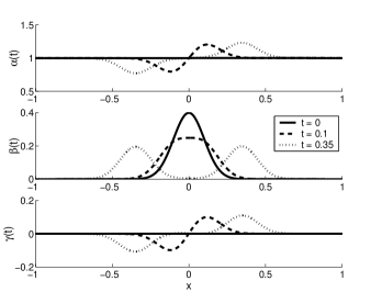
In other words, a Gaussian perturbation in $\beta$ at $t=0$ splits into two Gaussian distributions traveling in opposite directions with unit speed (as a result of setting $u$ to $1/\sqrt{3}$). The perturbation also induces in $\alpha$ and $\gamma$ two solitary waves in the form a Gaussian distribution traveling with unit speed in the positive direction, and an inverted Gaussian density wave traveling in the opposite direction (c.f. Fig. 1). This is akin to the stripe traveling wave pattern found in the CM phase Gregoire_PRL04 ; Bertin et al. (2009).

The differential equations governing the first-order terms are:

$$\partial_{t}\alpha_{1} = -\frac{2}{\sqrt{3}}\partial_{x}\beta_{1}$$ (39)

$$\partial_{t}\beta_{1} = -\beta_{0}-\frac{1}{\sqrt{3}}\partial_{x}(\alpha_{1}+\gamma_{1})+\frac{g}{D}\beta_{0}(\alpha_{0}-\gamma_{0})$$ (40)

$$\partial_{t}\gamma_{1} = -4\gamma_{0}-\frac{1}{\sqrt{3}}\partial_{x}\beta_{1}+\frac{2g}{D}\beta^{2}_{0}\ .$$ (41)

where $\alpha_{0}$, $\beta_{0}$ and $\gamma_{0}$ above are now given by Eqs (35) to (37). The initial conditions for the above equations are: $\alpha_{1}(t=0,x)=\beta_{1}(t=0,x)=\gamma_{1}(t=0,x)=0$.

Figure 2: The temporal evolutions of (a) $A$ (c.f. Eq. (43)) and (b) $B$ (c.f. Eq. (43)), obtained by numerically solving the set of differential equations in Eqs (28) and (30), with $D=g=\xi=0.1$. (c) The zoom-in plot of $B(t)$ at small time with the three curves corresponding to the theoretical expressions given in Eq. (47).

Figure 3: The temporal evolutions of (a) $A$ (c.f. Eq. (43)) and (b) $B$ (c.f. Eq. (43)), obtained by numerically solving the set of differential equations in Eqs (28) and (30), with $g=b=\sigma=0.1$. The zoom-in plot of $B(t)$ at small time with the three curves corresponding to the theoretical expressions given in Eq. (47).

Before we attempt to study the above set of differential equations, let us look for some meaningful quantities that quantifies the effect of the initial perturbation. For instance, the temporal evolution of total increase in $\beta_{1}$ due to the initial perturbation can be obtained from Eq. (40):

$$\partial_{t}\left(\int_{-\infty}^{\infty}{\rm d}y\beta_{1}(t,y)\right) = \int_{-\infty}^{\infty}{\rm d}y\left(\frac{g}{D}\alpha-1\right)\beta$$ (42)

$$= \xi\left(\frac{g}{D}-1\right)$$

This indicates that when summed over the whole space, the $\beta$ mode is amplified only if $g>D$. This is again consistent with the result we obtained in Sect. III and Sect.  IV.

Besides the above quantity, the following two quantities are also of interest:

$$A(t)\equiv\int_{0}^{\infty}{\rm d}x\alpha(t,x)\ ;\ B(t)\equiv\int_{0}^{\infty}{\rm d}x\big{[}\beta(t,x)-\beta(0,x)\big{]}\ .$$ (43)

Namely, $A$ and $B$ correspond to the responses in the density ($\alpha$) and in the $\beta$ mode in the direction of the angular perturbation. These are in fact arguably better quantities to consider as they capture the directional nature of the perturbation. From Eq. (40), we have:

$$\frac{{\rm d}B(t)}{{\rm d}t} = \frac{\xi(g-D)}{2}+\frac{g\xi^{2}}{8\sqrt{3\pi}\sigma}{\rm erf}\left(\frac{t}{\sigma}\right)$$ (45)

$$+\frac{D}{\sqrt{3}}[\alpha_{1}(t,x=0)+\gamma_{1}(t,x=0)]\ .$$

In the appendix, we demonstrate that

$$\alpha_{1}(t,y=0)+\gamma_{1}(t,y=0)=\frac{g\xi^{2}}{\pi\sigma^{2}}t+{\cal O}(t^{3})\ .$$ (46)

In other words, up to order ${\cal O}(t^{3})$, we have

$$B(t)=\frac{b(g-D)t}{2}+\frac{5gt^{2}}{8\sqrt{3}\pi}\left(\frac{\xi}{\sigma}\right)^{2}\ .$$ (47)

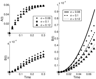
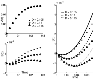
The third term in the right hand side above highlights the importance of the term $\xi/\sigma$, especially when $D\simeq g$. Fig. 2(a) and (b) display the temporal evolutions of $A(t)$ and $B(t)$ by solving Eqs (28) and (29) numerically in the case of $D=g$. They clearly show the amplification of the initial perturbation, which we have taken as an indication for the onset of collective motion in longer time. Fig. 2(c) demonstrates that at short time, the dynamics is well described by the expression in Eq. (47). Furthermore, due to the positive second term in the R.H.S. above, the formula for $B(t)$ suggests that there is a possibility of perturbation amplification even if $D>g$, e.g., when $\xi/\sigma\gg 1$. This is indeed shown to be the case in Fig. 3(a) and (b), where amplification of the perturbation is seen for $D/g\sim 1.1$. In other words, a sharp perturbation in the angular domain is able to induce collective motion even if the density is below the phase transition threshold as obtained in the mean-field model.

If we now restore the speed, $u$, and the initial density, $c$, where $c=\alpha(t=0,x)$, into Eq. (47), we have

$$B(t)=\frac{bc(cg-D)t}{2}+\frac{5guct^{2}}{8\pi}\left(\frac{\xi}{\sigma}\right)^{2}\ .$$ (48)

Note that the speed of the particles only appears in the second term above, which is positive. Hence, the above formula suggests that the particle speed has a net effect of amplifying the initial perturbation and thus facilitating collective motion transition.

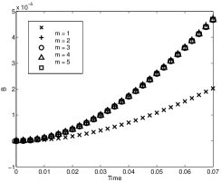
As a verification on the validity of our approximation adopted in our analytical calculations, we numerically simulate Eqs (10) and (11) with higher order modes included and find that there are no discernible differences for the parameter range investigated in this work (c.f. Fig. 4).

Figure 4: The evolution of $B(t)$ obtained by numerical simulating the differential equations Eqs (10) and (11) with the initial condition discussed in Sect. V. The parameters are $g=D=\xi=\sigma=0.1$. In the simulations, only the 0-th to the $m$-th $a$ modes are included. In other words, we assume that $a_{n>m}=0$ and $b_{n\in{\bf Z}}=0$.

VI Conclusion

In summary, starting with a Fokker-Planck equation for a minimal model of CM, we derived a set of three coupled differential equations that describes the system at the onset of CM. We then studied the equations with mean-field, linear stability, perturbative and numerical analyses, and found that if an angular perturbation is large in magnitude and highly localized in space, it will be amplified and thus serves as an indication of the onset of collective motion. Our calculations also demonstrate the importance of particle speed for collection motion transition. As a result, it is indicative that the critical point for CM may depend on the speed $u$, the perturbation magnitude $b$ and the perturbation wavelength $\sigma$. This is in contrast to the mean-field and linear stability analyses where only the hydrodynamic, or infinite-wavelength, mode dictates the onset of CM. Our results therefore highlights the importance of incorporating the nonlinear term into the analysis.

The main limitation of this work is on the approximation adopted – the omissions of higher order modes. While we believe that such an approximation is appropriate at the onset of CM, it would be highly desirable to have a systematic method to incorporate the higher order modes into the dynamics. Besides the consideration of the higher order modes, singular perturbation method would also be needed to investigate the long-time behaviour of the system footnote . We believe that these aspects would constitute two promising directions for future investigation.

*

Appendix A

We are unable to solve the set of differential equations shown in Eqs (39) to (41) analytically. But since only the leading orders in $x$ and $t$ are of interests, we will replace the $U^{\pm}$ in $\alpha_{0},\beta_{0},\gamma_{0}$ (c.f. Eqs (35) to (37)) by

$$\tilde{U}^{\pm}\equiv 1-\frac{(x\pm t)^{2}}{2\sigma^{2}}+\left[\frac{(x\pm t)^{2}}{2\sigma^{2}}\right]^{2}\ .$$ (49)

With this simplification, the differential equations can be solved by the Laplace-Fourier Transform method and the relevant results are:

$$\alpha_{1}(t,y=0)={\cal O}(t^{3})\ \ \ ,\ \ \ \gamma_{1}(t,y=0)=\frac{g\xi^{2}}{\pi\sigma^{2}}t+{\cal O}(t^{3})\ .$$ (50)

References

- Couzin et al. (2005) I. D. Couzin, J. Krause, N. R. Franks, and S. A. Levin, Nature 433, 513 (2005).
- Buhl et al. (2006) J. Buhl, D. J. T. Sumpter, I. D. Couzin, J. J. Hale, E. Despland, E. R. Miller, and S. J. Simpson, Science 312, 1402 (2006).
- Sumpter (2006) D. J. T. Sumpter, Philosophical Transactions of the Royal Society B: Biological Sciences 361, 5 (2006).
- Tsimring et al. (1995) L. Tsimring, H. Levine, I. Aranson, E. B. Jacob, I. Cohen, O. Shochet, and W. N. Reynolds, Physical Review Letters 75, 1859 (1995).
- Riedel et al. (2005) I. H. Riedel, K. Kruse, and J. Howard, Science 309, 300 (2005).
- Budrene and Berg (1991) E. O. Budrene and H. C. Berg, Nature 349, 630 (1991).
- Vicsek et al. (1995) T. Vicsek, A. Czirók, E. B. Jacob, I. Cohen, and O. Shochet, Physical Review Letters 75, 1226 (1995).
- Toner and Tu (1995) J. Toner and Y. Tu, Physical Review Letters 75, 4326 (1995).
- Toner and Tu (1998) J. Toner and Y. Tu, Physical Review E 58, 4828 (1998).
- (10) G. Grégoire and H. Chaté, Physical Review Letters 92, 025702 (2004)
- Dossetti et al. (2009) V. Dossetti, F. J. Sevilla, and V. M. Kenkre, Physical Review E (Statistical, Nonlinear, and Soft Matter Physics) 79, 051115 (2009).
- Romanczuk et al. (2009) P. Romanczuk, I. D. Couzin, and L. S. Geier, Physical Review Letters 102, 010602 (2009).
- Aldana et al. (2007) M. Aldana, V. Dossetti, C. Huepe, V. M. Kenkre, and H. Larralde, Physical Review Letters 98, 095702 (2007).
- Kruse et al. (2004) K. Kruse, J. F. Joanny, F. Jülicher, J. Prost, and K. Sekimoto, Physical Review Letters 92, 078101 (2004).
- Bertin et al. (2006) E. Bertin, M. Droz, and G. Grégoire, Physical Review E (Statistical, Nonlinear, and Soft Matter Physics) 74, 022101 (2006).
- Peruani et al. (2008) F. Peruani, A. Deutsch, and M. Bär, The European Physical Journal - Special Topics 157, 111 (2008).
- D’Orsogna et al. (2006) M. R. D’Orsogna, Y. L. Chuang, A. L. Bertozzi, and L. S. Chayes, Physical Review Letters 96, 104302 (2006).
- Bertin et al. (2009) E. Bertin, M. Droz, and G. Gregoire, Journal of Physics A: Mathematical and Theoretical 42, 445001 (2009).
- Zwanzig (2001) R. Zwanzig, Nonequilibrium Statistical Mechanics (Oxford University Press, Oxford, 2001).
- Huang (1987) K. Huang, Statistical Mechanics (Wiley, 1987), 2nd ed.
- (21) Please also see M. Aldana and C. Huepe, J. Stat. Phys. 112, 135 (2003), and W. Ebeling, Physica A 314, 92 (2002) and the references therein for other relevant mean-field results.
- (22) See, e.g., C. M. Bender and S. A. Orszag, Advanced Mathematical Methods for Scientists and Engineers: Asymptotic Methods and Perturbation Theory (Springer, 1999).