Automorphic properties of low energy string amplitudes in various dimensions

Abstract:

This paper explores the moduli-dependent coefficients of higher derivative interactions that appear in the low-energy expansion of the four-supergraviton amplitude of maximally supersymmetric string theory compactified on a $d$-torus. These automorphic functions are determined for terms up to order $\partial^{6}\mathcal{R}^{4}$ and various values of $d$ by imposing a variety of consistency conditions. They satisfy Laplace eigenvalue equations with or without source terms, whose solutions are given in terms of Eisenstein series, or more general automorphic functions, for certain parabolic subgroups of the relevant U-duality groups. The ultraviolet divergences of the corresponding supergravity field theory limits are encoded in various logarithms, although the string theory expressions are finite. This analysis includes intriguing representations of $SL(d)$ and $SO(d,d)$ Eisenstein series in terms of toroidally compactified one and two-loop string and supergravity amplitudes.

1 Introduction

In this paper we will pursue a programme of elucidating exact properties of the four-supergraviton scattering amplitude in the low energy expansion of string theory compactified from $10$ to $D=10-d$ dimensions on a $d$-torus, ${\mathcal{T}}^{d}$. Although this is a very small corner of M-theory it is one in which precise statements can be made. In particular, the combination of maximal supersymmetry and U-duality is very constraining [2]. The low energy expansion of the scattering amplitude in $D$-dimensional space-time has the general form

$$A_{D}(s,t,u)=A_{D}^{analytic}(s,t,u)+A_{D}^{nonan}(s,t,u)\,,$$ (1.1)

where we have separated analytic and nonanalytic functions of the Mandelstam invariants, $s$, $t$ and $u$ ($s=-(k_{1}+k_{2})^{2}$, $t=-(k_{1}+k_{4})^{2}$, $u=-(k_{1}+k_{3})^{2}$ and $s+t+u=0$). Although it is not obvious that such a separation can be made in a useful manner to all orders in the low energy expansion, it is sensible and useful at the orders to be considered in this paper. The analytic part of the amplitude has the expansion (in the Einstein frame)

$$A_{D}^{analytic}=\mathcal{E}^{(D)}_{(0,-1)}({\mathcal{M}}_{K\backslash G})\,{\mathcal{R}^{4}\over\sigma_{3}}+\sum_{p=0}^{\infty}\sum_{q=0}^{\infty}\mathcal{E}^{(D)}_{(p,q)}({\mathcal{M}}_{K\backslash G})\,\sigma_{2}^{p}\,\sigma_{3}^{q}\,\mathcal{R}^{4}\,,$$ (1.2)

which is the general symmetric polynomial in the Mandelstam invariants, which enter in the dimensionless combinations

$$\sigma_{n}=(s^{n}+t^{n}+u^{n})\,{\ell_{D}^{2n}\over 4^{n}}\,,$$ (1.3)

where $\ell_{D}$ is the Planck length in $D$ dimensions. The factor of $\mathcal{R}^{4}$ in (1.2) indicates the contraction of four powers of the Riemann curvature tensors linearised around flat space and contracted with a standard sixteen-index tensor, $t_{8}\,t_{8}$ [3]. The coefficient functions are necessarily automorphic functions that are invariant under the $D$-dimensional duality group, $G_{d}(\mathbb{Z})$, appropriate to compactification on a $d=(10-D)$-torus. These groups are listed in table 1. They are functions of the symmetric space, ${\mathcal{M}}_{K\backslash G}$, defined by the moduli, or the scalar fields, of the coset space $K\backslash G$. It is often convenient to express the analytic part of the amplitude in terms of a local one-particle irreducible effective action.

$D$	$G_{d}({\mathbb{R}})=E_{d+1(d+1)}({\mathbb{R}})$	$K$	$G_{d}({\mathbb{Z}})$
10A	$GL(1,{\mathbb{R}})$	1	1
10B	$SL(2,{\mathbb{R}})$	$SO(2)$	$SL(2,{\mathbb{Z}})$
9	$GL(2,{\mathbb{R}})$	$SO(2)$	$SL(2,{\mathbb{Z}})$
8	$SL(3,{\mathbb{R}})\times SL(2,{\mathbb{R}})$	$SO(3)\times SO(2)$	$SL(3,{\mathbb{Z}})\times SL(2,{\mathbb{Z}})$
7	$SL(5,{\mathbb{R}})$	$SO(5)$	$SL(5,{\mathbb{Z}})$
6	$SO(5,5,{\mathbb{R}})$	$SO(5)\times SO(5)$	$SO(5,5,{\mathbb{Z}})$
5	$E_{6(6)}({\mathbb{R}})$	$USp(8)$	$E_{6(6)}({\mathbb{Z}})$
4	$E_{7(7)}({\mathbb{R}})$	$SU(8)/{\mathbb{Z}}_{2}$	$E_{7(7)}({\mathbb{Z}})$
3	$E_{8(8)}({\mathbb{R}})$	$SO(16)$	$E_{8(8)}({\mathbb{Z}})$

Table 1: The duality groups of maximal supergravity in $D=10-d\leq 10$ dimensions. The groups $G_{d}({\mathbb{R}})=E_{d(d)}({\mathbb{R}})$ are the real split forms of rank $d+1$ and $K$ are the maximal compact subgroups. In string theory these groups are broken to the discrete subgroups, $G_{d}({\mathbb{Z}})$ as indicated in the last column.

Although this paper will be concerned almost entirely with the analytic part of (1.1), $A^{analytic}$, it is important to consider its relationship to the nonanalytic part, $A^{nonan}$. This part of the amplitude contains the information about the massless thresholds that arise in perturbation theory and contribute to the nonlocal part of the effective action. Such contributions include the threshold structure of supergravity scattering amplitudes, and depend on the space-time dimension, $D$, in a sensitive manner. At sufficiently high values of $D$, a $L$-loop perturbative contribution in supergravity has ultraviolet divergences that are power-behaved in a momentum cut-off, $\Lambda$. Such divergences are absent in string theory and the dependence on a power of $\Lambda$ is replaced by a finite analytic term with a corresponding power of $\ell_{s}^{-1}$, where $\ell_{s}$ is the string length scale. As $D$ is decreased it reaches a critical value at which supergravity develops a logarithmic ultraviolet divergence. Introducing a momentum cutoff now produces a nonanalytic factor of the schematic form $A_{D}^{nonan}\sim\mathcal{R}^{4}\,s^{k}\,\log(-s/\Lambda^{2})$, which is replaced in string theory by

$$A_{D}^{nonan}\sim\mathcal{R}^{4}\,s^{k}\,\log(-\ell_{s}^{2}\,\mu\,s)\,,$$ (1.4)

where $\mu$ is a dimensionless scale, which is independent of the moduli and may be determined by a detailed string loop calculation. This expression is merely illustrative – the detailed dependence on the Mandelstam variables and pattern of logarithms is more complicated. For a discussion of such effects in the expansion of the genus-one contribution see [4]. Of course, there is some ambiguity in how such constant terms are assigned to the analytic and non-analytic pieces since $\mu$ may be changed to $\mu/\tilde{\mu}$ by adding $\mathcal{R}^{4}\,s^{k}\ \log\tilde{\mu}$ to the analytic term. In the subsequent discussions in this paper our convention will be to associate all such moduli-independent logarithms with the scale of non-analytic $s^{k}\,\log(-\ell_{s}^{2}\,\mu/\tilde{\mu}\,s)$ contributions to the amplitude. Furthermore, we will not discuss the precise values of the constant scales such as $\mu$, which can be determined by explicit string perturbation theory computations, such as that carried out at genus-one in [4]. As $D$ is decreased to values $D<D_{c}$, the nonanalytic terms are proportional to inverse powers of $s$, $t$ and $u$. For $D\leq 4$ the four-supergraviton amplitude possesses the standard infrared divergences of a perturbative gravitational theory, which will not be discussed here.

The first term in the expansion (1.2) ($p=0,q=-1$) has coefficient $\mathcal{E}^{(D)}_{(0,-1)}=3$ and is the classical supergravity tree-level term, with poles in $s$, $t$, $u$, and is determined by the Einstein–Hilbert action. This has trivial dependence on the moduli. The subsequent terms have a rich dependence on ${\mathcal{M}}$ that encodes both perturbative and non-perturbative information. This contrasts with supergravity, in which the continuous $G_{d}({\mathbb{R}})$ duality symmetry is unbroken, and amplitudes are independent of the moduli. The simplest non-trivial examples of automorphic functions arise in the ten-dimensional IIB theory, where the coset is $SO(2)\backslash SL(2)$, so there is a single complex modulus, $\Omega=\Omega_{1}+i\Omega_{2}$, and the duality group is $SL(2,\mathbb{Z})$. In this case the first two terms in the expansion beyond the classical term are given by particular examples of non-holomorphic Eisenstein series for $SL(2,\mathbb{Z})$

$${\bf E}_{s}(\Omega)=\sum_{(m,n)\neq(0,0)}\frac{\Omega_{2}^{s}}{|m+n\Omega|^{2s}}\,,$$ (1.5)

which satisfies the Laplace equation

$$\Delta_{\Omega}\,{\bf E}_{s}(\Omega)\equiv\Omega_{2}^{2}\,(\partial^{2}_{\Omega_{1}}+\partial^{2}_{\Omega_{2}})\,{\bf E}_{s}(\Omega)=s(s-1)\,{\bf E}_{s}(\Omega)\,,$$ (1.6)

and where $s$ is a (generally complex) index. Some important properties of these functions are reviewed in appendix B.3. The Fourier expansion of ${\bf E}_{s}$ in (B.38) has a zero mode or “constant term” that consists of the sum of two powers,

$$\int_{-\frac{1}{2}}^{\frac{1}{2}}d\Omega_{1}\,{\bf E}_{s}=2\zeta(2s)\Omega_{2}^{s}+2\sqrt{\pi}\,\frac{\Gamma(s-{\scriptstyle{1\over 2}})}{\Gamma(s)}\,\zeta(2s-1)\Omega_{2}^{1-s}\,,$$ (1.7)

which correspond to a tree-level and genus-$(s-1/2)$ contribution to the interaction in string perturbation theory. The non-zero modes correspond to exponentially suppressed $D$-instanton contributions to the interaction. The first term of this type is the lowest order term beyond the Einstein–Hilbert term, which is the $\mathcal{R}^{4}$ interaction for which $p=q=0$ and the coefficient is $\mathcal{E}^{(10)}_{(0,0)}(\Omega)={\bf E}_{{\scriptstyle{3\over 2}}}(\Omega)$ that has tree-level and one-loop perturbative contributions [5, 6]. The next term in (1.2), with $p=1,q=0$, corresponds to a $\partial^{4}\mathcal{R}^{4}$ interaction in the effective action, with a coefficient $\mathcal{E}^{(10)}_{(1,0)}(\Omega)=1/2\,{\bf E}_{{\scriptstyle{5\over 2}}}(\Omega)$ that has tree-level and two-loop contributions [7]. Both the $\mathcal{R}^{4}$ and $\partial^{4}\,\mathcal{R}^{4}$ interaction coefficients can be determined by imposing constraints implied by modified supersymmetry transformations that incorporate higher-derivative contributions [8, 9].

The next term has $p=0,q=1$ and corresponds to the $\partial^{6}\mathcal{R}^{4}$ interaction. Its coefficient $\mathcal{E}^{(10)}_{(0,1)}(\Omega)$ is not an Eisenstein series [10], but satisfies the interesting inhomogeneous Laplace eigenvalue equation,

$$(\Delta_{\Omega}-12)\,\mathcal{E}_{(0,1)}^{(10)}(\Omega)=-\left(\mathcal{E}^{(10)}_{(0,0)}(\Omega)\right)^{2}\,,$$ (1.8)

where the right-hand side is a source term proportional to the square of the coefficient of the $\mathcal{R}^{4}$ interaction. In this case the constant term has power-behaved terms corresponding to perturbative string theory contributions at genus $0,1,2,3$, as well as exponentially suppressed contributions corresponding to an infinite set of $D$-instanton – anti $D$-instanton pairs.

There is a certain amount of information about terms of order $\partial^{8}\,\mathcal{R}^{4}$ and higher, but these terms raise issues that go beyond the scope of this paper and will not be discussed here (see [1] for particular examples). Our main aim will be to extend the results up to order $\partial^{6}\mathcal{R}^{4}$ to the higher-rank duality groups that arise upon compactification to $D$ dimensions on a $d=(10-D)$-torus. There has been some work in this direction for the $\mathcal{R}^{4}$ term in [6, 10, 11] and for the $\partial^{4}\mathcal{R}^{4}$ and $\partial^{6}\mathcal{R}^{4}$ terms in [12, 13]. Here we will not only amend these and extend their scope, but more importantly, set it in the general framework of automorphic functions for higher-rank groups. Some of our ideas overlap with suggestions in [11, 14, 15] and related papers [16, 17], but they differ in important respects.

Our procedure, outlined in section 2, will be to constrain the expressions for the automorphic coefficient functions by requiring them to reproduce the correct expressions in three distinct degeneration limits:

(i) The decompactification limit from $D$ to $D+1$ dimensions. When the radius, $r_{d}$, of one compact dimension becomes large the part of the $D=(10-d)$-dimensional coefficient function, $\mathcal{E}^{(D)}_{(p,q)}$, that leads to a finite term in the $r_{d}\to\infty$ limit is required to reproduce the $(D+1)$-dimensional coefficient function, $\mathcal{E}^{(D+1)}_{(p,q)}$. In addition there are suppressed terms with powers of $r_{d}^{-n_{i}}$ (where the values of $n_{i}>0$ depend on $D$) multiplying $\mathcal{E}^{(D+1)}_{(p^{\prime},q^{\prime})}$, where $2p^{\prime}+3q^{\prime}<2p+3q$. There are also specific terms with positive powers of $s\,r^{2}_{d}$ that are necessary to account for the non-analytic thresholds in $D+1$ dimensions (see the discussion in [18] for more details). The remaining terms are exponentially suppressed in $r_{d}$ and will not be constrained in any direct fashion.

(ii) Perturbative string theory limit. In the limit in which the $D$-dimensional string coupling constant becomes small the expansion of $\mathcal{E}^{(D)}_{(p,q)}$ in powers of the $D$-dimensional string coupling, $y_{D}$, is required to reproduce the known perturbative string theory results. In order to make this comparison the contributions from genus-one string theory are derived in appendix D using the methods of [4]. Furthermore, the leading low energy contribution to $\partial^{4}\mathcal{R}^{4}$ from the genus-two string theory amplitude compactified on ${\mathcal{T}}^{2}$ is derived in appendix E.

(iii) The semi-classical M-theory limit. In the limit of decompactification to eleven-dimensional supergravity on ${\mathcal{T}}^{d+1}$ the part of the modular function that depends on the geometric moduli of the torus, which parameterise the coset space $SO(d+1)\backslash SL(d+1)$, should be reproduced. This will give the part of the coefficient function that transforms under $SL(d+1,{\mathbb{Z}})$. This is the limit in which the effects of wrapped $p$-branes are suppressed and the Feynman diagrams of compactified eleven-dimensional quantum supergravity should give a valid expansion in powers of the inverse volume of the torus, ${\mathcal{V}}_{d+1}$  [6, 7, 10, 1]. The analysis of one-loop and two-loop expressions is reviewed in appendix G.

As we will emphasize, our analysis of these three limits makes contact with properties of the “constant terms” of the generalised Eisenstein series associated with various parabolic subgroups of the U-duality groups [19]. This viewpoint indicates the extent of the very powerful symmetries that relate these three limits for any value of $n$. Furthermore it gives a unified view of the relation between the theory in different dimensions by considering a nested set of (maximal) parabolic subgroups 

$$E_{8(8)}\supset E_{7(7)}\dots\supset E_{1(1)}=SL(2)\,,$$ (1.9)

where the sequence corresponds to successive decompactifications, as outlined in point (i) above. We are here using the usual economic notation for the duality groups in Table 1 in which $G_{d}=E_{d+1(d+1)}$ refers to the real split form of the classical group of rank $d+1$ (and so is related to the coset for string theory compactified on a $d$-torus).

In other words, we will use the explicit properties of string/M-theory in higher dimensions to constrain the particular automorphic functions that arise as coefficients in lower dimensions. We will therefore be focussing on very special cases of the general Eisenstein series. We will see that these particular cases have many interesting properties.

This analysis of the coefficients in various dimensions is somewhat complicated, as well as repetitive, so the casual reader could choose to skip the details in the bulk of the paper and read the brief summary in section 6.

The main arguments will begin in section 3, where we will describe the results for the $\mathcal{R}^{4}$ interaction. The explicit $\mathcal{E}^{(D)}_{(0,0)}$ coefficients in dimensions $D\geq 6$ will be obtained in terms of Eisenstein series that satisfy Laplace eigenvalue equations on moduli space space, building on the work of [6, 10, 11, 15] . The $D=8$ case is of interest because it contains the logarithmic dependence that encodes the one-loop logarithmic ultraviolet divergence of maximal supergravity. The fact that string theory is finite is manifested by the cancellation of an apparent divergence, subject to suitable regularisation. This arises because $\mathcal{E}^{(8)}_{(0,0)}$ is the sum of two Eisenstein series that each have poles in the parameter $s$ at appropriate values of $s$. A suitable analytic continuation leads to a cancellation of the poles in these two terms, leaving a logarithmic dependence on a modulus that can be identified with the logarithm that arises in the low energy supergravity limit. Formally these considerations extend to lower dimensions $D\geq 3$, in which the duality groups are those in the $E_{d+1(d+1)}$ sequence, where $d=10-D$. In all cases these series are finite, despite apparent poles, which cancel leaving crucial logarithmic dependence on moduli that are also expected for a consistent string theory interpretation.

In section 4 this analysis will be extended to the $\partial^{4}\mathcal{R}^{4}$ interaction, for which the coefficients are $\mathcal{E}^{(D)}_{(1,0)}$. Building on the analyses in [10, 12] we will first discuss the $D=9,8$ cases. The $D=7$ expression will then be analyzed. This is particularly interesting since it reproduces the two-loop logarithm characteristic of the ultraviolet divergence of maximal supergravity [22]. In order to satisfy the conditions (i)-(iii) we are led to a specific combination of two Eisenstein series for $SL(5)$. As before, the precise combination of Eisenstein series is one for which the divergent pole terms cancel, reflecting the absence of ultraviolet divergences in string theory. The analysis of the $D=6$ case with duality group $SO(5,5)$ will be left for the discussion in section 6, since our analysis is incomplete. In this case we make strong use of results for constant terms of Eisenstein series by Stephen Miller and is not as complete. There is no obvious obstacle to the extension to $D<6$ higher-rank duality groups, although this will not be discussed in this paper.

Section 5 concerns the $\partial^{6}\mathcal{R}^{4}$ interaction in $D=9$, $8$ and $7$ dimensions. To some extent the $D=8,9$ cases overlap with the analysis in [13], demonstrating how the Laplace equation with a source term generalizes for the larger duality groups. In each case the source term is the square of the $\mathcal{R}^{4}$ coefficient, $\mathcal{E}^{(D)}_{(0,0)}$. In $D=8$ this source possesses both $\log$ and $(\log)^{2}$ terms that are required for the solution to have requisite interpretation in the low energy limit of string theory. For example, maximal supergravity has a two-loop logarithmic ultraviolet divergence multiplying $\partial^{6}\mathcal{R}^{4}$, as well as a logarithmic contribution from the one-loop $D=8$ counterterm, which are reproduced by our modular coefficients.

Section 6 will summarize our results and describe some issues relating to the extension to higher-rank groups and higher derivative interactions. In particular, we will summarise in a compact manner the set of homogeneous and inhomogeneous Laplace eigenvalue equations satisfied by the coefficient functions for values of $D$ discussed in this paper, but which we argue should be valid in any dimension in the range $3\leq D\leq 10$. We will also make comments about the form of certain coefficients in $D\leq 6$ dimensions.

Technical details are given in several appendices.

2 Degeneration limits and Eisenstein series for parabolic subgroups

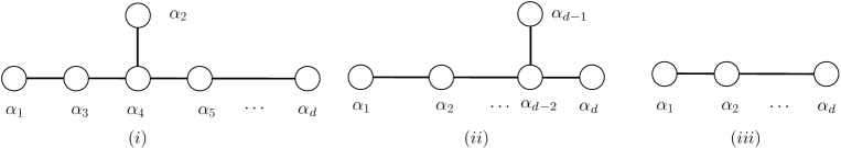
Figure 1: The Dynkin diagrams relevant to: (i) the $E_{d(d)}$ ($d\leq 8$) type II duality groups of type II string theory compactified to $D=11-d$ dimensions on a $(d-1)$-torus. Successive decompactifications to higher dimensions are obtained by deleting the nodes $\alpha_{d},\alpha_{d-1}\ \dots$ in (i); (ii) The T-duality groups $SO(10-D,10-D)$ obtained by deleting the left node $\alpha_{1}$ of (i) are the symmetries of string perturbation theory in $D$ dimensions; (iii) The $SL(11-D)$ groups obtained by deleting node $\alpha_{2}$ in (i) are associated with the geometric compactification of eleven-dimensional supergravity on a $(11-D)$-torus.

The duality groups of maximally supersymmetric closed-string theory are associated with the series of Dynkin diagrams in figure 1(i) that may be obtained from the $E_{8(8)}$ diagram by deleting the right nodes in a sequential manner. This generates the diagrams for the $E_{d(d)}$ series. In terms of string theory compactified on a $d$-torus, ${\mathcal{T}}^{d}$, the deletion of a right node labelled $\alpha_{d+1}$ corresponds to the decompactification of a radius, $r_{d}\to\infty$ ($d\geq 2$). This is the degeneration limit (i) of the previous section. The limit of small string coupling, or string perturbation theory, corresponds to deleting the left node labelled $\alpha_{1}$. This is the degeneration limit (ii) and gives a series of terms with symmetry $SO(d,d)$ (where the right node is again $\alpha_{d+1}$). The ${\mathcal{T}}^{d}$ compactification of string theory may be viewed as the ${\mathcal{T}}^{d+1}$ compactification of eleven-dimensional M-theory. The limit (iii) is one in which the M-theory volume of ${\mathcal{T}}^{d+1}$ becomes large, ${\mathcal{V}}_{d+1}\to\infty$, in which semiclassical eleven-dimensional geometry is a good approximation and the duality symmetry reduces to $SL(d)$. This is the degeneration limit in which the node $\alpha_{2}$ in figure 1(i) is deleted.

2.1 Parabolic subgroups

Parabolic sub-algebras of a semisimple Lie Algebra $\mathfrak{g}=\textrm{Lie}(G)$ with $\mathfrak{h}$ a Cartan sub-algebra are defined as follows [23, 24]. If $\Delta$ is the set of simple roots (a basis of roots) and $R^{+}$ the set of positive roots spanned by $\Delta$. Then $\mathfrak{b}=\mathfrak{h}+\oplus_{\alpha\in R^{+}}\,\mathfrak{g}_{\alpha}$, where $\mathfrak{g}_{\alpha}$ is the root space associated with the root $\alpha$, is the associated Borel sub-algebra. Consider a partition of the positive root space $\Delta$ into disjoint sets $\Delta_{1}$ and $\Delta_{2}$ so $\Delta=\Delta_{1}\sqcup\Delta_{2}$. We define, $R_{1}$ the set of positive roots spanned by $\Delta_{1}$ and $R_{2}$ the set of positive roots spanned by $\Delta_{2}$. Define

$$\mathfrak{p}_{\Delta_{2}}=\mathfrak{h}+\bigoplus_{\alpha\in R^{+}\cup(-R_{1})}\mathfrak{g}_{\alpha},\qquad\mathfrak{l}_{\Delta_{2}}=\mathfrak{h}+\bigoplus_{\alpha\in R_{1}\cup(-R_{1})}\mathfrak{g}_{\alpha},\qquad\mathfrak{n}_{\Delta_{2}}=\bigoplus_{\alpha\in R_{2}}\mathfrak{g}_{\alpha},$$ (2.1)

This defines the parabolic sub-algebra $\mathfrak{p}_{\Delta_{2}}$ associated with the set of positive roots $R_{1}$, $\mathfrak{l}_{\Delta_{2}}$ is its Levi factor and $\mathfrak{n}_{\Delta_{2}}$ the unipotent radical. Clearly if $\Delta_{2}\subset\hat{\Delta}_{2}$ then $\mathfrak{p}_{\hat{\Delta}_{2}}\subset\mathfrak{p}_{\Delta_{2}}$.

$\bullet$ When $\mathfrak{p}_{\Delta}=\mathfrak{b}$, $R_{2}$ is the set of all the positive roots (and $R_{1}=\emptyset$) the associated parabolic is the minimal parabolic sub-algebra.

$\bullet$ When $\mathfrak{p}_{\emptyset}=\mathfrak{g}$ (equivalently when $R_{2}=\emptyset$), $R_{1}$ is the set of all the positive roots the associated parabolic sub-algebra is the Lie Algebra $\mathfrak{g}$.

$\bullet$ Maximal parabolic sub-algebras different from $\mathfrak{g}$ are defined by singling out one simple root $\alpha_{i}$ and taking $\Delta_{2}=\{\alpha_{i}\}$. We denote the maximal parabolic sub-group by $P_{\alpha_{i}}$, with ${\rm rank}\ P_{\alpha_{i}}={\rm rank}(G)-1$.

$\bullet$ The (standard) parabolic subgroup of $GL(n)$ is defined as the group of matrices of the form, for $n=n_{1}+\cdots+n_{q}$,

$$P(n_{1},\dots,n_{q})=\begin{pmatrix}U_{1}&*&*\\ 0&\ddots&*\\ 0&0&U_{q}\end{pmatrix},\qquad\textrm{where~{}}U_{i}\in GL(n_{i})\,,$$ (2.2)

which can be factored in the form

$$P(n_{1},\dots,n_{q})=L(n_{1},\dots,n_{q})\,N(n_{1},\dots,n_{q})\,.$$ (2.3)

Here

$$N(n_{1},\dots,n_{q})=\begin{pmatrix}I_{n_{1}}&*&*\\ 0&\ddots&*\\ 0&0&I_{n_{q}}\end{pmatrix}\,\qquad\textrm{where~{}}I_{n}=\textrm{diag}(1,\dots,1)$$ (2.4)

is the unipotent radical and

$$L(n_{1},\dots,n_{q})=\begin{pmatrix}U_{1}&0&0\\ 0&\ddots&0\\ 0&0&U_{q}\end{pmatrix}\,,$$ (2.5)

is the Levi component. The minimal parabolic subgroup is given by $P(1,\dots,1)$. A given maximal parabolic subgroup has a characteristic pattern of zeroes in the upper off-diagonal elements of $N$. For example, the $SL(3,{\mathbb{R}})$ maximal parabolic subgroup [25],

$$P(1,2)=\begin{pmatrix}*&*&*\\ 0&*&*\\ 0&*&*\end{pmatrix}$$ (2.6)

has a unipotent radical of the form

$$N(1,2)=\begin{pmatrix}1&\nu_{1}&\nu_{2}\\ 0&1&0\\ 0&0&1\end{pmatrix}\,,$$ (2.7)

where $\nu_{1}$ and $\nu_{2}$ are real angular variables.

Three cases will be of particular interest in this paper. These concern the maximal parabolic subgroups given in the table 2, which are obtained by deleting the left node, the right node and the upper node of the Dynkin diagrams shown in fig. 1.

deleted node	$E_{8}$	$E_{7}$	$E_{6}$	$E_{5}=D_{5}$	$E_{4}=A_{4}$	$E_{3}=A_{2}A_{1}$
left	$D_{7}$	$D_{6}$	$D_{5}$	$D_{4}$	$D_{3}$	$D_{2}$
upper	$A_{7}$	$A_{6}$	$A_{5}$	$A_{4}$	$A_{3}$	$A_{2}$
right	$E_{7}$	$E_{6}$	$D_{5}$	$A_{4}$	$A_{2}A_{1}$	$A_{1}A_{1}$

Table 2: Maximal Parabolic subgroups of $E_{d(d)}$ arising in string theory are of the form $GL(1)\times X_{d-1}$, where the rank-$(d-1)$ subgroups are listed. We use the notation $A_{d}=SL(d+1)$, $D_{d}=SO(d,d)$. Each parabolic subgroup can be decomposed as the product $P_{\alpha}=N_{\alpha}L_{\alpha}$ of a unipotent radical $N_{\alpha}$ and a Levi factor $L_{\alpha}$. The Levi factors determine the Lie groups generated by the remaining nodes of the Dynkin diagram, which are listed in the table.

There are several interesting coincidences.

• In $D=7$, where the U-duality group is $E_{4(4)}=SL(5)$, the symmetry group of string perturbation theory is $SL(4)=SO(3,3)$, which is also the symmetry of M-theory on ${\mathcal{T}}^{4}$ in the decompactification to eleven dimensions.

• $E_{5(5)}=SO(5,5)$ arises in the $D=6$ theory, for which the group $SL(5)$ arises both as the symmetry of M-theory on $\mathcal{T}^{5}$ limit and as the U-duality group upon decompactification to $D=7$.

• $SO(5,5)$ arises both as the symmetry of string perturbation theory in the $D=5$ theory and as the decompactification limit to the $D=5$ theory, which has duality group $E_{5(5)}$.

• $E_{6(6)}$ arises as the U-duality group in $D=5$ and is symmetric under the interchange of nodes $1$ and $6$. This symmetry interchanges the limit of decompactification to $D=6$ with the perturbative string theory limit.

2.2 Eisenstein series for maximal parabolic subgroups and their constant terms.

The general Eisenstein series are automorphic functions of $d$ complex parameters, $s_{i}$ ($i=1,\dots,d$) associated with different parabolic subgroups of the $E_{d(d)}$ groups. Their definition may be found in [26, 19] and is briefly reviewed in appendix B. The construction of the minimal parabolic $SL(d)$ series, is also described in appendix B, based closely on notes by Stephen Miller and extensions of [25].

However, we are here primarily interested in very special cases corresponding to Eisenstein series for maximal parabolic subgroups, defined with respect to one particular node associated with the simple root $\alpha_{u}$. Such a series may be obtained by taking residues of the minimal parabolic series on the poles at $s_{i}=0$ for all $i$ except $i=u$, so the series depends on only one parameter, $s\equiv s_{u}$. The series can be indexed by the Dynkin label $[0^{u-1},1,0^{d-u}]$, where the $1$ is in the $u$’th position. The particular values of $u$ of interest to us will be determined on a case by case basis. Such a series for a maximal parabolic subgroup of the group $G$ will be denoted ${\bf E}^{G}_{[0^{u-1},1,0^{d-u}];s}$.

The simplest example is provided by the $SL(d)$ series with $u=1$ (the Epstein zeta function), which can be expressed as a sum over a single integer-valued $d$-component vector,

$${\bf E}^{SL(d)}_{[1,0^{d-2}];s}=\sum_{m^{i}\in\mathbb{Z}^{d}\backslash\{0\}}(m^{i}g_{ij}m^{j})^{-s}\,,$$ (2.8)

where the sum is over all values of $m^{i}$ with the value $m^{1}=m^{2}=\dots=0$ omitted. The metric $g_{ij}$ is the metric on $SO(d)\backslash SL(d)$. Our conventions for labelling the $SL(d)$ Dynkin diagrams are shown in figure 1(iii). A less trivial case that we will also need to consider is the $SL(d)$ Eisenstein series with $u=2$, which is given by

$${\bf E}^{SL(d)}_{[0,1,0^{d-3}];s}=\sum^{\prime}_{m^{i},n^{i}\in\mathbb{Z}^{d}}(m^{[i}n^{j]}g_{ik}g_{jl}m^{[k}n^{l]})^{-s}\,,$$ (2.9)

where $\sum^{\prime}$ here indicates the sum is over integers subject to the constraint that at least one minor $\delta^{[ij]}=m^{[i}n^{j]}$ is non-zero. For $SL(3)$ this series is proportional to the Epstein series, (2.8) with a shifted value of $s$, as we show in appendix B.4. More generally, the $SL(d)$ series ${\bf E}^{SL(d)}_{[0^{d-2},1];s}$ is proportional to the Epstein series with a shifted value of $s$, a simple consequence of the symmetry under $s\to d/2-s$, which follows from the Weyl symmetry of the weight lattice of $SL(d)$. Some relevant properties of the $SL(d)$ series are deduced in appendix B.

The other cases that will be considered explicitly in this paper are particular cases of Eisenstein series for $SO(d,d)$. In particular, these symmetries arise as T-duality groups of string perturbation theory in $10-d$ dimensions, and $SO(5,5)$ is the full U-duality group for $D=6$. We will discuss the maximal parabolic Eisenstein series of the form ${\bf E}^{SO(d,d)}_{[1,0^{d-1}];s}$, where the distinguished node is the one on the left in figure 1(ii) – i.e., associated with the vector representation. A number of properties of these series are obtained in appendix C based on a novel representation motivated by compactified two-loop Feynman diagrams. Although the series with more general Dynkin indices are relevant, we will not discuss them in this paper.

Constant terms.

The three degeneration limits (i), (ii) and (iii) that we are interested in correspond to decompositions of the Eisenstein series, ${\bf E}^{G}_{[0^{u-1},1,0^{d-u}];s}$, with respect to parabolic subgroups of the form, $P_{v}\equiv GL(1)\times G_{v}$, associated with one of three distinct nodes, $\alpha_{v}$, of the Dynkin diagram, as described earlier. The $GL(1)$ factor is parameterised by a real parameter $r$, which corresponds in limit (i) $(v=d)$ to the radius of the compact dimension, $r_{d}$, in limit (ii) ($v=1$) to the string coupling in $D$ dimensions, $y_{D}$, and in limit (iii) ($v=2$) to the volume of the M-theory torus, ${\mathcal{V}}_{11-D}$. In considering these limits we will retain all the terms that are power behaved in $r$. These are contained in the ‘constant terms’ obtained by taking the zero Fourier mode with respect to the components of the unipotent radical, $N_{v}$, associated with the parabolic subgroup $P_{\alpha_{v}}$ (defined in section 2.1). This is an integral over the entries, $\nu_{i}$, in the upper triangular matrix, $N_{v}$

$$A^{G}_{s}(u,v;g)=\int_{N_{v}/G(\mathbb{Z})\cap N_{v}}dn\,{\bf E}^{G}_{[0^{u-1},1,0^{d-u}];s}(gn)\,,$$ (2.10)

where $dn=\prod_{i}d\nu_{i}$ is the Haar measure on $N_{v}$. In order to avoid complicated notation, we will replace $\int_{N_{v}/G(\mathbb{Z})\cap N_{v}}dn$ by $\int_{P_{v}}$ so that

$$A^{G}_{s}(u,v;g)\equiv\int_{P_{v}}\,{\bf E}^{G}_{[0^{u-1},1,0^{d-u}];s}\,.$$ (2.11)

The angular integral (2.10) generalizes the $SL(2,{\mathbb{Z}})$ case of (1.7). The constant terms are expansions in powers of $r$ with coefficients that are Eisenstein series (or products of Eisenstein series, in the non-simple case) of the schematic form

$$A^{G}_{s}(u,v;g)=\sum_{i}c^{i}_{uv}\,r^{p_{i}}\,{\bf E}^{G_{v}}_{[\dots]_{i};s_{i}}\,,$$ (2.12)

where the values of the parameters $s_{i}$, $p_{i}$ depend on $u$ and $v$, and $r$ is a scale factor associated with the $GL(1)$ subgroup. This integration projects out the non-zero modes of the Eisenstein series, which are non-perturbative in $r$ and exponentially suppressed in the appropriate degeneration limit. The coefficients ${\cal E}^{(D)}_{(0,1)}$ of $\partial^{6}\mathcal{R}^{4}$ are not Eisenstein series and their constant terms do contain exponentially suppressed pieces corresponding to instanton—anti–instanton pairs.

The Eisenstein series for other maximal parabolic $SO(d,d)$ series, as well as those for the higher-rank $E_{d(d)}$ groups, are much more difficult to construct in terms of explicit sums over integers but their explicit properties can be obtained from their basic definition given in (B.1). Starting from that definition, the constant terms of their parabolic subgroups have been derived in [27], which is likely to be of use in developing these ideas further.

2.3 The expansion parameters.

In considering M-theory on a $(d+1)$-dimensional torus, ${\mathcal{T}}^{d+1}$, length scales are measured in units of the eleven-dimensional Planck length, $\ell_{11}$, whereas for string theory compactified on a $d$-dimension torus, ${\mathcal{T}}^{d}$, scales are measured in units of the string length, $\ell_{s}$, or the ten-dimensional Planck length scales of the IIA and IIB theories, $\ell_{10}^{A}$, $\ell_{10}^{B}$. These length scales are related by the well-known relations,

$$\ell_{11}=g_{A}^{1\over 3}\,\ell_{s}\,,\qquad\ell_{10}^{A}=g_{A}^{{1\over 4}}\,\ell_{s}\,,\qquad\ell_{10}^{B}=g_{B}^{{1\over 4}}\,\ell_{s}\,,\qquad R_{11}=g_{A}\,\ell_{s}\,,$$ (2.13)

where $g_{A}$ and $g_{B}$ are the type IIA and IIB coupling constants and $R_{11}$ is the radius of the extra M-theory circle.

Compactifying from $10$ to $D=10-d$ dimensions on ${\mathcal{T}}^{d}$ leads to the relations

$$\ell_{D}^{D-2}=y_{D}\,\ell_{s}^{D-2}\,,$$ (2.14)

where the quantity $y_{D}$ is defined by the $(10-d)$-dimensional T-duality invariant dilaton, which defines the $D$-dimensional coupling,

$$y_{10-d}\equiv e^{2\phi_{D}}=\frac{g_{A}^{2}\ell_{s}^{d}}{V^{A}_{d}}=\frac{g_{B}^{2}\ell_{s}^{d}}{V_{d}^{B}}\,,$$ (2.15)

where $V^{A}_{d}$ is the volume of the $d$-torus in IIA string units while $V^{B}_{d}$ is the volume in IIB units. Note further that he relation between the Planck length in $D$ dimensions and $D+1$ dimensions is

$$\ell_{D+1}^{D-1}=\ell_{D}^{D-2}\,\,r_{d}\,,$$ (2.16)

where $r_{d}$ is the radius of the $(d=10-D)$’th direction of ${\mathcal{T}}^{d}$ in IIB string units.

The parameters that we will use to define the three degeneration limits will be the following.

(i) The decompactification of a single dimension is given by the limit $r_{d}/\ell_{s}\to\infty$ in the string frame. We will be interested in expressing the result in the Einstein frame in $(D+1)$ dimensions at fixed coupling, in which case we will need to consider $r_{d}/\ell_{D+1}\to\infty$ with $y_{D+1}$ fixed. It will also be useful to introduce the U-duality invariant quantity defined in terms of the dimensionless volume of the string theory $d$-torus,

$$\nu_{d}^{-{\scriptstyle{1\over 2}}}=\frac{1}{\ell_{10}^{d}}V^{B}_{d}\,,$$ (2.17)

where we have set $\ell_{10}^{B}\equiv\ell_{10}$ in this and all subsequent expressions since we will not need to use $\ell_{10}^{A}$. It is easy to deduce the useful relations

$$\frac{r_{d}}{\ell_{D+1}}={r_{d}\over\ell_{s}}\,y_{D+1}^{-{1\over D-1}}=\nu_{d}^{-\frac{1}{2}}\,\nu_{d-1}^{D\over 2(D-1)}\,.$$ (2.18)

(ii) String perturbation theory is an expansion in powers of the $D$-dimensional string coupling, $e^{\phi^{B}_{D}}\equiv y_{D}^{1/2}$ when $y_{D}\to 0$.

(iii) Decompactification to semiclassical eleven-dimensional supergravity arises in the limit of large volume of the $(d+1)$-dimensional M-theory torus. This volume, ${\mathcal{V}}_{d+1}$, is defined by

$$G_{M\,IJ}=\mathcal{V}_{d+1}^{2\over d+1}\,\tilde{G}_{M\,IJ}\,,$$ (2.19)

where $G_{M\,IJ}$ ($I,J=1,\dots,d$) is the M-theory metric on ${\mathcal{T}}^{d+1}$ and $\tilde{G}_{IJ}$ has unit determinant. The dimensionless volume, $\hat{\mathcal{V}}_{d+1}$, can be expressed as

$$\hat{\mathcal{V}}_{d+1}\equiv\frac{1}{\ell_{11}^{d+1}}\mathcal{V}_{d+1}=\frac{1}{\ell_{11}^{d+1}}\sqrt{\det(G_{M\,IJ})}=g_{A}^{2-d\over 3}\,{V^{A}_{d}\over\ell_{s}^{d}}\,.$$ (2.20)

This can be converted to type-IIB units by compactifying one dimension of radius $r_{A}$ so that $V^{A}_{d}=r_{A}\times V_{d-1}$ and introducing the volume $V^{B}_{d}=r_{B}\times V_{d-1}$, where $r_{B}=\ell_{s}^{2}/r_{A}$, giving

$$\hat{\mathcal{V}}_{d+1}=g_{A}^{2-d\over 3}\,{V^{A}_{d}\over\ell_{s}^{d}}=g_{B}^{2-d\over 3}\,\left(r_{B}\over\ell_{s}\right)^{d-8\over 3}\,{V^{B}_{d}\over\ell_{s}^{d}}=\left(r_{B}\over\ell_{10}\right)^{d-8\over 3}\,{V^{B}_{d}\over\ell_{10}^{d}}\,.$$ (2.21)

The M-theory decompactification limit is given by the limit $\hat{\mathcal{V}}_{d+1}\to\infty$.

3 The $\mathcal{R}^{4}$ interaction

The first term in the low energy expansion of the maximally supersymmetric string theory amplitude beyond the tree-level term is the $\mathcal{R}^{4}$ term in (1.2), which is described by a term in the effective action of the form

$$S_{R^{4}}=\ell_{D}^{8-D}\,\int d^{D}x\,\sqrt{-G^{(10)}}\,{\cal E}^{(D)}_{(0,0)}\,\mathcal{R}^{4}\,.$$ (3.1)

In $D=10$ dimensions the coefficient function is given by [5]

$$\mathcal{E}^{(10)}_{(0,0)}(\Omega)={\bf E}^{SL(2)}_{[1];{\scriptstyle{3\over 2}}}(\Omega)\,,$$ (3.2)

which is the standard Eisenstein series for $SL(2,\mathbb{Z})$, that is conventionally denoted ${\bf E}_{{\scriptstyle{3\over 2}}}(\Omega)$ and satisfies the Laplace equation

$$\Delta^{(10)}\mathcal{E}^{(10)}_{(0,0)}={3\over 4}\,\mathcal{E}^{(10)}_{(0,0)}\,,$$ (3.3)

where $\Delta^{(10)}$ is the $SO(2)\backslash SL(2)$ Laplace operator,

$$\Delta^{(10)}\equiv\Omega_{2}^{2}\,(\partial^{2}_{\Omega_{1}}+\partial^{2}_{\Omega_{2}})\,.$$ (3.4)

The string frame expression for this interaction involves the identification

$${1\over\ell_{10}^{2}}\mathcal{E}^{(10)}_{(0,0)}(\Omega)={1\over\ell_{s}^{2}}\Omega_{2}^{{\scriptstyle{1\over 2}}}\,{\bf E}_{\frac{3}{2}}(\Omega)\,,$$ (3.5)

using the relation between the ten-dimensional Planck length and the string scale $\ell_{s}=\ell_{10}\,\Omega_{2}^{1/4}$. The perturbative expansion is associated with the constant term,

$${1\over\ell_{10}^{2}}\,\int_{-{\scriptstyle{1\over 2}}}^{\scriptstyle{1\over 2}}d\Omega_{1}\,{\cal E}^{(10)}_{(0,0)}(\Omega)=\frac{1}{\ell_{s}^{2}}\,\left(\frac{2\zeta(3)}{y_{10}}+4\zeta(2)\right)\,,$$ (3.6)

where $y_{10}=g_{B}^{2}$. This exhibits a tree-level term and a one-loop term.

We will here discuss the theory after compactification on ${\mathcal{T}}^{d}$ for $d=1,2,3,4$. In each case we will present a candidate expression and verify that it has the correct properties in the three degeneration limits described in section 1. Several aspects of this discussion reproduce earlier work, but our analysis will stress the framework that generalizes to other terms in the low energy expansion and to the larger U-duality groups.

3.1 Nine dimensions

The coefficient function in the nine-dimensional effective action ((3.1) with $D=9$) was determined in [5, 6] to be

$$\mathcal{E}_{(0,0)}^{(9)}=\nu_{1}^{-{3\over 7}}{\bf E}_{3\over 2}(\Omega)+4\zeta(2)\,\nu_{1}^{{4\over 7}}\,,$$ (3.7)

with $\nu_{1}=(r_{B}/\ell_{10})^{-2}$, which is invariant under the U-duality group $SL(2,\mathbb{Z})$. This coefficient function can straightforwardly be seen to satisfy the $SO(2)\backslash SL(2)\times{\mathbb{R}}^{+}$ Laplace eigenvalue equation,

$$\big{(}\Delta^{(9)}-{6\over 7}\big{)}\,\mathcal{E}^{(9)}_{(0,0)}=0\,,$$ (3.8)

where the Laplace operator for the nine-dimensional compactification has the form given in (H.6),

$$\Delta^{(9)}\equiv\Delta_{\Omega}+{7\over 4}\nu_{1}\partial_{\nu_{1}}(\nu_{1}\partial_{\nu_{1}})+{1\over 2}\nu_{1}\partial_{\nu_{1}}\,.$$ (3.9)

In order to see how the action behaves in various limits we write $\nu_{1}$ in terms of the other parameters as

$$\nu_{1}=\hat{\mathcal{V}}_{2}^{{\scriptstyle{3\over 2}}}\,,$$ (3.10)

or

$$\nu_{1}=\Omega_{2}^{-\frac{1}{2}}\,\left(\ell_{s}\over r_{B}\right)^{2}=y_{9}^{{\scriptstyle{1\over 4}}}\,\left(\frac{\ell_{s}}{r_{B}}\right)^{\frac{7}{4}}\,,$$ (3.11)

where $y_{9}=\ell_{s}/(\Omega_{2}^{2}\,r_{B})$, or

$$\nu_{1}=\left(\frac{\ell_{9}}{\ell_{10}}\right)^{14}=\left(\frac{r_{B}}{\ell_{10}}\right)^{-2}\,.$$ (3.12)

We will now review the manner in which the expression (3.7) reproduces the expected expressions in the three degeneration limits of interest.

(i) Decompactification to $D=10$

This limit is obtained by letting $r_{B}/\ell_{10}\to\infty$ in (3.7)

$${1\over\ell_{9}}\mathcal{E}^{(9)}_{(0,0)}={r_{B}\over\ell_{10}^{2}}\mathcal{E}^{(10)}_{(0,0)}+{4\zeta(2)\over r_{B}}\,.$$ (3.13)

The term proportional to $r_{B}$ survives the limit to give the $D=10$ expression (3.2).

(ii) $D=9$ perturbative string theory.

The perturbative expansion of (3.7) in the string frame is given by evaluating the constant term,

$${1\over\ell_{9}}\,\int_{-\frac{1}{2}}^{\frac{1}{2}}d\Omega_{1}\,\mathcal{E}^{(9)}_{(0,0)}={1\over\ell_{s}}\,\left({2\zeta(3)\over y_{9}}+4\zeta(2)\,\left({r\over\ell_{s}}+{\ell_{s}\over r}\right)\right)\,,$$ (3.14)

where $y_{9}=g_{B}^{2}\,\ell_{s}/r_{B}=g_{A}^{2}\,\ell_{s}/r_{A}$ is invariant under T-duality and $r=r_{B}$ or $r_{A}$ (where $r_{B}=\ell_{s}^{2}/r_{A}$). This expression is manifestly invariant under $r\to\ell_{s}^{2}/r$, as expected at this order in string perturbation theory. The coefficients are the same as those obtained directly from tree-level and one-loop string scattering amplitudes.

(iii) Semiclassical M-theory limit

The coefficient (3.7) is expressed in eleven-dimensional M-theory units by

$${1\over\ell_{9}}\,\mathcal{E}^{(9)}_{(0,0)}={1\over\ell_{11}}\,\left({\hat{\mathcal{V}}}_{2}^{-{1\over 2}}{\bf E}_{3\over 2}(\Omega)+4\zeta(2)\,{\hat{\mathcal{V}}}_{2}\right)\,.$$ (3.15)

This expression coincides with that obtained by evaluating the one-loop contribution of eleven-dimensional supergravity compactified on ${\mathcal{T}}^{2}$ [6]. This calculation has a $\Lambda^{3}$ divergent piece (where $\Lambda$ is a momentum cutoff) that is regularised by adding a counterterm, $c\,\mathcal{R}^{4}$, where the value of $c=4\zeta(2)$ is determined by imposing the equality of the IIA and IIB one-loop contributions [6]. Furthermore there are no higher-loop corrections to $\mathcal{R}^{4}$, so the result (3.7) is exactly given by the supergravity expression.

3.2 Eight dimensions

The effective action of the form (3.1) with $D=8$ was considered in [6, 10], based on evaluation of the contribution of one-loop eleven-dimensional supergravity compactified on ${\mathcal{T}}^{3}$. This takes into account the effect of super-supergravitons winding around the torus and has a manifest invariance under the modular group of the three-torus, $SL(3,\mathbb{Z})$. This was completed to the full duality group $E_{3(3)}=SL(3)\times SL(2)$ by extending the expression to include the effects of wrapped $M2$-branes, giving

$$\mathcal{E}^{(8)}_{(0,0)}={\hat{\bf E}}^{SL(3)}_{[10];{\scriptstyle{3\over 2}}}+2\hat{\bf E}^{SL(2)}_{[1];1}\,,$$ (3.16)

which is the form presented in [11]. The expressions ${\hat{\bf E}}^{SL(2)}_{[1];1}\equiv{\hat{\bf E}}_{1}$ and ${\hat{\bf E}}^{SL(3)}_{[10];{\scriptstyle{3\over 2}}}$ are regularised Eisenstein series (specifically, Epstein series) for the groups $SL(2)$ and $SL(3)$, respectively. Some properties of these series are discussed in appendix B and may be summarised as follows. The series ${\bf E}^{SL(2)}_{[1];s}={\bf E}_{s}$ and ${\bf E}^{SL(3)}_{[10];s}$ have poles at $s=1$ and $s=3/2$, respectively, which correspond to the presence of logarithmic singularities in the one-loop graviton scattering amplitude in $D=8$ dimensions – which may be expressed as poles in $\epsilon$ in dimensional regularisation, where $D=8+2\epsilon$. The hat  $\hat{}$  indicates that the pole part is subtracted, leaving only the finite part.

The Eisenstein series ${\bf E}^{SL(3)}_{[10];s}$ is a special case of the most general minimal parabolic Eisenstein series for $SL(3)$ and is discussed in (B.3). The general series has two parameters, $s_{1}$ and $s_{2}$, corresponding to the non-compact Cartan directions of the quotient $SO(3)\backslash SL(3)$, but the series of interest here has $s_{1}=s$, $s_{2}=0$. Appendix B.4 provides more details concerning this series, which is defined by (B.7) in the case $d=3$. The expression for the series ${\bf E}^{SL(3)}_{[10];s}$ in (B.49) is written with an explicit parameterisation of the metric in terms of the U-duality invariant mass for $D=8$ [11],

$${\bf E}^{SL(3)}_{[10];s}=\sum_{(m_{1},m_{2},m_{3})\in{\mathbb{Z}}^{3}\backslash\{0\}}\,\nu_{2}^{-{s\over 3}}\,\left({|m_{1}+m_{2}\Omega+Bm_{3}|^{2}\over\Omega_{2}}+{m_{3}^{2}\over\nu_{2}}\right)^{-s}\,.$$ (3.17)

The divergence at $s=3/2$ is regularised by setting $s=3/2+\epsilon$ and subtracting the pole (see appendix B.4 for details),

$${\bf E}^{SL(3)}_{[10];{3\over 2}+\epsilon}={2\pi\over\epsilon}+4\pi(\gamma_{E}-1)+{\hat{\bf E}}^{SL(3)}_{[10];\frac{3}{2}}+O(\epsilon)\,,$$ (3.18)

where the regularised series ${\hat{\bf E}}^{SL(3)}_{[10];\frac{3}{2}}$ is derived in (B.55) and is given by

$${\hat{\bf E}}^{SL(3)}_{[10];\frac{3}{2}}=\nu_{2}^{-{1\over 2}}\,{\bf E}_{3\over 2}(\Omega)+{4\pi\over 3}\,\log(\nu_{2})+O(e^{-\Omega_{2}^{\scriptstyle{1\over 2}}\,\nu_{2}^{-{\scriptstyle{1\over 2}}}},e^{-(\Omega_{2}\nu_{2})^{-{\scriptstyle{1\over 2}}}})\,.$$ (3.19)

In type IIB variables the $U$ modulus is acted only by the $SL(2)$ factor of the U-duality group $SL(3)\times SL(2)$. The $SL(2)$ Eisenstein series has a pole at $s=1$ as shown in (B.41),

$${\bf E}_{1+\epsilon}(U)={\pi\over\epsilon}-\pi\log(U_{2}|\eta(U)|^{4})+2\pi(\gamma_{E}-\log(2))+O(\epsilon)\,,$$ (3.20)

and the regularised series is obtained by subtracting the pole,

$$\hat{\bf E}_{1}(U)=-\pi\log(U_{2}|\eta(U)|^{4})\,.$$ (3.21)

So far we have discussed the singularities of the individual Eisenstein series ${\bf E}_{s}(U)$ and ${\bf E}^{SL(3)}_{[10];s}$. However the coefficient $\mathcal{E}^{(8)}_{(0,0)}$ (3.16) is a linear sum of these functions. A crucial factor (not discussed in past work) is that the singularities of the separate Eisenstein series should not be regularised independently. In fact, the singularities in (3.16) cancel each other when regularised in a manner consistent with the considerations that follow later later in this paper. This implies that (3.16) should be written as

$$\mathcal{E}^{(8)}_{(0,0)}=\lim_{\epsilon\to 0}\,\left({\bf E}^{SL(3)}_{[10];{\scriptstyle{3\over 2}}+\epsilon}+2{\bf E}^{SL(2)}_{[1];1-\epsilon}\right)-\log\mu_{(0,0)}\,,$$ (3.22)

where the hats have been removed since this expression is finite and $\log\mu_{(0,0)}=4\pi(2\gamma_{E}-1-\log(2))$ in order for (3.22) to agree with (3.16). We will later obtain this result from the decompactification limit for the coefficient of the $\mathcal{R}^{4}$ coefficient in $D=7$ dimensions, which is finite and reduces to (3.22) when $r_{3}\to\infty$ to give the $D=8$ expression. This is the first of several cases in which divergences in different contributions to a coefficient function cancel with a suitable regularsation.

The $SL(2)$ Eisenstein series at $s=1$ satisfies the Laplace equation (B.40)

$$\Delta_{SO(2)\backslash SL(2)}{\hat{\bf E}}^{SL(2)}_{[1];1}=\pi\,,$$ (3.23)

while the $SL(3)$ series satisfies

$$\Delta_{SO(3)\backslash SL(3)}\,{\hat{\bf E}}^{SL(3)}_{[10];{\scriptstyle{3\over 2}}}=4\pi\,,$$ (3.24)

where the $SO(3)\backslash SL(3)$ laplacian is given in (B.50). Therefore, applying the total $SO(3)\backslash SL(3)\times SO(2)\backslash SL(2)$ Laplacian of the eight-dimensional theory gives

$$\Delta^{(8)}\,\mathcal{E}^{(8)}_{(0,0)}=\Delta_{SO(3)\backslash SL(3)}{\hat{\bf E}}^{SL(3)}_{[10];{\scriptstyle{3\over 2}}}+2\,\Delta_{SO(2)\backslash SL(2)}{\hat{\bf E}}^{SL(2)}_{[1];1}=6\pi\ .$$ (3.25)

We will now verify that the expression (3.16) gives the correct expression in each of the three degeneration limits under consideration.

(i) Decompactification to $D=9$

The nine-dimensional limit is obtained by taking one of the radii of the two-torus to infinity, $r_{2}/\ell_{9}\to\infty$. This is seen by setting $T_{2}=r_{1}\,r_{2}/\ell_{s}^{2}$, $U_{2}=r_{2}/r_{1}$ and

$$\nu_{2}^{-1}=\Omega_{2}\,T_{2}^{2}=\nu_{1}^{-\frac{6}{7}}\,\left(r_{2}\over\ell_{9}\right)^{2}\,.$$ (3.26)

Using the expansions for ${\bf E}^{SL(3)}_{[10];s}$ in (B.4.1) and ${\bf E}_{s}(U)$ in (B.38), and the general definition of constant terms in (2.10), the constant term of the combination (3.16) in the $GL(1)\times SL(2)$ subgroup has the form

$$\int_{-\frac{1}{2}}^{\frac{1}{2}}dB_{\rm RR}dB_{\rm NS}\,\mathcal{E}^{(8)}_{(0,0)}={r_{2}\over\ell_{9}}\,\mathcal{E}^{(9)}_{(0,0)}-{14\pi\over 3}\,\log\left(\frac{r_{2}}{\ell_{9}\,\mu_{8}}\right)\,,$$ (3.27)

where the double integral is over the elements of the unipotent radical corresponding to this subgroup. At large $r_{2}$ and fixed $r_{1}$ the nonpertubative contributions are exponentially suppressed and only this constant term survives. The term proportional to $r_{2}$ gives the contribution to the $D=9$ action, in agreement with those in (3.7) with $r_{1}=r_{B}$. The $\log(r_{2}/\ell_{9})$ term in (3.27) is an important contribution to the massless threshold behaviour of the nonanalytic term in the one-loop four-supergraviton amplitude in eight dimensions, which has the form $\log(-\ell_{s}^{2}\,s)\,\mathcal{R}^{4}$. The $\log(r_{2}/\ell_{9})$ term in (3.27) combines with this contribution into $\log(-r_{2}^{2}s)\,\mathcal{R}^{4}$ which is part of the infinite series $(r_{2}^{2}\,s)^{k}\,\log(-r_{2}^{2}s)\,\mathcal{R}^{4}$ that resums into the nine-dimensional massless threshold, $\sqrt{s}\,\mathcal{R}^{4}$, as analyzed in [4]. The term proportional to $\log(\mu_{8})$ is a scale contribution.

(ii) $D=8$ perturbative string theory

The perturbative string expansion of the $\mathcal{R}^{4}$ coefficient in $D=8$ is obtained from the expansion of (3.16) in powers of $y_{8}^{-1}=\Omega_{2}^{2}T_{2}$, which is associated with the constant term

$$\int_{-\frac{1}{2}}^{\frac{1}{2}}d\Omega_{1}\,dB_{\rm RR}\,\mathcal{E}_{(0,0)}^{(8)}={2\zeta(3)\over y_{8}}+2\,({\hat{\bf E}}_{1}(T)+{\hat{\bf E}}_{1}(U))+{2\pi\over 3}\log(y_{8}/\tilde{\mu}_{8})\,,$$ (3.28)

after using the expansion of the regularised $SL(3)$ series ${\hat{\bf E}}^{SL(3)}_{[10];\frac{3}{2}}$ in (B.56),

$${\hat{\bf E}}^{SL(3)}_{[10];\frac{3}{2}}={2\zeta(3)\over y_{8}}+2{\hat{\bf E}}_{1}(T)+{2\pi\over 3}\log(y_{8})+O(e^{-(y_{8}\,T_{2})^{-{\scriptstyle{1\over 2}}}},e^{-T_{2}^{\scriptstyle{1\over 2}}\,y_{8}^{-{\scriptstyle{1\over 2}}}})\,.$$ (3.29)

The first term is the correctly normalized tree-level contribution and the one-loop contribution is given by

$$\lim_{\epsilon\to 0}({\bf E}_{1+\epsilon}(T)+{\bf E}_{1-\epsilon}(U))={\hat{\bf E}}_{1}(T)+{\hat{\bf E}}_{1}(U)-{2\pi\over 3}\log(\tilde{\mu}_{8})\,,$$ (3.30)

where $\log(\tilde{\mu}_{8})$ is a constant scale determined in the appendices. This expression matches the one derived from the analytic part of the string amplitude in (D.18) obtained by decompactifying the genus-one amplitude on a three-torus. The presence of the $\log y_{8}$ term is important. As explained earlier and in [1], this logarithmic term arises from the Weyl rescaling of a $\mathcal{R}^{4}\,\log(-\ell_{s}^{2}s)$ contribution in passing from the string frame to the Einstein frame. This is the non-local contribution of the massless states in $D=8$ one-loop supergravity. More generally, the presence of logarithms of moduli is characteristic of the presence of infrared thresholds. This expression can also be derived by making use of the regularisation of [29].

As with the complete $\mathcal{R}^{4}$ coefficient, the genus-one part, (3.28), is finite without the need to regularise the divergent individual terms – the poles at $s=1$ cancel between the two terms. This follows directly from an analysis of the string theory one-loop calculation as sketched in appendix D.1, and is a symptom of the finiteness of perturbative superstring amplitudes.

(iii) Semi-classical M-theory limit

The one-loop four-supergraviton amplitude in eleven-dimensional supergravity compactified on ${\mathcal{T}}^{3}$ was considered in [6, 30] (see appendix G.1 for details). This is expected to reproduce the $SL(3)$-dependent part of the amplitude on a three-torus. The zero Kaluza–Klein mode contribution in the loop gives rise to the non-analytic logarithmic terms characteristic of the onset of one-loop ultraviolet divergences in $D=8$ supergravity. Using dimensional regularisation by evaluating the amplitude in $D=8+2\epsilon$ dimensions, and subtracting the $\epsilon$ pole, this has the symbolic form (which is reviewed in detail in [7]),

$$A^{nonan}_{L=1}=\pi\mathcal{R}^{4}\,\left(\log(-S\,\ell_{11}^{2})+\log(-T\,\ell_{11}^{2})+\log(-U\,\ell_{11}^{2})-2\log(\mu_{8})\right)\,,$$ (3.31)

where the Mandelstam invariants of the eleven-dimension theory are denoted by capital letters (and the invariants $T$ and $U$ should not be confused with the complex structure and the Kähler structure of the two-torus!). Translating to eight-dimensional units this gives

$$A^{nonan}_{L=1}=\pi\,\mathcal{R}^{4}\,\left(\log(-s\,\ell_{8}^{2})+\log(-t\,\ell_{8}^{2})+\log(-u\,\ell_{8}^{2})\right)+\pi\,\mathcal{R}^{4}\,\log({\hat{\mathcal{V}}}_{3}/\mu_{8}^{2})\,,$$ (3.32)

where $\ell_{8}^{6}=\ell_{11}^{6}\,{\hat{\mathcal{V}}}_{3}^{-1}$.

The analytic part of the one-loop supergravity amplitude is evaluated in appendix G.1. In order to regularise the ultraviolet divergence this contribution is evaluated in $D=8+2\epsilon$ dimensions and is given by

$$\int_{-\frac{1}{2}}^{\frac{1}{2}}dU_{1}\,\mathcal{E}^{(8+2\epsilon)}_{(0,0)}={\bf E}^{SL(3)}_{[10];{\scriptstyle{3\over 2}}+\epsilon}\,{\hat{\mathcal{V}}}_{3}^{-{2\epsilon\over 3}}+4\zeta(2)\,{\hat{\mathcal{V}}}_{3}\,.$$ (3.33)

This only depends on the ${\mathcal{T}}^{3}$ moduli, which form the “geometrical” part of the moduli space. The “stringy” dependence on the Kähler structure, $U$, is due to $M2$-brane windings and is not apparent in the supergravity calculations. More generally, this is consistent with the $SL(d)$ invariance of toroidal compactifications of perturbative supergravity on a ${\mathcal{T}}^{d}$ torus. However, the divergence of the $SL(3)$ expression $\lim_{\epsilon\to 0}{\bf E}^{SL(3)}_{[10];{\scriptstyle{3\over 2}}+\epsilon}$ must be regularised by subtracting the pole at $\epsilon=0$ since it is no longer cancelled. This reflects the presence of a one-loop logarithmic ultraviolet divergence in supergravity. Therefore,

$$\int_{-\frac{1}{2}}^{\frac{1}{2}}dU_{1}\,\mathcal{E}^{(8+2\epsilon)}_{(0,0)}={2\pi\over\epsilon}+\,{\hat{\bf E}}^{SL(3)}_{[10];\frac{3}{2}}+4\zeta(2)\,{\hat{\mathcal{V}}}_{3}-2\pi\log({\hat{\mathcal{V}}}_{3}/\mu_{8})+O(\epsilon)\,.$$ (3.34)

After subtracting the pole, the regularised interaction is given by the $SL(3)$ invariant

$$\int_{-\frac{1}{2}}^{\frac{1}{2}}dU_{1}\,\mathcal{E}^{(8)}_{(0,0)}={\hat{\bf E}}^{SL(3)}_{[10];{\scriptstyle{3\over 2}}}+4\zeta(2)\,{\hat{\mathcal{V}}}_{3}-2\pi\log({\hat{\mathcal{V}}}_{3}/\mu_{8})\,,$$ (3.35)

where ${\hat{\bf E}}^{SL(3)}_{[10];{\scriptstyle{3\over 2}}}$ is the regularised Eisenstein series defined in appendix B.4. The $\log(\mathcal{V}_{3}/\ell_{11}^{3})$ term in this equation cancels against the one in (3.32).

The correspondence with string theory follows by using the string theory/M-theory dictionary, which implies

$$m_{1}^{2}R_{11}^{2}+m_{2}^{2}R_{10}^{2}+m_{3}^{2}R_{9}^{2}=\nu_{2}^{1\over 3}\,\left({|m_{1}+m_{2}\Omega|^{2}\over\Omega_{2}}+{m_{3}^{2}\over\nu_{2}}\right)\equiv m_{SL(3)}^{2}\,,$$ (3.36)

so that ${\hat{\bf E}}^{SL(3)}_{[10];{\scriptstyle{3\over 2}}}$ in (3.35) is identified with the expression in (3.16). Expressing the volume, $\mathcal{V}_{3}$, of the M-theory torus in terms of the string theory variables using (2.21) we have

$${\hat{\mathcal{V}}}_{3}={V^{A}_{2}\over\ell_{s}^{2}}={V^{B}_{2}\over r_{B}^{2}}\,,$$ (3.37)

so ${\hat{\mathcal{V}}}_{3}$ is identified with the volume of the two-torus $T_{2}=r_{A}r_{2}/\ell_{s}^{2}$ on the type IIA side and to the complex structure parameter $U_{2}=r_{2}/r_{B}$ on the type IIB side. Thus (3.34) is written as

$$\int_{-\frac{1}{2}}^{\frac{1}{2}}dU_{1}\,\mathcal{E}^{(8)}_{(0,0)}={\hat{\bf E}}^{SL(3)}_{[10];{\scriptstyle{3\over 2}}}+4\zeta(2)\,U_{2}-2\pi\log(U_{2}/\mu_{8})\,.$$ (3.38)

In type IIB variables the $U$ modulus is acted only by the $SL(2,\mathbb{Z})$ group of the U-duality group $E_{3(3)}=SL(3)\times SL(2)$. The $U_{2}$-dependent part is completed into the $SL(2,\mathbb{Z})$-invariant expression, $\hat{\bf E}_{1}(U)=-\pi\log(U_{2}|\eta(U)|^{4})$ (see appendix B.3) by the $M2$-brane contributions in the full theory.

3.3 Seven dimensions

Compactification to dimensions $D<8$ raises a new issue since the leading dependence on $s$, $t$, $u$ no longer comes from the analytic $\mathcal{R}^{4}$ interaction. The one-loop supergravity contribution in $4<D<8$ dimensions is finite and gives a well-studied nonanalytic contribution, symbolically of the form determined by dimensional analysis $A^{nonan}\sim s^{D/2-4}\,\mathcal{R}^{4}$ (suppressing a plethora of logarithms depending on ratios of Mandelstam invariants) [31]. Infrared divergences arise for $D\leq 4$. We are interested in subtracting this contribution in order to isolate the analytic $\mathcal{R}^{4}$ interaction.

After compactification of type II string theory the effective action, (3.1) with $D=7$ is invariant under the $U$-duality group $SL(5)$. The natural conjecture is that the coefficient function, ${\cal E}^{(7)}_{(0,0)}$, is a $SL(5)$-invariant Epstein series, similar to the one in [11]. According to this conjecture the coefficient of the seven-dimensional $\mathcal{R}^{4}$ interaction in the Einstein-frame action is

$$\mathcal{E}_{(0,0)}^{(7)}={\bf E}^{SL(5)}_{[1000];{\scriptstyle{3\over 2}}}\,.$$ (3.39)

As before, our notation implies that the series is given by the minimal parabolic Eisenstein series for $SL(5)$ at a special value of the parameters (see, (B.3) in appendix B). Setting $s_{2}=s_{3}=s_{4}=0$ gives the Epstein zeta function, which has the general form of (B.7) with $d=5$. Using a familiar $U$-duality invariant parameterisation of the metric in terms of the $SO(5)\backslash SL(5)$ moduli gives

$${\bf E}^{SL(5)}_{[1000];{\scriptstyle{3\over 2}}}=\sum_{(m_{1},m_{2},n_{1},n_{2},n_{3})\neq 0}\left(\nu_{3}^{2\over 5}\,\left[{|m_{1}+m_{2}\Omega+B\cdot n|^{2}\over\Omega_{2}}+{n^{T}\cdot\tilde{g}^{-1}\cdot n\over\nu_{3}^{2\over 3}}\right]\right)^{-\frac{3}{2}}\,.\\$$ (3.40)

The term in brackets is proportional to the $SL(5)$-invariant mass squared in a parametrisation that makes manifest the string theory three-torus with $SL(3)$ metric $\tilde{g}_{ij}$ ($\tilde{g}=g\,(\det g)^{-1/3}$, where $g$ is the $GL(3)$ metric) and associated Kaluza–Klein charges, $n_{i}$. The three scalar fields

$$B^{i}=B_{\rm RR}^{i}+\Omega B_{\rm NS}^{i}\qquad\quad i=1,2,3\,,$$ (3.41)

arise from the reduction of the complex two-form $C^{(2)}+\Omega B^{\rm NS}$ on the three two-cycles of the three-torus $\mathcal{T}^{3}$.

Although this series appears to be divergent and in need of regularsation, analyticity in $s$ guarantees that it is well defined by meromorphic continuation. In other words, it does not need to be regulated (which is a different interpretation from that of [11]). A detailed analysis of its behaviour is given in appendix B.5. Furthermore, as we will soon see, decompactification to $D=8$ leads to precisely the finite combination of terms that was determined in the previous section.

(i) Decompactification to $D=8$

The $r_{3}/\ell_{8}\to\infty$ limit is associated with the constant term in the maximal parabolic subgroup $P_{\alpha_{4}}=P(3,2)$ with Levi subgroup $GL(1)\times SL(3)\times SL(2)$, which is the U-duality group for $D=8$. In considering this limit in ${\bf E}_{[1000];s}^{SL(5)}$ we will make use of the relations

$$\nu_{3}^{-1}=\Omega_{2}^{3\over 2}\,{1\over\ell_{s}^{6}}(r_{1}r_{2}r_{3})^{2}=\nu_{2}^{-\frac{5}{6}}\,\left(\frac{r_{3}}{\ell_{8}}\right)^{2}\,,$$ (3.42)

recalling that $\nu_{2}^{-1}=\Omega_{2}\,(r_{1}r_{2})^{2}/\ell_{s}^{4}$.

The $SL(5)$-invariant mass that enters the exponent of (3.40) decomposes into the sum of a $SL(3)$-invariant term and $SL(2)$-invariant term under the decomposition ${\mathcal{T}}^{3}(r_{1},r_{2},r_{3})\supset{\mathcal{T}}^{2}(r_{1},r_{2})\times\mathcal{S}^{1}(r_{3})$, which is relevant for the $P(3,2)$ parabolic. The quantity in brackets in the definition of the series in (3.40) then becomes the sum of the $SL(3)$ and $SL(2)$-invariant mass squared, $m_{SL(5)}^{2}=m_{SL(3)}^{2}+m_{SL(2)}^{2}$, where

$$m_{SL(3)}^{2} = \nu_{2}^{1\over 3}\,\left({|m_{1}+m_{2}\Omega+m_{3}B|^{2}\over\Omega_{2}}+{m_{3}^{2}\over\nu_{2}}\right)\,,$$ (3.43)

$$m_{SL(2)}^{2} = {1\over\nu_{2}}\,{|n_{1}+n_{2}U|^{2}\over U_{2}T_{2}}\,,$$

with $T_{2}=r_{1}r_{2}/\ell_{s}^{2}$ and $U_{2}=r_{1}/r_{2}$.

Details of the evaluation of the constant term of the $SL(5)$ Eisenstein series on this maximal parabolic are given in appendix B.5, with the result

$$\ell_{7}\,\int_{P(3,2)}\,{\bf E}^{SL(5)}_{[1000];\frac{3}{2}}=r_{3}\,\left({\hat{\bf E}}^{SL(3)}_{[10];{\scriptstyle{3\over 2}}}+2\hat{\bf E}_{1}(U)-4\pi\log\left({r_{3}\over\ell_{8}\mu_{7}}\right)\right)\,,$$ (3.44)

where $\log\mu_{7}=\log(4\pi)-\gamma_{E}$. This shows that the $\mathcal{R}^{4}$ interaction in $D=7$ dimensions decompactifies to the $D=8$ interaction

$$\ell_{7}\,\mathcal{E}^{(7)}_{(0,0)}=r_{3}\,\left(\mathcal{E}^{(8)}_{(0,0)}-4\pi\log\left({r_{3}\over\ell_{8}\mu_{7}}\right)\right)+O(e^{-r_{3}/\ell_{8}})\,.$$ (3.45)

The term proportional to $r_{3}$ contains the requisite $D=8$ coefficient together with a $r_{3}\log r_{3}$ term that is essential for cancelling a similar term in the sum of the infinite series of $(s\,r_{3}^{2})^{m}$ terms that reproduces the eight-dimensional $s\log(-\ell_{8}^{2}\,s)\,\mathcal{R}^{4}$ threshold behaviour (as described in [18, 4] and the introduction).

(ii) $D=7$ perturbative string theory.

The $D=7$ perturbative expansion parameter is $y_{7}^{-1}=\Omega_{2}^{2}\,v_{3}$, where $v_{3}=(r_{1}r_{2}r_{3})/\ell_{s}^{3}$. The invariant mass is given in terms of $y_{7}$ and $v_{3}$ by

$$m^{2}_{SL(5)}=y_{7}^{-{1\over 5}}\,\left(y_{7}\,(m_{1}+B_{\rm RR}\cdot n+\Omega_{1}\,B_{\rm NS}\cdot n)^{2}+m^{2}_{SL(4)}\right)\,,$$ (3.46)

where we have introduced the $SL(4)$-invariant mass

$$m^{2}_{SL(4)}={|m_{2}+B_{\rm NS}\cdot n|^{2}\over v_{3}}+v_{3}^{1\over 3}\ {}^{t}n\cdot\tilde{g}\cdot n\,.$$ (3.47)

In the perturbative string theory limit the U-duality group reduces to its maximal parabolic subgroup $P_{\alpha_{1}}=P(1,4)$ with Levi subgroup $GL(1)\times SO(3,3)$.

The results of appendix B imply

$$\int_{P(1,4)}\,{\bf E}^{SL(5)}_{[1000];s}=y_{7}^{-{4s\over 5}}\,2\zeta(2s)+\pi^{{\scriptstyle{1\over 2}}}\,{\Gamma(s-\frac{1}{2})\over\Gamma(s)}\,y_{7}^{{s\over 5}-{1\over 2}}\,{\bf E}^{SL(4)}_{[100];s-\frac{1}{2}}\,.$$ (3.48)

Setting $s=3/2$ this gives

$$\ell_{7}\int_{P(1,4)}\,\mathcal{E}^{(7)}_{(0,0)}=\ell_{s}\left({2\zeta(3)\over y_{7}}+2\,{\bf E}^{SL(4)}_{[100];1}\right)\,.$$ (3.49)

The overall normalisation has been chosen so that the first term is the standard tree-level contribution, while the second term, which is independent of $y_{7}$, is the genus-one contribution. This agrees with the perturbative genus-one string theory contribution to $\mathcal{R}^{4}$ evaluated in (D.13).

(iii) Semiclassical M-theory limit

We will now discuss the relation between the $\mathcal{R}^{4}$ interaction in $D=7$ dimensions and the interaction obtained by considering the one-loop ($L=1$) amplitude of eleven-dimensional supergravity on a four-torus (derived in appendix G.1). This limit corresponds to the maximal parabolic subgroup $P_{\alpha_{2}}=P(4,1)$ with Levi subgroup $GL(1)\times SL(4)$ of the U-duality group.

In this limit the $SL(5)$-invariant mass reduces to

$$m_{SL(5)}^{2}=\hat{\mathcal{V}}_{4}^{-3/10}\,m_{SL(4)}^{2}+n_{3}^{2}\,\hat{\mathcal{V}}_{4}^{6/5}\,,$$ (3.50)

where we have used ${\hat{\mathcal{V}}}_{4}=(R_{11}R_{10}/\ell_{11}^{2})^{5/4}\,\nu_{3}^{-1/2}$ and $\ell_{7}=\ell_{11}\,{\hat{\mathcal{V}}}_{4}^{-1/5}$.

Therefore the constant term of $SL(5)$ series evaluated in appendix B.5 implies that the $\mathcal{R}^{4}$ interaction is given by

$$\ell_{7}\,\int_{P(4,1)}\,\mathcal{E}^{(7)}_{(0,0)}=\ell_{11}\,\left(\hat{\mathcal{V}}_{4}^{1\over 4}\,{\bf E}^{SL(4)}_{[100];{\scriptstyle{3\over 2}}}+4\zeta(2)\,\hat{\mathcal{V}}_{4}\right)\,.$$ (3.51)

which is invariant under the $SL(4)$ symmetry associated with the geometry of ${\mathcal{T}}^{4}$ and precisely matches the expansion of the M-theory $L=1$ amplitude on a four-torus in appendix G.1.

3.4 Six dimensions

For $D=6$ the $U$-duality group is $E_{5(5)}\equiv SO(5,5)$ and the conjectured coefficient of the $\mathcal{R}^{4}$ interaction is

$$\mathcal{E}^{(6)}_{(0,0)}={\bf E}^{SO(5,5)}_{[10000];{\scriptstyle{3\over 2}}}\,,$$ (3.52)

which corresponds to the suggestion in [11, 15] although our analysis will be somewhat different (in particular regarding the regularisation). The Eisenstein series depends on the moduli parametrizing the coset $SO(5)\times SO(5)\backslash SO(5,5)$. The Dynkin diagram of figure 1(i) with $n=5$ is symmetric under the interchange of nodes 2 and 5, which means that the decompactification limit to $D=7$ and decompactification to M-theory are each described by a constant term associated with a $SL(5)$ maximal parabolic subgroup of $SO(5,5)$ (see table 2).

(i) Decompactification to $D=7$

Equation (C.9) together with the relation $V_{(5)}=(r_{4}/\ell_{7})^{5/2}$ gives the explicit relation between the $SO(5,5)$ Epstein series ${\bf E}^{SL(5)}_{[1000];{\scriptstyle{3\over 2}}}$ and the Epstein series associated with one of the $SL(5)$ maximal parabolic subgroups. The decompactification limit is obtained by deleting the last node $\alpha_{5}$ of the Dynkin diagram for $E_{5(5)}=D_{5}$ in figure 1(i). The decompactification limit $r_{4}/\ell_{7}\to\infty$ is associated with the constant term of the parabolic subgroup, $P_{\alpha_{5}}$, which has the form

$$\ell_{6}^{2}\,\int_{P_{\alpha_{5}}}\mathcal{E}^{(6)}_{(0,0)}=\ell_{7}\,r_{4}\,\left(4\zeta(2)\,\frac{r_{4}}{\ell_{7}}+\mathcal{E}^{(7)}_{(0,0)}\right)\,,$$ (3.53)

where we have used the relation between the Planck lengths in six and seven dimensions $\ell_{6}=\ell_{7}^{5/4}\,r_{4}^{-1/4}$. The coefficient of the term proportional to $r_{4}$ is the expected $D=7$ $\mathcal{R}^{4}$ coefficient and the term proportional to $r_{4}^{2}$ combines once more with terms in an infinite series of $(r_{4}^{2}s)^{n}$ terms to build the threshold behaviour in the nonanalytic term in $D=7$.

(ii) $D=6$ perturbative string theory

We may now check agreement with the $D=6$ perturbative string theory expansion. This is obtained by deleting first node $\alpha_{1}$ of the Dynkin diagram, resulting in a series of terms with $SO(4,4)$ T-duality invariance. The associated parabolic subgroup is denoted $P_{\alpha_{1}}$. Substituting the relation between the $SO(5,5)$ Eisenstein series, ${\bf E}^{SO(5,5)}_{[10000];s}$ and ${\bf E}^{SO(4,4)}_{[1000];s^{\prime}}$ (given in C.15)) and transforming to string frame using $\ell_{6}=\ell_{s}\,y_{6}^{{\scriptstyle{1\over 4}}}$, we obtain

$$\ell_{6}^{2}\,\int_{P_{\alpha_{1}}}\mathcal{E}^{(6)}_{(0,0)}=\ell_{s}^{2}\,\left({2\zeta(3)\over y_{6}}+2{\bf E}^{SO(4,4)}_{[1000];1}\right)\,.$$ (3.54)

The first term on the right-hand side of (3.54) is the tree-level string theory term and the second term gives the genus-one contribution, in agreement with the explicit string theory calculation given in (D.5) evaluated for $d=4$.

(iii) Semiclassical M-theory limit

Finally, we may check the M-theory limit, ${\hat{\mathcal{V}}}_{5}\to\infty$, where ${\hat{\mathcal{V}}}_{5}$ is the dimensionless volume of the M-theory torus, ${\mathcal{T}}^{5}$. This limit is obtained by deleting node $\alpha_{2}$ of the Dynkin diagram in figure 1(i). The associated parabolic subgroup is denoted $P_{\alpha_{2}}$. In this limit we can use the relation between the Planck lengths, $\ell_{6}^{4}=\ell_{11}^{4}\,{\hat{\mathcal{V}}}_{5}^{-1}$, and the relation (C.9) to show that

$$\ell_{6}^{2}\,\int_{P_{\alpha_{2}}}\mathcal{E}^{(6)}_{(0,0)}=\ell_{11}^{2}\,{\hat{\mathcal{V}}}_{5}\,\left(4\zeta(2)+{\hat{\mathcal{V}}}_{5}^{-\frac{3}{5}}\,{\bf E}^{SL(5)}_{[1000];\frac{3}{2}}\right)\,.$$ (3.55)

This equation agrees explicitly with the regularised one-loop amplitude in eleven dimensions of appendix G.1. Note that the symmetry between the nodes $\alpha_{2}$ and $\alpha_{5}$ of the Dynkin diagram for $E_{5(5)}$ in figure 1(i) means that the decompactification limit in (3.53) and the M-theory limit in (3.55) take similar forms.

More generally, compactification of string theory on a higher-dimensional torus, ${\mathcal{T}}^{d}$ (or M-theory on ${\mathcal{T}}^{d+1}$) with $d>4$, leads to a $D=(10-d)$-dimensional theory with exceptional U-duality group $E_{d+1(d+1)}$. Consideration of limits (i), (ii) and (iii) should again pin down the details of the $\mathcal{R}^{4}$ coefficients, ${\cal E}^{(D)}_{(0,0)}$, in these cases. Although we have not completed a detailed analysis of these coefficients, we have a sketchy understanding of some of their properties, including the Laplace eigenvalue equations that they satisfy, as will be described in the discussion section 6.

4 The $\partial^{4}\mathcal{R}^{4}$ interaction

The next contribution to the low-energy expansion of the local part of the four-supergraviton effective action (or, equivalently, to the analytic part of the low-momentum expansion of the four-supergraviton S-matrix) in the $D$-dimensional type IIB theory after the $\ell_{s}^{-1}\,\mathcal{R}^{4}$ term is of the form

$$S_{\partial^{4}R^{4}}=\ell_{D}^{12-D}\,\int d^{D}x\,\sqrt{-G^{(D)}}\,\mathcal{E}_{(1,0)}^{(D)}\,\partial^{4}\mathcal{R}^{4}\,.$$ (4.1)

The duality-invariant coefficient function in $D=10$ dimensions is a familiar non-holomorphic Eisenstein series for $SL(2)$ evaluated at $s=5/2$,

$$\mathcal{E}_{(1,0)}^{(10)}=\frac{1}{2}\,{\bf E}_{5\over 2}(\Omega)\,.$$ (4.2)

This coefficient function was initially obtained directly by considering the two-loop ($L=2$) amplitude of eleven-dimensional supergravity compactified on ${\mathcal{T}}^{2}$ in the limit in which the volume, ${\mathcal{V}}_{2}$, vanishes [7]. This follows from the nine-dimensional expression to be presented in (4.9). Its perturbative expansion is given by the constant term,

$$\ell_{10}^{2}\int_{-\frac{1}{2}}^{\frac{1}{2}}d\Omega_{1}\,\mathcal{E}_{(1,0)}^{(10)}=\ell_{s}^{2}\,\left({2\zeta(5)\over y_{10}}+{8\over 3}\zeta(4)\,y_{10}\right)\,,$$ (4.3)

which contains the correct tree-level and two-loop terms (and the absence of a one-loop contribution also agrees with string perturbation theory). The expression (4.2) can also be strongly motivated by supersymmetry arguments [9] that extend those of [8].

The coefficient $\mathcal{E}_{(1,0)}^{(10)}$ satisfies the $SO(2)\backslash SL(2)$ Laplace equation

$$\Delta^{(10)}\mathcal{E}_{(1,0)}^{(10)}={15\over 4}\,\mathcal{E}_{(1,0)}^{(10)}\,.$$ (4.4)

In the following subsections we will discuss the generalisation of the $\partial^{4}\mathcal{R}^{4}$ interaction to $D=9$, $8$ and $7$ dimensions. Comments about the $D=6$ will be made in the discussion in section 6 with some more details in [32].

4.1 Nine dimensions

The effective $\partial^{4}\,\mathcal{R}^{4}$ action in $D=9$ dimensions ((4.1) with $D=9$) has the coefficient function,

$$\mathcal{E}_{(1,0)}^{(9)}=\frac{1}{2}\,\nu_{1}^{-{5\over 7}}\,{\bf E}_{5\over 2}(\Omega)+{2\zeta(2)\over 15}\,\nu_{1}^{{9\over 7}}\,{\bf E}_{3\over 2}(\Omega)+{4\zeta(2)\zeta(3)\over 15}\,\nu_{1}^{-{12\over 7}}\,.$$ (4.5)

Making use of the laplacian on nine-dimensional moduli space (3.9) we see that $\mathcal{E}_{(1,0)}^{(9)}$ satisfies the differential equation

$$\big{(}\Delta^{(9)}-{30\over 7}\big{)}\,\mathcal{E}^{(9)}_{(1,0)}=0\ .$$ (4.6)

(i) Decompactification to ten dimensions.

In the $r_{B}/\ell_{10}\to\infty$ it is useful to write (4.5) as

$$\ell_{9}^{3}\,\mathcal{E}^{(9)}_{(1,0)}=\ell_{10}^{2}\,r_{B}\ \left(\mathcal{E}^{(10)}_{(1,0)}+{2\zeta(2)\over 15}\,\left(\ell_{10}\over r_{B}\right)^{4}\,\mathcal{E}^{(10)}_{(0,0)}+{4\zeta(2)\zeta(3)\over 15}\,\left(r_{B}\over\ell_{10}\right)^{2}\right)\,.$$ (4.7)

The term linear in $r_{B}$ gives the finite ten-dimensional result. The term proportional to $r_{B}^{3}$ is known to be necessary [1, 4] in order to account for the ten-dimensional normal threshold proportional to $s\log(-\ell_{10}^{2}s)\,\mathcal{R}^{4}$. As described in the introduction, this arises from the interchange of limits needed in making the transition from the $D=9$ low energy limit $r_{B}^{2}s\ll 1$ and the $D=10$ low energy limit $1\ll r_{B}^{2}s\ll r_{B}^{2}\,\ell_{s}^{-2}\,s$ . The term proportional to $r_{B}^{-3}$ multiplies the modular invariant function $\mathcal{E}^{(10)}_{(0,0)}$, which is the coefficient of $\mathcal{R}^{4}$ in $D=10$. This fits in with the general statement that terms suppressed by powers of $r_{B}$ are coefficients of interactions with fewer derivatives.

(ii) $D=9$ perturbative string theory.

The perturbative limit is simply obtained by expanding the Eisenstein series in powers of $y_{9}=g_{s}^{2}\ell_{s}/r$, giving

$$\begin{split}\ell_{9}^{3}\,\int_{-\frac{1}{2}}^{\frac{1}{2}}d\Omega_{1}\,\mathcal{E}^{(9)}_{(1,0)}=\ell_{s}^{3}\,\Big{(}&{\zeta(5)\over y_{9}}+{4\over 15}\zeta(2)\zeta(3)\,\left({r^{3}\over\ell_{s}^{3}}+{\ell_{s}^{3}\over r^{3}}\right)\cr&+{4\over 3}\zeta(4)y_{9}\,\left({r^{2}\over\ell_{s}^{2}}+{\ell_{s}^{2}\over r^{2}}\right)\,.\Big{)}\end{split}$$ (4.8)

This reproduces the tree-level term proportional to $1/y_{9}$, the genus-one terms in (3.28), which are independent of $y_{9}$ and genus-two terms proportional to $y_{9}$. The coefficients of all these terms are consistent with direct calculations in string perturbation theory. Furthermore, since $y_{9}$ is invariant under T-duality, the expression exhibits the known equivalence of the perturbative IIA and IIB theories for genus less than or equal to four.

(iii) Semi-classical M-theory limit.

The M-theory limit is also easy to establish. Indeed the complete expression (4.5) can be obtained directly by adding together the $L=1$ and $L=2$ contributions to the four-supergraviton amplitude of eleven-dimensional supergravity compactified on a two-torus [7], giving (in M-theory units),

$$\ell_{9}^{3}\,\mathcal{E}^{(9)}_{(1,0)}=\ell_{11}^{3}\,\left(\frac{1}{2}\,{1\over{\hat{\mathcal{V}}}_{2}^{\frac{3}{2}}}{\bf E}_{5\over 2}(\Omega)+{4\over 15}{1\over{\hat{\mathcal{V}}}_{2}^{3}}\zeta(2)\zeta(3)-8\zeta(4){\hat{\mathcal{V}}}_{2}^{\frac{3}{2}}\,{\bf E}_{-{1\over 2}}(\Omega)\right)\,.$$ (4.9)

The last term is the contribution of one-loop supergravity ($L=1$), while the second term comes from the finite part of the two-loop ($L=2$) supergravity amplitude. The first term is the sum of the $L=2$ sub-divergences and the triangle diagram in which one vertex is a $\mathcal{R}^{4}$ one-loop counter-term. The divergences cancel between these terms leaving the displayed finite contribution. Upon converting from M-theory units to nine-dimensional Planck units this expression coincides with (4.5).

4.2 Eight dimensions

Compactification on ${\mathcal{T}}^{2}$ gives rise to the $\partial^{4}\mathcal{R}^{4}$ effective action (4.1) with $D=9$, which is invariant under the $D=8$ duality group, $E_{3(3)}=SL(3)\times SL(2)$. Since this is a product group the automorphic function is generally, by separation of variables, expected to be the sum of products of eigenfunctions of the $SO(2)\backslash SL(2)$ and $SO(3)\backslash SL(3)$ Laplacian operators. As argued in [12], the modular function has the explicit form

$$\mathcal{E}^{(8)}_{(1,0)}=\frac{1}{2}\,{\bf E}^{SL(3)}_{[10];{\scriptstyle{5\over 2}}}-4\,{\bf E}^{SL(3)}_{[10];-\frac{1}{2}}\,{\bf E}_{2}(U)\,.$$ (4.10)

Interestingly, we find by explicit computation that the total interaction $\mathcal{E}^{(8)}_{(1,0)}$ is an eigenfunction of the total $SO(3)\backslash SL(3)\times SO(2)\backslash SL(2)$ Laplacian

$$\Delta^{(8)}\,\mathcal{E}^{(8)}_{(1,0)}={10\over 3}\,\mathcal{E}^{(8)}_{(1,0)}\ .$$ (4.11)

However, the total interaction is not an eigenfunction of the cubic Casimir (whereas the Eisenstein series are). The evidence that (4.10) is the correct expression is based on the fact that it reduces to the expected expressions in the three degeneration limits described earlier, as we will now demonstrate.

(i) Decompactification to $D=9$

This is the constant term corresponding to the $r_{2}/\ell_{9}\to\infty$ limit. Using the expansions of ${\bf E}^{SL(3}_{[10];s}$ and ${\bf E}_{s}$ it is straightforward to obtain the constant term,

$$\ell_{8}^{4}\int_{-\frac{1}{2}}^{\frac{1}{2}}dB_{\rm RR}dB_{\rm NS}\,\mathcal{E}_{(1,0)}^{(8)}=\ell_{9}^{3}r_{2}\,\left(\mathcal{E}_{(1,0)}^{(9)}+\frac{1}{2}\,\left(\ell_{9}\over r_{2}\right)^{3}\,\mathcal{E}_{(0,0)}^{(9)}+{4\pi\zeta(4)\over 45}\,\left(r_{2}\over\ell_{9}\right)^{3}\right)\,.$$ (4.12)

The term linear in $r_{2}$ reproduces the $D=9$ $\partial^{4}R^{4}$ coefficient, while the term proportional to $r_{2}^{-2}$ is proportional to the $\mathcal{R}^{4}$ coefficient. The term proportional to $r_{2}^{4}$ is the expected contribution to the nonanalytic $\mathcal{R}^{4}$ threshold term.

(ii) $D=8$ perturbative string theory.

The coupling constant associated with string perturbation theory, $y_{8}$ is a modulus in the $SO(3)\backslash SL(3)$ part of the moduli space. The weak coupling expansion can therefore be obtained using properties of the $SL(3)$ Eisenstein series described in (B.4.1)

$$\int_{-\frac{1}{2}}^{\frac{1}{2}}dB_{\rm RR}d\Omega_{1}{\bf E}^{SL(3)}_{[10];{\scriptstyle{5\over 2}}} = {2\zeta(5)\over y_{8}^{5\over 3}}+{4\over 3}\,y_{8}^{1\over 3}\,{\bf E}_{2}(T)\,,$$ (4.13)

$$\int_{-\frac{1}{2}}^{\frac{1}{2}}dB_{\rm RR}d\Omega_{1}{\bf E}^{SL(3)}_{[10];-{\scriptstyle{1\over 2}}} = -{1\over 6}\,y_{8}^{1\over 3}-\,{1\over 2\pi^{3}}\,{1\over y_{8}^{2\over 3}}\,{\bf E}_{2}(T)\,.$$ (4.14)

The perturbative expansion in terms of $SL(2)\times SL(2)$ functions is given by the constant term,

$$\ell_{8}^{4}\int_{-\frac{1}{2}}^{\frac{1}{2}}dB_{\rm RR}\,d\Omega_{1}\,\mathcal{E}_{(1,0)}^{(8)}=\ell_{s}^{4}\left({\zeta(5)\over y_{8}}\,+{2\over\pi^{3}}\,{\bf E}_{2}(T){\bf E}_{2}(U)+{2\over 3}\,y_{8}\,\left({\bf E}_{2}(T)+{\bf E}_{2}(U)\right)\right)\,,$$ (4.15)

which contains tree-level, genus-one and genus-two contributions, All three of these terms can be verified directly from the low-energy expansion of the four-supergraviton scattering amplitude in string perturbation theory compactified on ${\mathcal{T}}^{2}$. The tree-level term is standard. Higher loops are briefly discussed in appendix D. The $\partial^{4}\mathcal{R}^{4}$ interaction extracted by expanding the genus-one integrand has a factor of ${\bf E}_{2}(\tau)$, where $\tau$ is the world-sheet modulus that has to be integrated over the fundamental domain, ${\mathcal{F}_{SL(2)}}$ [33, 4]. Upon compactifying, the integrand is multiplied by the lattice factor, giving

$$I^{(2)}_{1}=\int_{\mathcal{F}_{SL(2)}}\,{d^{2}\tau\over\tau_{2}^{2}}\,{\bf E}_{2}(\tau)\,\Gamma_{(2,2)}(T,U)={2\over\pi^{2}}\,{\bf E}_{2}(T){\bf E}_{2}(U)\,,$$ (4.16)

in agreement with (4.15). We refer to appendix D.1 for the evaluation of this integral. The two-loop amplitude given in [34, 35], when compactified on ${\mathcal{T}}^{2}$ is proportional to $\partial^{4}\mathcal{R}^{4}$ multiplied by

$$I^{(2)}_{2}=\int_{\mathcal{F}_{Sp(4)}}\,{|d^{3}\tau|^{2}\over(\det\Im\textrm{m}\tau)^{3}}\,\,\Gamma_{(2,2)}\,,$$ (4.17)

where $\Gamma_{(2,2)}$ is the genus two lattice sum. This integral was evaluated in [15] (also reviewed in appendix E), giving

$$I^{(2)}_{2}={4\over 3\pi}\,\left({\bf E}_{2}(T)+{\bf E}_{2}(U)\right)\,.$$ (4.18)

(iii) Semiclassical M-theory limit

The expression (4.10) may be motivated by analyzing the M-theory limit obtained by compactification of the four-supergraviton amplitude in eleven-dimensional supergravity on ${\mathcal{T}}^{3}$ at one and two loops. This builds in the $SL(3,\mathbb{Z})$ invariance as the geometric symmetry of ${\mathcal{T}}^{3}$, whereas compactification of perturbative supergravity does not build in the $SL(2,\mathbb{Z})$ part of the duality group, which is sensitive to the effects of euclidean $M2$-branes wrapped around ${\mathcal{T}}^{3}$. This results in the following expression for the $\partial^{4}\mathcal{R}^{4}$ interaction [7, 1]

$$\ell_{8}^{4}\,\int_{-\frac{1}{2}}^{\frac{1}{2}}dU_{1}\,\mathcal{E}^{(8)}_{(1,0)}={1\over\ell_{11}}\,{1\over{\hat{\mathcal{V}}}_{3}^{5\over 3}}\left(\frac{1}{2}\,{\bf E}^{SL(3)}_{[10];{\scriptstyle{5\over 2}}}+{2\over\pi}\,{\bf E}^{SL(3)}_{[01];2}\,\left(2\zeta(4){\hat{\mathcal{V}}}_{3}^{2}+{\pi\zeta(3)\over 5}\,{1\over{\hat{\mathcal{V}}}_{3}}\right)\right)\,,$$ (4.19)

The first term arises from the two-loop ($L=2$) counterterm calculation given by the triangle diagram evaluated in the appendix G.1. The second term arises from the the M-theory one-loop ($L=1$) and the last term arises from the finite part of the two-loop amplitude and is evaluated in appendix G.2. Transforming to the eight-dimensional Einstein frame using $\ell_{11}=\ell_{8}\,{\hat{\mathcal{V}}}_{3}^{1/6}$ and ${\hat{\mathcal{V}}}_{3}=U_{2}$ and using the relation ${\bf E}^{SL(3)}_{[10];2}=-\pi^{4}{\bf E}^{SL(3)}_{[01];-\frac{1}{2}}$ given in (B.9) gives

$$\ell_{8}^{4}\,\int_{-\frac{1}{2}}^{\frac{1}{2}}dU_{1}\,\mathcal{E}^{(8)}_{(1,0)}=\ell_{8}^{4}\,\left(\frac{1}{2}\,{\bf E}^{SL(3)}_{[10];{\scriptstyle{5\over 2}}}+{2\over\pi}\,{\bf E}^{SL(3)}_{[01];2}\,\left(2\zeta(4)U_{2}^{2}+{\pi\zeta(3)\over 5\,U_{2}}\right)\right)\,.$$ (4.20)

It is easy to see that (4.20) has the unique $SL(3,\mathbb{Z})\times SL(2,\mathbb{Z})$ completion given in (4.10).

4.3 Seven dimensions

In this subsection we will show that the seven-dimensional $\partial^{4}\mathcal{R}^{4}$ effective action, (4.1) with $D=7$, contains the coefficient function

$$\mathcal{E}^{(7)}_{(1,0)}=\frac{1}{2}\,{\hat{\bf E}}^{SL(5)}_{[1000];\frac{5}{2}}+{3\over\pi^{3}}{\hat{\bf E}}^{SL(5)}_{[0010];\frac{5}{2}}\,.$$ (4.21)

The symbol $\ \hat{}\$ signifies that each $SL(5)$ Eisenstein series is regulated by evaluating the series at $s=5/2+\epsilon$ and subtracting the pole in the limit $\epsilon\to 0$. These poles are a signal of the ultraviolet divergence of the supergravity two-loop amplitude in $D=7$. The detailed evaluation of the series close to the pole in appendix B.5 gives

$$\begin{split}{\bf E}^{SL(5)}_{[1000];\frac{5}{2}+\epsilon}&={4\pi^{2}\over 3\epsilon}+{\hat{\bf E}}^{SL(5)}_{[1000];\frac{5}{2}}+{8\pi^{2}\over 9}(3\gamma_{E}-4)+O(\epsilon)\,,\cr{\bf E}^{SL(5)}_{[0010];\frac{5}{2}+\epsilon}&={2\pi^{5}\over 9\epsilon}+{\hat{\bf E}}^{SL(5)}_{[0010];\frac{5}{2}}+{2\pi^{3}\over 27}\,\left(6\pi^{2}\gamma_{E}-11\pi^{2}+36\zeta^{\prime}(2)\right)+O(\epsilon)\,.\end{split}$$ (4.22)

It is significant that the poles cancel in the combination

$$\lim_{\epsilon\to 0}\left({\hat{\bf E}}^{SL(5)}_{[1000];\frac{5}{2}+\epsilon}+{6\over\pi^{3}}{\hat{\bf E}}^{SL(5)}_{[0010];\frac{5}{2}-\epsilon}\right)={\hat{\bf E}}^{SL(5)}_{[1000];\frac{5}{2}}+{6\over\pi^{3}}{\hat{\bf E}}^{SL(5)}_{[0010];\frac{5}{2}}+\log(\tilde{\mu}_{7})\,,$$ (4.23)

which is therefore finite. The constant

$$\log\tilde{\mu}_{7}=16\zeta^{\prime}(2)+16\pi^{2}\gamma_{E}/3-76\pi^{2}/9\,,$$ (4.24)

can be absorbed into the definition of the scale of the logarithm in the nonanalytic part of the amplitude, leaving the combination of Eisenstein series on the right-hand side of the ansatz (4.21).

Using the properties of the $SL(5)$ Eisenstein series in appendix (B.5) it follows that this combination of Eisenstein series satisfies

$$\Delta^{(7)}{\cal E}^{(7)}_{(1,0)}=\frac{40\pi^{2}}{3}\,,$$ (4.25)

As with the coefficient ${\cal E}^{(8)}_{(0,0)}$ in (3.25) the presence of the inhomogeneous term on the right-hand side of this equation implies the presence of an additive logarithm in ${\cal E}^{(7)}_{(1,0)}$, which is in this case a sign that the low energy supergravity limit has a two-loop logarithmic ultraviolet divergence.

(i) Decompactification to $D=8$

The $r_{3}/\ell_{8}\to\infty$ limit again involves the constant term in the $P(3,2)$ parabolic. Using the relation between the Planck length in seven and eight dimensions, $\ell_{7}^{5}=\ell_{8}^{6}\,r_{3}^{-1}$, and the formulas of appendix B, we have

$$\begin{split}\ell_{7}^{5}\,\int_{P(3,2)}\,\mathcal{E}_{(1,0)}^{(7)}&=\ell_{8}^{4}r_{3}\,\Big{(}\mathcal{E}_{(1,0)}^{(8)}+\left(\ell_{8}\over r_{3}\right)^{2}\,{\pi\over 3}\Big{(}\mathcal{E}_{(0,0)}^{(8)}+{28\pi\over 5}\log(\ell_{8}\tilde{\mu}_{7}/r_{3})\Big{)}\cr&+{2\pi\over 15}\,\left(r_{3}\over\ell_{8}\right)^{4}\Big{)}\,.\end{split}$$ (4.26)

The term proportional to $r_{3}$ reproduces the eight-dimensional interaction (4.10) and the coefficient of the $1/r_{3}$ term is the $\mathcal{R}^{4}$ interaction in $D=8$ dimensions. The term with a positive power $r_{3}^{4}$ is needed to contribute to the series of $(r_{3}^{2}\,s)^{n}$ terms that sums to give the $\mathcal{R}^{4}\log(-\ell_{8}^{2}\,s)$ threshold in eight dimensions.

(ii) $D=7$ perturbative string theory

Using the relation between the seven-dimensional Planck length and the string scale $\ell_{7}=\ell_{s}\,y_{7}^{1/5}$, in $D=7$ the string perturbative expansion, which is associated with the $P_{\alpha_{1}}=P(1,4)$ parabolic with Levi component $GL(1)\times SO(3,3)$, has the form

$$\ell_{7}^{5}\,\int_{P(1,4)}\,\mathcal{E}_{(1,0)}^{(7)}=\ell_{s}^{5}\left({\zeta(5)\over y_{7}}+{3\over\pi^{3}}\,{\bf E}^{SL(4)}_{[010];\frac{5}{2}}+{2y_{7}\over 3}({\hat{\bf E}}^{SL(4)}_{[100];2}+{\hat{\bf E}}^{SL(4)}_{[001];2})+{4\pi^{2}\over 15}\,y_{7}\log(y_{7}/\tilde{\mu}_{7})\right)\,,$$ (4.27)

which matches the direct string perturbation theory calculations of the tree-level, genus-one terms in (D.14) and the genus-two contribution in (E.9). The tree-level term and the first genus-two term come from the $P(4,1)$ parabolic of ${\hat{\bf E}}^{SL(5)}_{[1000];{\scriptstyle{5\over 2}}}$ in (4.21), while the genus-one term and the second genus-two term come from the $P(4,1)$ parabolic of the series ${\hat{\bf E}}^{SL(5)}_{[0010];{\scriptstyle{5\over 2}}}$ in (4.21). Thew $\log y_{7}$ term is the genus-2 ultraviolet threshold, which has a coefficient that is proportional to the inhomogeneous term on the right-hand side of (4.21).

(iii) Semi-classical M-theory limit

As before, the compactification of the eleven-dimensional supergravity amplitude provides the data for the constant term for the parabolic subgroup associated with node $\alpha_{2}$ in fig. 1(i), which gives a series of $SL(4)$-invariant terms.

The validity of the ansatz for the $\partial^{4}\,\mathcal{R}^{4}$ coefficient, (4.21), can be checked in this limit by using the relation between the seven-dimensional Planck length and the eleven-dimensional Planck length $\ell_{7}=\ell_{11}\,\hat{\mathcal{V}}_{4}^{-1/5}$ the $\partial^{4}\mathcal{R}^{4}$. This leads to

$$\ell_{7}^{5}\int_{P(4,1)}\,\mathcal{E}^{(7)}_{(1,0)}={\ell_{11}^{5}\over{\hat{\mathcal{V}}}_{4}^{2}}\left(\frac{1}{2}\,{\hat{\mathcal{V}}}_{4}^{\frac{3}{4}}{\bf E}^{SL(4)}_{[100];\frac{5}{2}}+{\pi\over 30}{\hat{\mathcal{V}}}_{4}^{\frac{9}{4}}{\bf E}^{SL(4)}_{[001];\frac{5}{2}}+{2\over\pi^{4}}{\hat{\bf E}}^{SL(4)}_{[010];2}-{6\pi^{2}\over 5}\log({\hat{\mathcal{V}}}_{4}/\tilde{\mu}_{7})\right)$$ (4.28)

This series of terms again coincides with contributions from Feynman diagrams in eleven-dimensional supergravity. The first term arises from the finite part of the two-loop $L=2$ diagrams in $D=11$ supergravity on $\mathcal{T}^{4}$. This finite contribution is given by the integral of the $\Gamma_{(4,4)}$ lattice over the fundamental domain of the torus, which leads using the techniques of appendix G.1 to the series $\zeta(4){\bf E}^{SO(3,3)}_{[100];5/2}={\bf E}^{SL(4)}_{[010];5/2}$. The second term in (4.28) arises from the one-loop $L=1$ diagrams and the last term from the triangle diagram that contains the one-loop counterterm.

In order to understand the coefficients in dimensions $D\leq 6$ in detail we need to make use of the properties of the constant terms that have not yet been obtained in detail. However, we have pinned down the combination of two Eisenstein series that arises in $D=6$ (with U-duality group $SO(5,5)$) although we have not determined their relative coefficient. Further comments will be made in the discussion in section 6, where we will also present the Laplace eigenvalue equations that we believe these series should satisfy for all $D\geq 3$.

5 The $\partial^{6}\mathcal{R}^{4}$ interaction

The next order in the analytic part of the momentum expansion of the amplitude is encoded into the local effective action,

$$S_{\partial^{6}R^{4}}=\ell_{D}^{14-D}\,\int d^{D}x\,\sqrt{-G^{(D)}}\,\mathcal{E}_{(0,1)}^{(D)}\,\partial^{6}\mathcal{R}^{4}\,.$$ (5.1)

At this order in the low energy expansion the structure of the equation satisfied by the coefficient functions changes, as is evident from the $D=10$ $SL(2,{\mathbb{Z}})$ case (1.8), which has a source term on the right-hand side [10]

$$(\Delta_{SO(2)\backslash SL(2)}-12)\mathcal{E}^{(10)}_{(0,1)}=-(\mathcal{E}^{(10)}_{(0,0)})^{2}\ .$$ (5.2)

Although this has not been derived explicitly from supersymmetry, it is easy to argue for the qualitative structure of the equation based on a generalisation of the arguments of [8] used to determine the coefficient of the $\mathcal{R}^{4}$ interaction. The constant term is given by

$$\ell_{10}^{4}\int_{-\frac{1}{2}}^{\frac{1}{2}}d\Omega_{1}\,\mathcal{E}^{(10)}_{(0,1)}=\ell_{s}^{4}\,\Big{(}{2\zeta(3)^{2}\over 3}\Omega_{2}^{2}+{4\zeta(2)\zeta(3)\over 3}+{8\zeta(2)^{2}\over 5}\Omega_{2}^{-2}+{4\zeta(6)\over 27}\Omega_{2}^{-4}+O(e^{-4\pi\Omega_{2}})\Big{)}\,,$$ (5.3)

which has perturbative contributions up to genus three and has contributions from D-instanton/anti-D-instanton pairs with zero net instanton number.

Once again, we will see that the generalisation to higher-rank groups does not change the structure of the equation although the eigenvalues of the homogeneous equation change. The structure of the coefficient $\mathcal{E}^{(D)}_{(0,1)}$ was determined for $D=10$ in [8] and generalisations to $D=9,8$ were suggested by Basu [13]. We will demonstrate that in each case $\mathcal{E}^{(D)}_{(0,1)}$ satisfies an inhomogeneous Laplace eigenvalue equation. In $D=8$ dimensions subtle effects due to the regularisation of the $\mathcal{R}^{4}$ term in the source imply additional contributions to the solution given in [13]. We will later determine the $D=7$ equation and properties of its solution. The $D=6$ $\partial^{6}\mathcal{R}^{4}$, which is of particular interest since it contains the three-loop ultraviolet logarithm characteristic of the ultraviolet divergence in maximal supergravity [36], will not be discussed here although a few comments will be made in the concluding discussion section 6 (and in [32]).

5.1 Nine dimensions

In this case the effective action, (5.1) with $D=9$, contains the coefficient function determined in [13] to be

$$\mathcal{E}_{(0,1)}^{(9)}=\nu_{1}^{-{6\over 7}}\,\mathcal{E}_{(0,1)}^{(10)}+{2\zeta(2)\over 3}\,\nu_{1}^{1\over 7}\,{\bf E}_{3\over 2}+{2\zeta(2)\over 63}\,\nu_{1}^{15\over 7}\,{\bf E}_{5\over 2}+{4\zeta(2)\zeta(5)\over 63}\,\nu_{1}^{-{20\over 7}}+{8\zeta(2)^{2}\over 5}\,\nu_{1}^{8\over 7}\ .$$ (5.4)

The function $\mathcal{E}^{(10)}_{(0,1)}$ is the ten-dimensional coefficient that satisfies the inhomogeneous Laplace equation, 5.1.

It is readily checked that $\mathcal{E}_{(0,1)}^{(9)}$ satisfies

$$\big{(}\Delta^{(9)}-{90\over 7}\big{)}\,\mathcal{E}^{(9)}_{(0,1)}=-\big{(}\mathcal{E}^{(9)}_{(0,0)}\big{)}^{2}\,.$$ (5.5)

The source term is again quadratic in the modular function that arises for the coefficient of the $\mathcal{R}^{4}$ interaction, as it was for $D=10$ in (1.8).

(i) Decompactification to ten dimensions.

The contribution (5.4) can be reexpressed in ten-dimensional units recalling that $\ell_{9}=\ell_{10}^{\frac{8}{7}}\,r_{B}^{-\frac{1}{7}}$ and $\nu_{1}=(r_{B}/\ell_{10})^{-2}$, giving

$$\ell_{9}^{5}\,\mathcal{E}^{(9)}_{(0,1)} = \ell_{10}^{4}\,\,r_{B}\,\left(\mathcal{E}^{(10)}_{(0,1)}+{2\zeta(2)\over 3}\left(\frac{\ell_{10}}{r_{B}}\right)^{2}\,\mathcal{E}^{(10)}_{(0,0)}+{4\zeta(2)\over 63}\,\left(\frac{\ell_{10}}{r_{B}}\right)^{6}\,\mathcal{E}^{(10)}_{(1,0)}\right.$$ (5.6)

$$+ \left.{4\zeta(2)\zeta(5)\over 63}\,\left(\frac{r_{B}}{\ell_{10}}\right)^{4}+{8\zeta(2)^{2}\over 5}\,\left(\frac{\ell_{10}}{r_{B}}\right)^{4}+O(e^{-r_{B}})\right)\,.$$

The term proportional to $r_{B}$ gives the ten-dimensional expression in the $r_{B}\to\infty$ limit. Once again, there is a growing term with the expected power of $r_{B}^{5}$, which contributes a term proportional to $(s\,r_{B}^{2})^{2}\,\mathcal{R}^{4}$ to the expansion of the ten-dimensional $s\,\mathcal{R}^{4}\log(-\ell_{10}^{2}\,s)$ threshold in the limit $s\,r_{B}^{2}\to\infty$.

(ii) Perturbative string theory.

The perturbative expansion of this coefficient is given by expanding in powers of the string coupling,

$$\begin{split}\ell_{9}^{5}\int_{-\frac{1}{2}}^{\frac{1}{2}}d\Omega_{1}&\,\mathcal{E}^{(9)}_{(0,1)}=\ell_{s}^{5}\,r_{B}\,\bigg{(}{\zeta(3)^{2}\over 3g_{B}^{2}}+{\zeta(2)\zeta(3)\over 9}\,\left(1+{\ell_{s}^{2}\over r_{B}^{2}}\right)+{\zeta(5)\zeta(2)\over 189}\,\left({r_{B}^{2}\over\ell_{s}^{4}}+{\ell_{s}^{6}\over r_{B}^{6}}\right)\cr&+{5\zeta(4)g_{B}^{2}\over 9}\,{\ell_{s}^{2}\over r_{B}^{2}}+{\zeta(4)g_{B}^{2}\over 3}\,\left(1+{\ell_{s}^{4}\over r_{B}^{4}}\right)+{7\zeta(6)\over 576}g_{B}^{4}\,\left(1+{\ell_{s}^{6}\over r_{B}^{6}}\right)+O(e^{-1/g_{B}})\bigg{)}\,.\end{split}$$ (5.7)

This expression is symmetric under the T-duality transformation $r_{B}\to 1/r_{A}$ and $g_{B}\to g_{A}/r_{A}$. The genus-three term proportional to $g_{B}^{4}$ comes from expanding ${\cal E}_{(0,1)}$ and was shown to match the IIA results in [18]. The symbol $O(e^{-1/g_{B}})$ indicates schematically the presence of instanton/anti-instanton pairs in the zero D-instanton sector.

(iii) Semi-classical M-theory limit.

The contributions to the $\partial^{6}\mathcal{R}^{4}$ interaction obtained by compactifying the one-loop and two-loop Feynman diagrams of eleven-dimensional supergravity on ${\mathcal{T}}^{2}$ were evaluated in [10]. Collecting the $L=2$ and $L=1$ modular functions along with the genus-one terms of (3.28), we find the modular invariant expression,

$$\ell_{9}^{5}\mathcal{E}^{(9)}_{(0,1)}=\ell_{11}^{5}\,{\hat{\mathcal{V}}}_{2}\Big{(}{{\cal E}_{(0,1)}\over 12}{1\over{\hat{\mathcal{V}}}_{2}^{3}}+{\zeta(5)\zeta(2)\over 189}{1\over{\hat{\mathcal{V}}}_{2}^{6}}+{\zeta(4)\over 3}\ +{\hat{\mathcal{V}}}_{2}^{7\over 2}{\zeta(2)\over 378}{\bf E}_{5\over 2}+{\zeta(2)\over 9}{\hat{\mathcal{V}}}_{2}^{1\over 2}\,{\bf E}_{3\over 2}\Big{)}\,.$$ (5.8)

This expression sums all the contributions determined from the analysis of the $L=1$ and $L=2$ loop amplitude on a torus, to which has been added the contribution $\zeta(5)\zeta(2)/{\hat{\mathcal{V}}}_{2}^{6}$, which arises from a $\Lambda^{3}$ divergence of the $L=3$ amplitude. This contribution has been regularised by matching the string-theory genus-one contribution determined in (3.28), and is a prediction for the three-loop supergravity contribution to the $\partial^{6}\,\mathcal{R}^{4}$ interaction.

In the next sub-section we will see how this nine-dimensional interaction arises by decompactifying the eight-dimensional term proposed in [13] and discuss further properties of this expression.

5.2 Eight dimensions

In this section we analyze the eight-dimensional $\partial^{6}\,\mathcal{R}^{4}$ interaction, which has an effective action (5.2) that is invariant under the U-duality group $E_{3(3)}=SL(3)\times SL(2)$. We will show that the modular function proposed in [13], satisfies the differential equation

$$\Delta^{(8)}\,\mathcal{E}^{(8)}_{(0,1)}=12\,\mathcal{E}^{(8)}_{(0,1)}-\,(\mathcal{E}^{(8)}_{(0,0)})^{2}\ .$$ (5.9)

where $\Delta^{(8)}$ is the $SL(3)\times SL(2)$ Laplacian. The source term appearing in this equation again involves the square of the eight-dimensional $\mathcal{R}^{4}$ coefficient.

The systematic solution of this equation will be obtained in appendix I, where we will see that it is uniquely specified by matching the known properties of string perturbation theory. The solution is close to the one argued for in [13] on the basis of consistency with the higher-dimensional interaction (our normalisation differs by a factor 2/3 from [13]),

$$\begin{split}\mathcal{E}^{(8)}_{(0,1)}&=\mathcal{E}_{(0,1)}^{SL(3)}+{40\over 9}\,{\bf E}^{SL(3)}_{[10];-{3\over 2}}\,{\bf E}_{3}(U)+{1\over 3}{\hat{\bf E}}^{SL(3)}_{[10];{3\over 2}}\,{\hat{\bf E}}_{1}(U)+f(U)\cr&+{\pi\over 36}{\hat{\bf E}}^{SL(3)}_{[10];{3\over 2}}+{\pi\over 9}{\hat{\bf E}}_{1}(U)+{\zeta(2)\over 9}\,,\end{split}$$ (5.10)

where the function $f(U)$ is defined as the solution of the equation

$$(\Delta_{U}-12)\,f(U)=-4\,{\hat{\bf E}}_{1}^{2}(U)\,,$$ (5.11)

where $\Delta_{U}=U_{2}^{2}\,(\partial_{U_{1}}^{2}+\partial_{U_{2}}^{2})$. It is straightforward to extract the power-behaved terms in its expansion (see (I.19)). We have also introduced $\mathcal{E}^{SL(3)}_{(0,1)}$ satisfying

$$(\Delta_{SO(3)\backslash SL(3)}-12)\mathcal{E}^{SL(3)}_{(0,1)}=-({\hat{\bf E}}^{SL(3)}_{[10];\frac{3}{2}})^{2}\,.$$ (5.12)

The last three terms in (5.10) (absent in the solution presented in [13]) arises from the regularisation of the $\mathcal{R}^{4}$ interaction.

We will now consider the limits (i) and (ii), but since we have not evaluated the derivative expansion of the $L=2$ amplitude on higher-dimensional tori the limit (iii) will not be discussed.

(i) Decompactification to $D=9$

In the decompactification limit $r_{2}/\ell_{9}\to\infty$ the $SL(3,\mathbb{Z})$ modular functions in (5.10) have the form

$$\int_{-\frac{1}{2}}^{\frac{1}{2}}dB_{\rm RR}dB_{\rm NS}\,{\bf E}_{[10];-{3\over 2}}^{SL(3)} = {9\over 16\pi^{4}}\,\nu_{2}^{1\over 2}\,{\bf E}_{5\over 2}(\Omega)+{\pi\over 315}\,\nu_{2}^{-2}\,,$$ (5.13)

$$\int_{-\frac{1}{2}}^{\frac{1}{2}}dB_{\rm RR}dB_{\rm NS}\,{\hat{\bf E}}_{[10];{3\over 2}}^{SL(3)} = \nu_{2}^{-{1\over 2}}\,{\bf E}_{3\over 2}(\Omega)+\pi\,\log\nu_{2}\,.$$ (5.14)

Substituting the latter expansion into the source term in (I.5), one finds that the interaction coefficient becomes

$$\begin{split}\int_{-\frac{1}{2}}^{\frac{1}{2}}dB_{\rm RR}dB_{\rm NS}\,\mathcal{E}_{(0,1)}^{SL(3)}&={1\over\nu_{2}}\,\mathcal{E}_{(0,1)}^{(10)}+\left({2\pi\over 9}\nu_{2}^{-\frac{1}{2}}\log(\nu_{2})+c_{1}\nu_{2}^{3\over 2}+c_{2}\nu_{2}^{-\frac{5}{2}}\right)\,{\bf E}_{\frac{3}{2}}(\Omega)\cr&+{\zeta(2)\over 9}\left(5+4\log(\nu_{2})+8\log^{2}(\nu_{2})\right)+O(e^{-\Omega_{2}^{\scriptstyle{1\over 2}}\nu_{2}^{-{\scriptstyle{1\over 2}}}},e^{-(\Omega_{2}\nu_{2})^{-{\scriptstyle{1\over 2}}}})\ ,\end{split}$$ (5.15)

where $c_{1},\ c_{2}$ are integration constants. They are determined by taking at the same time the perturbative string limit and comparing with the expressions of appendix I. We find $c_{1}=\zeta(5)/(12\pi)$ and $c_{2}=0$. In this case the zero instanton sector contains instanton/anti-instanton pairs consisting of D-instantons and wrapped $(p,q)$-string world-sheets as indicated by the last term.

The $SL(2,\mathbb{Z})$ modular functions have the expansions

$$\int_{-\frac{1}{2}}^{\frac{1}{2}}dU_{1}{\bf E}_{3}(U) = 2\zeta(6)\,U_{2}^{3}+{3\pi\zeta(5)\over 4}\,U_{2}^{-2}\,,$$ (5.16)

$$\int_{-\frac{1}{2}}^{\frac{1}{2}}dU_{1}{\hat{\bf E}}_{1}(U) = 2\zeta(2)\,U_{2}-\pi\log(U_{2})\,,$$ (5.17)

and the expansion of the function $f(U)$ given in [13] and in (I.19) is

$$\begin{split}6f(U)&={\pi^{2}\over 180}\,\left(65-20\pi U_{2}+48\pi^{2}U_{2}^{2}\right)+{\zeta(3)\zeta(5)\over\pi U_{2}^{3}}\cr&-2\zeta(2)\log U_{2}\,\left(4\pi U_{2}-6\log U_{2}+1\right)+O(e^{-U_{2}})\,.\end{split}$$ (5.18)

Therefore, the constant term associated with decompactifying to nine dimensions is

$$\ell_{8}^{6}\int_{-\frac{1}{2}}^{\frac{1}{2}}dB_{\rm RR}dB_{\rm NS}\,\mathcal{E}^{(8)}_{(0,1)}=\ell_{9}^{5}\,r_{2}\mathcal{E}^{(9)}_{(0,1)}$$

$$+ \ell_{9}^{6}\,\left({\pi\over 36}\,\mathcal{E}^{(9)}_{(0,0)}+\left(\frac{\ell_{9}}{r_{2}}\right)^{4}\,{15\zeta(5)\over 4\pi^{3}}\,\mathcal{E}^{(9)}_{(1,0)}+{16\pi\zeta(6)\over 567}\left({r_{2}\over\ell_{9}}\right)^{6}\right)$$

$$- \ell_{9}^{6}\,{\pi\over 9}\,\log\Big{(}{r_{2}\over\ell_{9}}\Big{)}\left(7\mathcal{E}^{(9)}_{(0,0)}-4\zeta(2)\,\nu_{1}^{\frac{4}{7}}\right)-\ell_{9}^{6}\,\nu_{1}^{\frac{4}{7}}{4\pi\zeta(2)\over 21}\,\log(\nu_{1})\,$$

$$+ \frac{\ell_{9}^{7}}{r_{2}}\zeta(2)\left({37\over 36}+{86\over 9}\,\log^{2}\left(\frac{r_{2}}{\ell_{9}}\right)-{20\over 9}\log\left(\frac{r_{2}}{\ell_{9}}\right)\right)$$

$$- \frac{\ell_{9}^{7}}{r_{2}}\,{\zeta(2)\over 21}\,\log(\nu_{1})\Big{(}1+4\log\left(\frac{r_{2}}{\ell_{9}}\right)-{48\over 7}\log(\nu_{1})\Big{)}+O(e^{-r_{2}})\,.$$

The term linear in $r_{2}$ reproduces the nine-dimensional $\partial^{6}\mathcal{R}^{4}$ interaction, the term independent of $r_{2}$ is proportional to the nine-dimensional $\mathcal{R}^{4}$ interaction, and the term proportional to $r_{2}^{-4}$ is proportional to the nine dimensional $\partial^{4}\mathcal{R}^{4}$ interaction. The term proportional to $r_{2}^{2}$ is needed to reproduce the $D=9$ threshold of the form $(-s)^{\scriptstyle{1\over 2}}\,\mathcal{R}^{4}$.

(ii) $D=8$ perturbative string theory

The perturbative expansion of the coefficient $\mathcal{E}^{(8)}_{(0,1)}$ in increasing powers of $y_{8}=(\Omega_{2}^{2}T_{2})^{-1}$ is performed in appendix I. We may summarise the result in terms terms of the functions $I^{(2)}_{h}(j_{h}^{(p,q)})$ that would be obtained by evaluating the appropriate terms at genus-$h$ in string perturbation theory. The function $j_{h}^{(p,q)}$ is the expansion of the integrand of the genus-$h$ string loop diagram to order $\sigma_{2}^{p}\,\sigma_{3}^{q}\,\mathcal{R}^{4}$ (the notation is explained in appendix D).

$$\begin{split}&\ell_{8}^{6}\int_{-\frac{1}{2}}^{\frac{1}{2}}d\Omega_{1}dB_{\rm RR}\mathcal{E}^{(8)}_{(0,1)}=\ell_{s}^{6}\,\Big{(}{2\zeta(3)^{2}\over 3\,y_{8}}+{64\pi\over 3}\,I^{(2)}_{1}(j_{1}^{(0,1)})+{2\pi\zeta(3)\over 9}\log(y_{8})\cr&+{2\over 3}y_{8}\,I^{(2)}_{2}(j_{2}^{(0,1)})+{\pi\over 9}\,\left({\pi\over 2}+I^{(2)}_{1}(j_{1}^{(0,0)})\right)\,y_{8}\,\log(y_{8})+{\pi^{2}\over 27}\,y_{8}\,\log(y_{8})^{2}\cr&+20y_{8}^{2}\,I^{(2)}_{3}(j_{3}^{(0,1)})+O(e^{-(T_{2}y_{8})^{-{\scriptstyle{1\over 2}}}},e^{-T_{2}^{\scriptstyle{1\over 2}}\,y_{8}^{-{\scriptstyle{1\over 2}}}})\Big{)}\,.\end{split}$$ (5.20)

The genus-one contribution to this expression has the form

$$I^{(2)}_{1}(j_{1}^{(0,1)})={10\over 32\pi^{6}}\,{\bf E}_{3}(T)\,{\bf E}_{3}(U)+{\zeta(3)\over 32\pi}\,({\hat{\bf E}}_{1}(T)+{\hat{\bf E}}_{1}(U)+\log\mu)\,.$$ (5.21)

This follows both from the expansion of the coefficient ${\cal E}^{(8)}_{(0,1)}$ and from the direct evaluation of the genus-one string theory amplitude in (D.10).

There is also a logarithmic correction to the genus-one term of the form $\log y_{8}$ in (5.20). This is a manifestation of a logarithmic ultraviolet divergence in supergravity that originates from the one-loop $\mathcal{R}^{4}$ subdivergence of the two-loop supergravity diagram. As before, the origin of the $\log y_{8}$ is in the transformation of $\log(-\ell_{s}^{2}\,s)$ from string frame to Einstein frame.

Comparing (5.20) with the expansion of ${\cal E}^{(8)}_{(0,1)}$ in appendix I.1 we see that the genus-two contribution is given by

$$I^{(2)}_{2}(j_{2}^{(0,1)})={2\over 3}{\hat{\bf E}}_{1}(T)\,{\hat{\bf E}}_{1}(U)+{\pi\over 9}\,({\hat{\bf E}}_{1}(T)+{\hat{\bf E}}_{1}(U))+f(T)+f(U)+{11\zeta(2)\over 36}\,.$$ (5.22)

In principle it should be possible to check (5.22) with the expansion of the genus-two string theory amplitude of [34, 35] at order $\partial^{6}\mathcal{R}^{4}$, but this has not been done.

There is also a logarithmic term of the form $y_{8}\,\log y_{8}$ in (5.20). As described earlier, such a term signifies the presence of a two-loop supergravity logarithmic ultraviolet divergence. In other words, there is a $\ell_{s}^{6}\,s^{3}\,\mathcal{R}^{4}\,\log(-\ell_{s}^{2}\,s)$ contribution to the amplitude in string frame, which generates the $y_{8}\log y_{8}$ term in (5.20) upon transforming to the Einstein frame.

The genus-three contribution in (5.20) extracted from the expansion of ${\cal E}^{(8)}_{(0,1)}$ in appendix I.1 is

$$I^{(2)}_{3}(j_{3}^{(0,1)})={1\over 270}\,({\bf E}_{3}(T)+{\bf E}_{3}(U))\,.$$ (5.23)

Little is known in detail about the genus-three superstring amplitude apart from the fact that its leading low energy behaviour contributes to $\partial^{6}\mathcal{R}^{4}$ [28]. However, it is interesting to note that this genus-three expression is given by the evaluation of the two-dimensional lattice integrated over the Siegel fundamental domain for $Sp(3,\mathbb{Z})$ evaluated in appendix F.

5.3 Seven dimensions

The construction of the coefficient of the $\partial^{6}\mathcal{R}^{4}$ interaction in the effective action (5.2) with $D=7$, follows the same logic as in $D=8$, so this section will be brief. The modular function multiplying the $\partial^{6}\mathcal{R}^{4}$ interaction in $D=7$ is determined by

$$\big{(}\Delta^{(7)}-{42\over 5}\big{)}\,\mathcal{E}^{(7)}_{(0,1)}=-(\mathcal{E}^{(7)}_{(0,0)})^{2}\ ,$$ (5.24)

where

$$\mathcal{E}^{(7)}_{(0,0)}={\bf E}^{SL(5)}_{[1000];{3\over 2}}\,.$$ (5.25)

As in the $D=8$ case, the solution can be written as

$$\mathcal{E}^{(7)}_{(0,1)}=\mathcal{E}_{(0,1)}^{SL(5)}+{25\over 2\pi^{5}}{\bf E}^{SL(5)}_{[0010];{7\over 2}}\ ,$$ (5.26)

where $\mathcal{E}_{(0,1)}^{SL(5)}$ is a particular solution and ${\bf E}^{SL(5)}_{[0010];7/2}$ is the only solution of the homogeneous equation that has perturbative terms consistent with string theory. The relative coefficient in (5.26) will now be confirmed by studying the decompactification limit.

(i) Decompactification to eight dimensions

In the limit $r_{3}/\ell_{8}\to\infty$ the $(3,3)$ entry in the matrix in (B.62) (after setting $r_{3}=r^{2}$) becomes

$$\int_{P(3,2)}{\bf E}^{SL(5)}_{[0010];{7\over 2}}=2\zeta(6)\zeta(7)\ \left(r_{3}\over\ell_{8}\right)^{42\over 5}+{\pi^{2}\zeta(2)\over 5}\ \left(\ell_{8}\over r_{3}\right)^{{8\over 5}}{\bf E}^{SL(3)}_{[10];{5\over 2}}+{8\over 15}\ \left(r_{3}\over\ell_{8}\right)^{{12\over 5}}{\bf E}^{SL(3)}_{[01];3}{\bf E}^{SL(2)}_{3}\,.$$ (5.27)

From this expression we recognise the term ${\bf E}^{SL(3)}_{[01];3}{\bf E}^{SL(2)}_{3}$ that decompactifies to eight dimensions. The other possible solutions to the homogeneous equation (with Dynkin labels $[1000]$ and $[0100]$) are ruled out because in the perturbative string limit they give rise to terms that cannot be identified with perturbative string theory (i.e. they give wrong powers of the string coupling). The $r_{3}^{42/5}$ term in (5.27) contributes to the $D=8$ threshold.

Comparing with the eight-dimensional expression for $\mathcal{E}^{(8)}_{(0,1)}$ given in section 5.2, and using ${\bf E}^{SL(3)}_{[01];3}=2\pi^{5}/3\,{\bf E}^{SL(3)}_{[01];-3/2}$, fixes the relative coefficient in (5.26), as follows. In addition, we recognise the term ${\bf E}^{SL(3)}_{[10];{5\over 2}}$ in (5.27), multiplied by $r_{3}^{-8/5}$, which is part of the $\partial^{4}\mathcal{R}^{4}$ interaction in eight dimensions. The other part of the $\partial^{4}\mathcal{R}^{4}$ interaction is a term $r_{3}^{-8/5}{\bf E}^{SL(3)}_{[01];2}{\bf E}^{SL(2)}_{2}$, which does not show up in (5.27), but arises from $\mathcal{E}^{SL(5)}_{(0,1)}$, as follows. The large-$r_{3}$ limit of the source term is obtained with the use of

$$\int_{P(3,2)}{\bf E}^{SL(5)}_{[1000];{3\over 2}}=\left(r_{3}\over\ell_{8}\right)^{6\over 5}\mathcal{E}^{(8)}_{(0,0)}-4\pi\left(r_{3}\over\ell_{8}\right)^{6\over 5}\log\left(r_{3}\over\ell_{8}\mu_{7}\right)\,.$$ (5.28)

In this limit, the constant term of the particular solution $\mathcal{E}_{(0,1)}^{SL(5)}$ contains the contributions

$$\int_{P(3,2)}\,\mathcal{E}_{(0,1)}^{SL(5)}=\left(r_{3}\over\ell_{8}\right)^{12\over 5}\,\left(\mathcal{E}^{SL(3)}_{(0,1)}+{1\over 3}{\hat{\bf E}}_{[10];\frac{3}{2}}^{SL(3)}{\hat{\bf E}}_{1}(U)+f(U)+\left(\ell_{8}\over r_{3}\right)^{4}\mathcal{E}_{h}+\cdots\right)\,.$$ (5.29)

The first three terms reproduce the eight-dimensional result (once added to the contribution of ${\bf E}^{SL(5)}_{[0010];7/2}$). Since the source term does not contain the power $r_{3}^{-8/5}$, $\mathcal{E}_{h}$ solves a homogeneous equation for the $SL(3)\times SL(2)$ Laplacian with eigenvalue 10/3, which is the same as the eigenvalue of ${\bf E}^{SL(3)}_{[10];5/2}$ in (5.27). The term we are expecting is of the form $k\,{\bf E}^{SL(3)}_{[01];2}{\bf E}^{SL(2)}_{2}$, where the coefficient $k$ is fixed by comparing with the $\partial^{4}\mathcal{R}^{4}$ interaction, which gives $k=-8\pi^{2}\zeta(2)/5$.

(ii) Perturbative string theory

We will now find the constant part of the particular solution, $\mathcal{E}_{(0,1)}^{SL(5)}$, in the parabolic subgroup of relevance to limit (ii), the limit of perturbative string theory. In this limit, the result is expressed in terms of functions invariant under $SO(3,3)\sim SL(4)$, the T-duality group. We will need the expansions

$$\int_{P(4,1)}{\bf E}^{SL(5)}_{[1000];{3\over 2}} = 2\zeta(3)\ y_{7}^{-{6\over 5}}+2\ y_{7}^{-{1\over 5}}{\bf E}^{SL(4)}_{[100];1}\,,$$ (5.30)

$$\int_{P(4,1)}{\bf E}^{SL(5)}_{[0010];{7\over 2}} = y_{7}^{-{7\over 5}}{\bf E}^{SL(4)}_{[010];{7\over 2}}+{8\pi\zeta(4)\over 15}\ y_{7}^{{3\over 5}}{\bf E}^{SL(4)}_{[001];3}\,,$$ (5.31)

which can be found in entries $(1,1)$ and $(1,3)$ of (B.62) (setting $y_{7}=1/r^{4}$). Thus the homogeneous solution provides part of the genus-one and genus-three contributions.

In order to study the perturbative string theory limit we will also need the decomposition of the $SL(5)$ Laplace operator into the $SL(4)$ Laplace operator plus the second-order differential operator associated with $y_{7}$,

$$\Delta^{(7)}=\Delta_{SO(5)\backslash SL(5)}\to\Delta_{SO(4)\backslash SL(4)}+{5\over 2}(y_{7}\partial y_{7})^{2}+5(y_{7}\partial y_{7})\,.$$ (5.32)

The coefficients $5/2$ and $5$ in this equation have been determined by using the known $D=8,7$ $\mathcal{R}^{4}$ and $\partial^{4}\mathcal{R}^{4}$ interaction coefficients. The $\mathcal{R}^{4}$ coefficient is given in (5.30), whereas the $\partial^{4}\mathcal{R}^{4}$ case can be checked using

$$\int_{P(4,1)}{\bf E}^{SL(5)}_{[1000];{5\over 2}} = 2\zeta(5)\ y_{7}^{-2}+{4\over 3}{\bf E}^{SL(4)}_{[100];2}\,,$$ (5.33)

$$\int_{P(4,1)}{\bf E}^{SL(5)}_{[0010];{5\over 2}} = y_{7}^{-1}{\bf E}^{SL(4)}_{[010];{5\over 2}}+{4\pi\zeta(2)\over 3}{\bf E}^{SL(4)}_{[001];2}\,.$$ (5.34)

The constant term of the particular solution associated with the parabolic subgroup of relevance to the perturbative expansion is a series of the form

$$\ell_{7}^{7}\int_{P(4,1)}\mathcal{E}_{(0,1)}^{SL(5)}=\ell_{s}^{7}\,\sum_{n=0}^{3}\mathcal{E}^{SL(4)}_{n}y_{7}^{n-1}\ ,$$ (5.35)

The coefficient functions ${\cal E}^{(SL(4)}_{n}$ can be determined by substituting this genus expansion into the Laplace equation (5.24) and using (5.26), which gives

$$6\mathcal{E}^{SL(4)}_{0}=4\zeta(3)^{2}\,,$$ (5.36)

$$\left(\Delta_{SO(4)\backslash SL(4)}-{21\over 2}\right)\mathcal{E}^{SL(4)}_{1}=-8\zeta(3){\bf E}^{SL(4)}_{[100];1}\,,$$ (5.37)

$$\left(\Delta_{SO(4)\backslash SL(4)}-10\right)\mathcal{E}^{SL(4)}_{2}=-4({\bf E}^{SL(4)}_{[100];1})^{2}\,,$$ (5.38)

$$\left(\Delta_{SO(4)\backslash SL(4)}-{9\over 2}\right)\mathcal{E}^{SL(4)}_{3}=0\,.$$ (5.39)

Equation (5.36) gives the tree level contribution. The genus-one coefficient is determined by (5.37), which is solved by

$$\mathcal{E}^{SL(4)}_{1}=a{\bf E}^{SL(4)}_{[100];1+2\sqrt{2}}+a^{\prime}{\bf E}^{SL(4)}_{[001];1+2\sqrt{2}}+b{\bf E}^{SL(4)}_{[010];\frac{7}{2}}+{2\zeta(3)\over 3}{\bf E}^{SL(4)}_{[100];1}\,,$$ (5.40)

for any $a,a^{\prime},b$. The constants $a,a^{\prime}$ must be zero to match the genus-one contribution in $D=8$, and $b$ can be fixed by the decompactification limit. Equation (5.38) defines the genus-two function $\mathcal{E}^{SL(4)}_{2}$ which, by construction, in the decompactification limit becomes the genus-two contribution ${\hat{\bf E}}_{1}(T){\hat{\bf E}}_{1}(U)+f(T,\bar{T})+f(U,\bar{U})$ of the $\partial^{6}\mathcal{R}^{4}$ interaction in eight dimensions. Finally, (5.39) has two independent admissible solutions ${\bf E}^{SL(4)}_{[001];{3}}$ and ${\bf E}^{SL(4)}_{[100];{3}}$. The first one combines with the solution of the homogeneous equation, see (5.31).

Thus, the complete perturbative expansion of the modular function $\mathcal{E}^{(7)}_{(0,1)}$ is given by

$$\begin{split}\ell_{7}^{7}\,\int_{P(4,1)}\mathcal{E}^{(7)}_{(0,1)}&=\ell_{s}^{7}\,\Big{(}{2\zeta(3)^{2}\over 3}{1\over y_{7}}+({2\zeta(3)\over 3}{\bf E}^{SL(4)}_{[100];1}+(1+b){\bf E}^{SL(4)}_{[010];{7\over 2}})+y_{7}\mathcal{E}^{SL(4)}_{2}\cr&+2y_{7}^{2}\left({\bf E}^{SL(4)}_{[001];3}+{\bf E}^{SL(4)}_{[100];3}\right)+n.p.\Big{)}\,,\end{split}$$ (5.41)

where $n.p.$ indicates non-perturbative contributions. By construction this reproduces (5.20) in the decompactification limit since, as discussed above, in this limit the differential equation becomes the eight-dimensional one. The genus-one contribution in string perturbation theory is given by $I^{(3)}_{1}(j_{1}^{(0,1)})$ evaluated in (D.15) is given by

$$I^{(3)}_{1}(j_{1}^{(0,1)})={25\over 8!}\,{\bf E}^{SL(4)}_{[010];\frac{7}{2}}+{\zeta(3)\over 16\pi}\,{\bf E}^{SL(4)}_{[100];1}\,,$$ (5.42)

which determines the value of $b=5\pi/756-1$. It would be interesting to determine the genus-two coefficient by expanding the string theory amplitude [34, 35].

Interestingly, as in $D=8$, the value of the genus-three contribution is given by integrating the three-dimensional lattice factor over the Siegel fundamental domain for $Sp(3,\mathbb{Z})$ evaluated in appendix F,

$$\int_{\mathcal{F}_{Sp(3,\mathbb{Z})}}{|d^{6}\tau|^{2}\over(\det\Im\textrm{m}\tau)^{5}}\,\Gamma_{(3,3)}={1\over 270}\,\left({\bf E}^{SL(4)}_{[100];3}+{\bf E}^{SL(4)}_{[001];3}\right)\,.$$ (5.43)

6 Discussion

In this paper we have extended earlier analyses of the nonperturbative structure of the coefficients of terms in the low energy expansion of the four-supergraviton amplitude to the higher-rank duality groups that arise in toroidal compactifications of maximally supersymmetric string theory or M-theory. We have considered terms up to order $\partial^{6}\mathcal{R}^{4}$ in the derivative expansion of the effective action and compactification on ${\mathcal{T}}^{d}$ to $D=10-d$ dimensions. The $\mathcal{R}^{4}$ coefficient has been understood in cases with $d\leq 7$. The $\partial^{4}\mathcal{R}^{4}$ coefficient has been understood in detail for $d\leq 3$, with partial results for $d=4$ (see below). The $\partial^{6}\mathcal{R}^{4}$ coefficient, which has the richest structure, has been understood for $d\leq 3$.

The derivation of the coefficient functions necessarily followed a rather tortuous path since the aim is to discover the modular invariant coefficients for low-dimension string theory (high-rank duality groups) from information in higher dimensions (low-rank duality groups), which involves checking many limits. Nevertheless the results may be stated compactly. The three terms in the low energy expansion of the four-supergraviton amplitude can be expressed as local terms in the effective action of the form

$$S_{\partial^{2k}\,R^{4}} = \ell_{D}^{2k+8-D}\,\int d^{D}x\sqrt{-G^{(D)}}\,\mathcal{E}^{(D)}_{(p,q)}\,\partial^{2k}\,\mathcal{R}^{4}\,,$$ (6.1)

where $(p,q)=(0,0)$, $(1,0)$ and $(0,1)$ and $k=2p+3q=0,2,3$. The coefficient functions ${\cal E}^{(D)}_{(p,q)}$ are automorphic functions of the coset space coordinates that transform as scalars under the appropriate duality groups. Starting from the known structure of these functions we have determined their form in the compactified theory by demanding consistency in the three limits described in the introduction: (i) decompactification from $D$ to $D+1$ dimensions; (ii) known properties of string perturbation theory in the limit of small string coupling; (iii) The limit of large volume of the M-theory torus, ${\mathcal{T}}^{d+1}$, which is described by loop diagrams of eleven-dimensional supergravity.

Clearly many, if not all, of the properties of the coefficients are highly constrained by maximal supersymmetry combined with the dualities. In particular we have found that they satisfy Laplace eigenvalue equations, with or without source terms, which are known to be consequences of supersymmetry in the simplest examples [8, 9], although we do not have a general proof. Given such an equation for $\mathcal{E}^{(D)}_{(p,q)}$ it is easy to derive similar equations satisfied by the constant terms for maximal parabolic subgroups of any given duality group. These follow from the decomposition of the Laplace operator with respect to the same subgroups as described in appendix H. In summary, we found that the coefficients are solutions of

$$\left(\Delta^{(D)}-{3(11-D)(D-8)\over D-2}\right)\,\mathcal{E}^{(D)}_{(0,0)} = 6\pi\,\delta_{D-8,0}$$ (6.2)

$$\left(\Delta^{(D)}-{5(12-D)(D-7)\over D-2}\right)\,\mathcal{E}^{(D)}_{(1,0)} = {20\pi^{2}\over 3}\,\delta_{D-7,0}$$ (6.3)

$$\left(\Delta^{(D)}-{6(14-D)(D-6)\over D-2}\right)\,\mathcal{E}^{(D)}_{(0,1)} = -(\mathcal{E}_{(0,0)}^{(D)})^{2}+c\,\delta_{D-6,0}\,,$$ (6.4)

where the Laplace operators are defined on the appropriate moduli space and $c$ is a constant that remains to be determined (see below). The overall scale of the Laplace operators (and hence, the eigenvalues) of any one of the above equations is convention-dependent, but the relative normalisations in the three equations is convention-independent

The coefficients satisfying (6.2)-(6.4) were discussed in detail in the body of this paper for various values of $D$. In particular, the inhomogeneous Kronecker delta terms on the right-hand side of these equations contribute in the ‘critical’ dimensions, $D=D_{c}=4+6/L$ – the lowest dimensions in which the $L$-loop diagrams of low-energy supergravity have logarithmic ultraviolet divergences. These are $L=1$, $D_{c}=8$ for $\mathcal{R}^{4}$ (see (3.25)) and $L=2$, $D_{c}=7$ for $\partial^{4}\mathcal{R}^{4}$ (see (4.25)). In addition, (6.4) gives the $L=3$ $D_{c}=6$ case for $\partial^{6}\mathcal{R}^{4}$, which was not discussed here but will be described in [32]. It is also notable that the eigenvalues in all these cases vanish in the critical dimensions. This structure implies that the solutions have logarithmic terms characteristic of the ultraviolet divergences of maximal supergravity. The coefficients of these logarithms, suitably normalised, should equal the residues of the epsilon poles in dimensionally regularised supergravity, up to convention-dependent normalisations. This is straightforward to verify for the $D_{c}=8$ and $D_{c}=7$ cases ($L=1$ and $L=2$, respectively), where the analysis has been carried out in detail. The value of the constant $c$ in the $D_{c}=6$ case determines the coefficient of the genus-three logarithmic term in ${\cal E}^{(6)}_{(0,1)}$. This has to be consistent with the residue of the $\epsilon$ pole in the three-loop supergravity calculation in [36], which is proportional to $\zeta(3)$. A preliminary study indicates this is the case [32].

Although our considerations are for the most part limited to $D\geq 6$, in appendix H.2 we argue that (6.2)-(6.4) probably apply for all $D\geq 3$. This follows simply by requiring that the Eisenstein series continue to satisfy a Laplace eigenvalue equation for all $D\leq 6$.

Having obtained a coefficient function in $D$ dimensions, all results in dimensions greater than $D$ follow, after some work, by expanding in the radius, $r$, of a compact dimension. Importantly we find that potentially divergent terms cancel in this process, once account is taken of terms of the form $(r^{2}s)^{n}$, which diverge in the large-$r$ limit in a manner associated with the presence of non-analytic thresholds of the scattering amplitude. It appears to be very nontrivial that whenever a coefficient function contains divergent Eisenstein series the divergences cancel between different terms. The presence of such cancelling divergences is indicated by logarithms of the moduli that are signals of logarithmic ultraviolet divergences in the low energy field theory.

As a detailed example of these results, consider the $SL(5)$-invariant coefficients of the $D=7$ interactions, which was the lowest dimension considered in full detail. The solutions we obtained were as follows,

$$\mathcal{E}^{(7)}_{(0,0)} = {\bf E}^{SL(5)}_{[1000];{\scriptstyle{3\over 2}}}\,,$$ (6.5)

$$\mathcal{E}^{(7)}_{(1,0)} = \frac{1}{2}\,{\hat{\bf E}}^{SL(5)}_{[1000];{\scriptstyle{5\over 2}}}+{3\over\pi^{3}}{\hat{\bf E}}^{SL(5)}_{[0010];{\scriptstyle{5\over 2}}}\,,$$ (6.6)

$$\mathcal{E}^{(7)}_{(0,1)} = {\bf E}^{SL(5)}_{[0010];{\scriptstyle{7\over 2}}}+\mathcal{E}^{SL(5)}_{(0,1)}\,.$$ (6.7)

In particular, the coefficient ${\cal E}^{(7)}_{(1,0)}$ multiplies $\partial^{4}\mathcal{R}^{4}$, which has a non-analytic two-loop threshold in $D=7$ supergravity, accompanied by a logarithmic divergence. This is manifested in the string expression in (6.6), which illustrates the cancellation of divergences mentioned earlier. We have subtracted the constant $\log\mu_{(1,0)}$ from the epsilon regularised $\mathcal{E}^{(7)}_{(1,0)}$ because this quantity is the scale factor of the threshold contribution $s^{2}\mathcal{R}^{4}\,\log(-\ell_{7}^{2}\,s/\mu_{(1,0)})$. The higher-dimensional interactions can be deduced by considering the sequence of decompactifications corresponding to limit (i).

We can also make some comments about Eisenstein series for the groups $G_{d}=E_{d+1(d+1)}$ with $4\leq d\leq 7$ (of relevance to $3\leq D\leq 6$, where $D=10-d$). These are more difficult to analyze by elementary methods, but by making use of some relations derived by Miller [27] we find the following in dimensions $3\leq D\leq 6$:

• The $D=6$ $\mathcal{R}^{4}$ interaction with symmetry $SO(5,5)$ has a coefficient ${\cal E}^{(6)}_{(0,0)}={\bf E}^{SO(5,5)}_{[10000];3/2}$, as described in section (3.4), but the analysis for $3\leq D\leq 5$ has not been completed. However, the eigenvalues in (6.2) coincide with those of the Eisenstein series ${\cal E}^{(D)}_{(0,0)}={\bf E}^{G_{d}}_{[1,0,\dots,0];3/2}$, as can be seen directly from (B.2) setting $\lambda=[3/2,0,\dots,0]$. This strongly suggests that the $\mathcal{R}^{4}$ coefficient is given by ${\cal E}^{(D)}_{(0,0)}={\bf E}^{G_{d}}_{[1,0,\dots,0];3/2}$ for all $D\geq 3$, as suggested in [15].

• Although the $D=6$ $\partial^{4}\mathcal{R}^{4}$ interaction has not been determined in detail, by looking at the decompactification limit it can be inferred that it must be of the form ${\hat{\bf E}}^{SO(5,5)}_{[10000];5/2}+c\,{\hat{\bf E}}^{SO(5,5)}_{[00001];3}$, where our knowledge of the second series is based on [27]. The value of $c$ is determined by the cancellation of the poles of these series at $s=5/2$ and $s=3$ respectively.

• The $D=6$ $\,\partial^{6}\mathcal{R}^{4}$ interaction coefficient is uniquely determined from (6.4) by matching the different limits, in the same manner as in earlier sections. In particular, this determines the constant $c$, which arises as the coefficient of a genus-three logarithmic term. This is of special interest since it is proportional to the coefficient of the ultraviolet divergence of three-loop maximal supergravity in $D=6$ dimensions.

• As argued above, in $D=3,4,5$ we expect that the modular functions multiplying the $\partial^{4}\mathcal{R}^{4}$ and $\partial^{6}\mathcal{R}^{4}$ interactions are still determined by (6.3) and (6.4), but these equations alone do not determine the Dynkin labels of the possible Eisenstein series with the same eigenvalue. These must be found by matching with the different limits, as done in this paper for the higher $D$ cases. This is an issue that we will return to using more powerful methods.

Finally, we remark that that the analysis of interactions of higher order that $\partial^{6}\,\mathcal{R}^{4}$ raise interesting new issues. In particular, it was shown in [1] that the coefficient functions for the $\partial^{8}\mathcal{R}^{4}$, $\partial^{10}\mathcal{R}^{4}$ and $\partial^{12}\mathcal{R}^{4}$ interactions in $D=9$ dimensions consist of sums of modular functions with different eigenvalues. The generalisation to higher-rank duality groups should be interesting but is beyond the considerations of this paper.

Appendix A Applications of the unfolding method

This section will present some applications of the unfolding method to the computation of integrals of modular functions that are used in the main body of the paper. At several points we need to evaluate integrals of the type

$$I[{\bf E}_{s},f]=\int_{\mathcal{F}_{SL(2,{\mathbb{Z}})}}\,{d^{2}\tau\over\tau_{2}^{2}}\,{\bf E}_{s}(\tau)\,f(\tau)\,,$$ (A.1)

where $f(\tau)$ is a modular function, ${\mathcal{F}}_{SL(2)}$ is a fundamental domain for $SL(2,{\mathbb{Z}})$ and ${\bf E}_{s}(\tau)$ is the $Sl(2,\mathbb{Z})$ Eisenstein series defined by

$${\bf E}_{s}(\Omega)=\sum_{(m,n)\neq(0,0)}{\Omega_{2}^{s}\over|m+n\Omega|^{2s}}\,.$$ (A.2)

The integral (A.1) can be evaluated by means of the standard unfolding method using the fact that ${\bf E}_{s}(\tau)=\zeta(2s)\sum_{\gamma\in\Gamma_{\infty}\backslash SL(2,{\mathbb{Z}})}(\Im\textrm{m}(\gamma\cdot\tau))^{s}$, with $\Gamma_{\infty}=\{\pm\begin{pmatrix}1&n\cr 0&1\end{pmatrix},n\in{\mathbb{Z}}\}$ is an incomplete Poincaré series, leading to

$$I[{\bf E}_{s},f]=2\zeta(2s)\,\int_{0}^{\infty}{d\tau_{2}\over\tau_{2}^{2-s}}\,\int_{-\frac{1}{2}}^{\frac{1}{2}}d\tau_{1}f(\tau)\,.$$ (A.3)

A second type of integral that we need to consider is integration of a modular function $f(\tau)$ multiplied by a Lattice sum,

$$I[\Gamma_{(d,d)},f]=\int_{\mathcal{F}_{SL(2,{\mathbb{Z}})}}\,{d^{2}\tau\over\tau_{2}^{2}}\,\Gamma_{(d,d)}\,f(\tau)$$ (A.4)

where $\Gamma_{(d,d)}$ is the (even) Lattice sum

$$\Gamma_{(d,d)} = \sqrt{\det g}\,\sum_{(m^{i},n^{i})\in{\mathbb{Z}}^{d}\times{\mathbb{Z}}^{d}}\,\exp(-{\pi\over\tau_{2}}\,(g_{ij}+b_{ij})(m^{i}-\tau n^{i})(m^{j}-\bar{\tau}n^{j}))$$

$$= \tau_{2}^{d\over 2}\,\sum_{(p_{L},p_{R})\in\Lambda_{(d,d)}}\,\exp(-\pi\tau_{2}\,(p_{L}^{2}+p_{R}^{2})+i\pi\tau_{1}\,(p_{L}^{2}-p_{R}^{2}))$$

where $p_{L}=(n+m.(b+g)).e^{*}$ and $p_{R}=(n+m.(b-g)).e^{*}$ with $e$ defined by $g=e^{T}e$ provide a basis of the lattice $\Lambda^{d}$ so that ${\mathcal{T}}^{d}={\mathbb{R}}^{d}/(2\pi\Lambda^{d})$, and $e^{*}$ is a basis of the dual lattice.

This type of integral can be evaluated by the method of orbits [29, 11, 37, 38, 15, 39], as follows. The exponent in (A) can be rewritten as

$${1\over\tau_{2}}\,(g+b)_{ij}(m^{i}-\tau n^{i})(m^{j}-\bar{\tau}n^{j})={1\over\tau_{2}}\begin{pmatrix}1&-\bar{\tau}\end{pmatrix}M^{T}\,(g+b)\,M\begin{pmatrix}1\\ -\tau\end{pmatrix}\,,$$ (A.6)

where $M$ is the $d\times 2$-rectangular matrix with integer entries

$$M=\begin{pmatrix}m_{1}&n_{1}\\ \vdots&\vdots\\ m_{d}&n_{d}\end{pmatrix}\,.$$ (A.7)

The $SL(2,\mathbb{Z})$ action, $\tau\to(a\tau+b)/(c\tau+d)$ represented by the matrix $A\in Sl(2,{\mathbb{Z}})$ transforms the matrix $M$ on the right

$$M\to MA=\begin{pmatrix}m_{1}&n_{1}\\ \vdots&\vdots\\ m_{d}&n_{d}\end{pmatrix}\begin{pmatrix}d&-c\\ -b&a\end{pmatrix}\,.$$ (A.8)

Therefore the integral can be decomposed into various orbits with respect to the $Sl(2,\mathbb{Z})$ action. The orbits are i) the singular orbit that corresponds to $m^{i}=n^{i}=0$ for all $i=1,\dots,d$; ii) the degenerate orbit where all the sub-determinants of the $2\times 2$ matrices defined by the $i$th and $j$th line of the matrix $M$ are vanishing $d^{ij}=m^{i}n^{j}-m^{j}n^{i}=0$, which reduces to $n^{i}=0$ for all $1\leq i\leq d$; iii) the non-degenerate orbit where at least one determinant $d^{ij}$ is non-zero. Up to relabelling, the representative of the orbit can always be taken to have the form

$$M_{0,k}=\begin{pmatrix}m_{1}&j_{1}\\ m_{2}&j_{2}\\ \vdots&\vdots\\ m_{k}&j_{k}\\ 0&n_{k+1}\\ \vdots&\vdots\\ 0&n_{d}\end{pmatrix},\qquad 0\leq j_{k}<m_{k},\qquad 2\leq k\leq d\,.$$ (A.9)

Therefore the integral in (A.4) can be expanded as

$$\begin{split}I[\Gamma_{(d,d)},f]&=\int_{\mathcal{F}_{SL(2,{\mathbb{Z}})}}{d^{2}\tau\over\tau_{2}^{2}}\,f(\tau)\cr&+\sum_{m^{i}\in{\mathbb{Z}}^{d}\backslash\{0\}}\int_{0}^{\infty}{d\tau_{2}\over\tau_{2}^{2}}\,e^{-\pi{m^{i}g_{ij}m^{j}\over\tau_{2}}}\,\int_{-\frac{1}{2}}^{\frac{1}{2}}d\tau_{1}f(\tau)\cr&+2\sum_{(m^{i},n^{i})\in{\mathbb{Z}}^{d}\times{\mathbb{Z}}^{d}\backslash\{0\}^{2}}\int_{{\mathbb{C}}^{+}}{d^{2}\tau\over\tau_{2}^{2}}\,f(\tau)\,e^{-{\pi\over\tau_{2}}(g_{ij}+b_{ij})(m^{i}-\tau n^{i})(m^{j}-\bar{\tau}n^{j})}\,.\end{split}$$ (A.10)

We remark that the unfolding has been expressed in terms of the matrix $(g+b)_{ij}$, which implies that the last line of (A.10) contains exponentially suppressed effects of order $\exp(-g_{ij})$. If it is necessary to consider an expansion in which exponentially suppressed terms are of order $\exp(-g^{-1}_{ij})$, then one would apply the same formula starting from the lattice expressed in terms of $g^{-1}$ after a complete Poisson resummation over all $m^{i}$ and $n^{i}$ integers in (A).

Appendix B Eisenstein series for $SL(d)$

The minimal parabolic Eisenstein series for a group $G$ is defined by [19]

$${\bf E}^{G}_{\lambda}(g)=\sum_{\gamma\in G(\mathbb{Q})/B(\mathbb{Q})}e^{\langle\lambda+\rho,H(g\gamma)\rangle}\,,$$ (B.1)

where $\langle\cdot,\cdot\rangle$ is the inner product on the root system of $G$. Any $g\in G$ can be uniquely decomposed according the Iwasawa decomposition as $g=kan$ where $n\in N$ in the unipotent subgroup, $a$ is in the maximal Abelian subgroup and $h$ is in the maximal compact subgroup $K$. We have identified $a$ with $\exp(H(g))$. Finally, $\rho$ is half the sum of the positive roots and $\lambda$ is a vector in the weight space of the lie algebra $\mathfrak{g}$ of $G$ and $B$ is a Borel subgroup of $G$. Eisenstein series are eigenfunctions of the invariant differential operators of $K\backslash G$. In particular, they are eigenfunctions of the Laplacian,

$$\Delta_{K\backslash G}\,{\bf E}^{G}_{\lambda}(g)=2(\langle\lambda,\lambda\rangle-\langle\rho,\rho\rangle)\,{\bf E}^{G}_{\lambda}(g)\,.$$ (B.2)

They are also eigenfunctions of higher-order Casimir operators of $G$.

However, we will only need this general definition in order to discuss the special low-rank cases of interest here. For large part we are interested in Eisenstein series for $SL(d)$, which can be analyzed relatively easily in terms of their definitions as multiple sums (see, for example, [40]), as we will see in this appendix. Although we will not need to explicitly consider the most general $SL(d)$ series in this paper, it is nevertheless illuminating to review their construction since the maximal parabolic series can be obtained from it.. The following treatment is based closely on notes by Stephen Miller and extensions of his thesis [25].

To begin, we consider $H=\gamma\,g\,\gamma^{T}$, where $\gamma\in SL(d,\mathbb{Z})$ and $g$ is the $SL(d)$ matrix parametrizing the coset space $SO(d)\backslash SL(d)$. Letting $H_{k}$ be the bottom right $k\times k$ minor of $H$ the general minimal parabolic Eisenstein series [27] associated with the minimal parabolic subgroup $P(1,\dots,1)$,

$${\bf E}^{SL(d)}_{[\epsilon_{1},\dots,\epsilon_{d-1}];s_{1},\dots,s_{d}}=\sum_{\gamma\in SL(n,\mathbb{Z})/B(\mathbb{Z})}\,\prod_{k=1}^{d-1}(\det H_{k})^{\lambda_{d-k+1}-\lambda_{d-k}-1\over 2}\,,$$ (B.3)

which is a special case of the general formula (B.1). Here we have set $2s_{k}=\lambda_{d-k+1}-\lambda_{d-k}-1$ for $1\leq k\leq d-1$, and $\epsilon_{k}=1$ if $s_{k}\neq 0$ and $\epsilon_{k}=0$ if $s_{k}=0$.

The $SL(d)$ series that are studied in this paper are

• The series ${\bf E}^{SL(d)}_{[1,0^{d-2}];s}$ given by $\lambda_{d}=1+\lambda_{d-1}+2s$ and for $2\leq i\leq d-1$ we have $\lambda_{d-i}=\lambda_{d-i-1}-1$.

• The series ${\bf E}^{SL(d)}_{[0,1,0^{d-3}];s}$ given by $\lambda_{d}=1+\lambda_{d-1}$, $\lambda_{d-1}=1+\lambda_{d-2}+2s$ and for $3\leq i\leq d-1$ we have $\lambda_{d-i}=\lambda_{d-i-1}-1$.

• The series ${\bf E}^{SL(d)}_{[0^{d-2},1];s}$ given by $\lambda_{2}=1+\lambda_{1}+2s$ and for $1\leq i\leq d-2$ we have $\lambda_{d-i}=\lambda_{d-i-1}-1$.

• Since $H=\gamma\,g\,\gamma^{T}$, $\det H_{k}=m^{[i_{1}}\cdots m^{i_{k}]}m^{[j_{1}}\cdots m^{j_{k}]}\,\prod_{r=1}^{k}g_{i_{r}j_{r}}$, where $(m_{1},\dots,m_{d})$ is the last row of $\gamma\in SL(2,\mathbb{Z})$

Since $\det H_{d}=1$ in the definition (B.3) one does not need to introduce $2s_{d}=\lambda_{1}-\lambda_{0}-1$. However, in order to make the symmetry more explicit we introduce such variables and consider the change of variables [40] $s_{j}=z_{j+1}-z_{j}+1/2$ for $j\leq d$ and $s_{d}=-z_{d}+1/2$, i.e., $z_{i}=-\sum_{j=i}^{d}s_{j}+{d-i+1\over 2}$. The variables $z_{i}$ are related to the $\lambda_{i}$ variables by $\lambda_{d-i}=2z_{i}+1$ for $1\leq i\leq d$. We define

$$\Xi(z)={1\over\pi^{2\sum_{j=1}^{d}jz_{j}}}\,{\bf E}^{SL(d)}_{[\epsilon_{1},\dots,\epsilon_{d-1}];s_{1},\dots,s_{d-1}}\,\prod_{1\leq i<j\leq d}\,\Gamma(z_{j}-z_{i}+\frac{1}{2})\,.$$ (B.4)

Then

$${\bf E}^{SL(d)}_{[\epsilon_{1},\dots,\epsilon_{d-1}];s_{1},\dots,s_{d-1}}\,\prod_{1\leq i<j\leq d}(z_{j}-z_{i}+\frac{1}{2})$$ (B.5)

can be analytically continued to a holomorphic function for all $z\in\mathbb{C}^{n}$ and $\Xi(z)$ satisfies the $d!$ functional equations [19]

$$\Xi(\omega(z))=\Xi(z)\,,$$ (B.6)

where $\omega(z)=\{z_{\omega(1)},\cdots,z_{\omega(d)}\}$ is a permutation of the $z$ elements of the Weyl group of $SL(d)$.

The poles of the series ${\bf E}^{SL(d)}_{[\epsilon_{1},\dots,\epsilon_{d-1}];s_{1},\dots,s_{d-1}}$ are located at $s_{i}=0$ or $s_{i}=1$ and the residue at $s_{i}=0$ is given by the Eisenstein series associated with the parabolic subgroup $P_{i}=P(1,\dots,1,2,1,\dots,1)$ evaluated at the value of $(s_{1},\dots,s_{i-1},s_{i+1},\dots,s_{n})$. Furthermore, the residue at $s_{i}=1$ is given by the Eisenstein series associated with the parabolic subgroup $P_{i}$ evaluated at the value of the parameters $(s_{1},\dots,s_{i-2},s_{i-1}+1/2,s_{i+1}+1/2,s_{i+2},\dots,s_{n})$ [40]. All the series discussed in the main text and the following subsections can be deduced by extracting residues of poles of the minimal parabolic series (although we shall not exploit this procedure).

We will first present general features of the series ${\bf E}^{SL(d)}_{[1,0^{d-2}];s}$ and ${\bf E}^{SL(d)}_{[0,1,0^{d-3}];s}$ and then specialise to the particular cases of the $SL(2)$, $SL(3)$ and $SL(5)$ series that are of specific interest in the main text.

B.1 The series ${\bf E}^{SL(d)}_{[1,0^{d-2}];s}$

The series ${\bf E}^{SL(d)}_{[1,0^{d-2}];s}$ is defined by setting $\lambda_{d}=1+\lambda_{d-1}+2s$ and $\lambda_{d-i}=\lambda_{d-i-1}-1$ for $2\leq i\leq d-2$. These Epstein series can be written in the usual form as

$${\bf E}^{SL(d)}_{[1,0^{d-2}];s}=\sum_{(m^{1},\dots,m^{d})\in{\mathbb{Z}}^{d}\backslash(0,\dots,0)}\,{1\over(m^{i}g_{ij}m^{j})^{s}}\,,$$ (B.7)

where $g_{ij}$ is the metric with unit determinant $\det g=1$. Since $\det g=1$, the inverse metric $g^{-1}={\rm adj}(g)^{T}$ is given by the transpose of the adjugate matrix. The elements of the adjugate matrix are the determinant of the minors of order $d-1$ of the matrix $g$. If we introduce the dual integers $n_{i}=\epsilon_{ij_{1}\cdots j_{d-1}}m^{j_{1}}\cdots m^{j_{d-1}}$ we can express the series ${\bf E}^{SL(d)}_{[0^{d-2},1];s}$ in terms of the inverse of $g$ as

$${\bf E}^{SL(d)}_{[0^{d-2},1];s}=\sum_{(n_{1},\dots,n_{d})\in{\mathbb{Z}}^{d}\backslash(0,\dots,0)}\,{1\over(n_{i}(g^{-1})^{ij}n_{j})^{s}}\,.$$ (B.8)

Applying the general functional equation (B.6) we find the relation

$${\Gamma(s)\over\pi^{s}}\,{\bf E}^{SL(d)}_{[1,0^{d-2}];s}={\Gamma({d\over 2}-s)\over\pi^{{d\over 2}-s}}\,{\bf E}^{SL(d)}_{[0^{d-2},1];{d\over 2}-s}\,.$$ (B.9)

The Epstein series ${\bf E}^{SL(d)}_{[1,0^{d-2}];s}$ has a single pole at $s=d/2$ and converges absolutely for large values of $\Re{\rm e}(s)$. It is defined by meromorphic continuation for other values of $s$ [40]. These series do not have poles at the values $s=k/2$ for $1\leq k\leq d-1$, which agrees with the expectation from the string theory arguments given in the main text. Note particularly that it follows, using analytic continuation and $2\zeta(0)=-1$, that

$${\bf E}^{SL(d)}_{[1,0^{d-2}];0}=-1\,.$$ (B.10)

Using the integral representation of the series in (B.7),

$${\Gamma(s)\over\pi^{s}}{\bf E}^{SL(d)}_{[1,0^{d-2}];s}=\sum_{(m^{1},\dots,m^{d})\in\mathbb{Z}^{d}\backslash\{0\}}\int_{0}^{\infty}{dt\over t^{1+s}}e^{-{\pi\over t}\,m^{i}g_{ij}m^{j}}\,,$$ (B.11)

it follows that the constant term on the parabolic subgroup $P_{\alpha_{d-1}}=P(d-1,1)$ with Levi component $GL(1)\times SL(d-1)$ characterized by the matrix of the form$g=\textrm{diag}(r^{-(d-1)/d}\,\tilde{g},r^{(d-1)^{2}/d})$ contains the explicit perturbative terms

$$\int_{P(d-1,1)}{\bf E}^{SL(d)}_{[1,0^{d-2}];s}=r^{s(d-1)\over d}{\bf E}^{SL(d-1)}_{[1,0^{d-3}];s}+2\pi^{d-1\over 2}r^{(d-2s)(d-1)^{2}\over 2d}\,{\Gamma(s-{d-1\over 2})\over\Gamma(s)}\,\zeta(2s-d+1),$$ (B.12)

This implies by recursion that the Epstein series ${\bf E}^{SL(d)}_{[1,0^{d-2}];s}$ has a single pole at $s=d/2$, so that

$$\begin{split}{\bf E}^{SL(d)}_{[1,0^{d-2}];{d\over 2}+\epsilon}&={\pi^{d\over 2}\over\Gamma({d\over 2})\,\epsilon}+{\hat{\bf E}}^{SL(d)}_{[1,0^{d-2}];{d\over 2}}\cr&+{\pi^{d\over 2}\over\Gamma({d\over 2})}\,\left(\gamma_{E}-\log(4)-{\Gamma^{\prime}({d\over 2})\over\Gamma({d\over 2})}\right)+O(\epsilon)\end{split}$$ (B.13)

where $\gamma_{E}$ is Euler’s Gamma constant and we introduced the regularized series ${\hat{\bf E}}^{SL(d)}_{[1,0^{d-2}];{d\over 2}}$.

Using the expression for the $SO(d)\backslash SL(d)$ Laplacian given in [15] it is straightforward to verify that these series satisfy the following Laplace equations

$$\Delta_{SO(d)\backslash SL(d)}{\bf E}^{SL(d)}_{[1,0^{d-1}];s}=s(s-{d\over 2})\,{2(d-1)\over d}\,{\bf E}^{SL(d)}_{[1,0^{d-1}];s}$$ (B.14)

$$\Delta_{SO(d)\backslash SL(d)}{\bf E}^{SL(d)}_{[0^{d-1},1];s}=s(s-{d\over 2})\,{2(d-1)\over d}\,{\bf E}^{SL(d)}_{[0^{d-1},1];s}$$ (B.15)

These equations are particular cases of (B.2) for the value of the weight vector $\lambda$ specified by the Dynkin labels $[s,0,\dots,0]$ and $[0,\dots,0,s]$.

For $s=d/2$ the eigenvalue vanishes and the Epstein series satisfy the differential equation

$$\Delta_{SO(d)\backslash SL(d)}{\hat{\bf E}}^{SL(d)}_{[1,0^{d-1}];{d\over 2}}={(d-1)\pi^{d\over 2}\over\Gamma({d\over 2})}$$ (B.16)

B.2 The Series ${\bf E}^{SL(d)}_{[0,1,0^{d-3}];s}$

The series ${\bf E}^{SL(d)}_{[0,1,0^{d-3}];s}$ is obtained by substituting the values $\lambda_{d}=1+\lambda_{d-1}$, $\lambda_{d-1}=1+\lambda_{d-2}+2s$ and, for $3\leq i\leq d-2$, $\lambda_{d-i}=\lambda_{d-i-1}-1$ in in (B.3). This gives

$${\bf E}^{SL(d)}_{[0,1,0^{d-3}];s}=\sum_{1\leq k\leq d-1\atop[M_{0,k}]}{1\over(g_{ij}g_{kl}d^{il}d^{jk})^{s}}\,,$$ (B.17)

where $d^{ij}=m^{i}n^{j}-m^{j}n^{i}$, which can be interpreted as the determinants of the order two minors of the rectangular $d\times 2$ matrix introduced in (A.7). Setting $n^{T}=(n_{1},\cdots,n_{d})$ and $m^{T}=(m_{1},\cdots,m_{d})$, we can introduce the matrix

$${\cal M}=\begin{pmatrix}(n.g.n)&(n.g.m)\\ (n.g.m)&(m.g.m)\end{pmatrix}\,,$$ (B.18)

such that

$$2\det{\cal M}=2\left((n.g.n)(m.g.m)-(n.g.m)^{2}\right)=g_{ij}g_{kl}d^{il}d^{jk}\,.$$ (B.19)

The series in (B.17) can then be represented as

$${\bf E}^{SL(d)}_{[0,1,0^{d-3}];s}=\sum_{1\leq k\leq d-1\atop[M_{0,k}]}\,{1\over(\det{\cal M})^{s}}$$ (B.20)

We recognize here the conditions characterizing the non-degenerate orbit when unfolding the lattice $\Gamma_{(d,d)}$ in appendix A.

The expression (B.20) is a generalization of the $s=2$ case that arises in the evaluation of the two-loop contribution to four-supergraviton scattering in compactified supergravity, which is evaluated in (G.20). This motivates the introduction of the following integral representation when $s>-1$,

$$I^{d}_{s}(\Lambda)=\int_{0}^{\Lambda}dV\,V^{2s-1}\,\int_{\mathcal{F}_{SL(2,\mathbb{Z})}}\,{d^{2}\tau\over\tau_{2}^{2}}\,\sum_{(m^{i},n^{i})\in{\mathbb{Z}}^{d}\times{\mathbb{Z}}^{d}}\,e^{-V\,{\pi\over\tau_{2}}\,g_{ij}(m^{i}-\tau n^{i})(m^{j}-\bar{\tau}n^{j})}\,,$$ (B.21)

where $\mathcal{F}_{SL(2,\mathbb{Z})}$ is a fundamental domain for $SL(2,\mathbb{Z})$, so modular invariance is explicit. Evaluating this integral with the unfolding method of appendix A the finite part that arises from the non-degenerate orbit leads to the $\Lambda$-independent contribution

$$I^{d}_{s}(\Lambda)|_{\Lambda^{0}} = 2\int_{0}^{\infty}dV\,V^{2s-1}\,\int_{\mathbb{C}^{+}}\,{d^{2}\tau\over\tau_{2}^{2}}\,\sum_{1\leq k\leq d-1\atop[M_{0,k}]}\,e^{-{\pi\over\tau_{2}}\,V\,g_{ij}(m^{i}-\tau n^{i})(m^{j}-\bar{\tau}n^{j})}$$

$$= 2\sum_{1\leq k\leq d-1\atop[M_{0,k}]}\,{1\over\sqrt{\det\mathcal{M}}}\,\int_{0}^{\infty}dV\,V^{2s-2}\,e^{-2\pi V\sqrt{\det\mathcal{M}}}$$

$$= 2{\Gamma(2s-1)\over(2\pi)^{2s-1}}\,\sum_{1\leq k\leq d-1\atop[M_{0,k}]}\,{1\over(\det\mathcal{M})^{s}}=2{\Gamma(2s-1)\over(2\pi)^{2s-1}}\,{\bf E}^{SL(d)}_{[0,1,0^{d-3}];s}$$

Therefore

$$I^{d}_{s}(\Lambda)=2\zeta(2)\,{\Lambda^{2s}\over 2s}+{1\over\pi}\,{\Lambda^{2s-1}\over 2s-1}\,{\bf E}^{SL(d)}_{[1,0^{d-2}];1}+2{\Gamma(2s-1)\over(2\pi)^{2s-1}}\,{\bf E}^{SL(d)}_{[0,1,0^{d-3}];s}$$ (B.23)

where the series ${\bf E}^{SL(d)}_{[1,0^{d-2}];1}$ is finite for $d>2$ and is defined by analytic continuation from the region where $\Re\textrm{e}(s)>d/2$.

For the $d=3$ case the normalisation of the series ${\bf E}^{SL(d)}_{[0,1,0^{d-3}];s}$ is different and we have

$$I^{3}_{s}(\Lambda)=2\zeta(2)\,{\Lambda^{2s}\over 2s}+{1\over\pi}\,{\Lambda^{2s-1}\over 2s-1}\,{\bf E}^{SL(3)}_{[10];1}+2{\Gamma(2s-1)\zeta(2s-1)\over(2\pi)^{2s-1}}\,{\bf E}^{SL(3)}_{[01];s}$$ (B.24)

In order to evaluate the constant term on the $P_{\alpha_{d-1}}=P(d-1,1)$ parabolic subgroup characterized by the matrix of the form $g=\textrm{diag}(r^{-(d-1)/d}g_{d-1},r^{(d-1)^{2}/d})$, it is useful to split the lattice sum in (B.21) into the product of two lattice factors, $\Gamma_{(d,d)}=\Gamma_{(1,1)}(r^{(d-1)^{2}/d})\,\Gamma_{(d-1,d-1)}(r^{-(d-1)/d}g_{d-1})$. Unfolding the $\Gamma_{(1,1)}$ factor [37] leads to the constant term

$$\begin{split}&{2\Gamma(2s-1)\over\pi^{2s-1}}\,\int_{P(d-1,1)}\,{\bf E}^{SL(d)}_{[0,1,0^{d-3}];s}={2\Gamma(2s-1)\over\pi^{2s-1}}\,{\bf E}^{SL(d-1)}_{[0,1,0^{d-4}];s}\cr&+\int_{0}^{\infty}dVV^{2s-1}\int_{0}^{\infty}{d\tau_{2}\over\tau_{2}^{2}}\,\sum_{m\in\mathbb{Z}\backslash\{0\}}e^{-\pi r^{(d-1)^{2}\over d}{Vm^{2}\over t}}\,\int_{-\frac{1}{2}}^{\frac{1}{2}}d\tau_{1}\Gamma_{(d-1,d-1)}\,.\end{split}$$ (B.25)

The $\tau_{1}$ integral projects on the sector $p\cdot w=0$ where $p$ and $w$ are the Kaluza-Klein and winding modes of the lattice. The piece independent of $\Lambda$ arises from the zero winding sector $w^{2}=0$, leading to

$$\begin{split}\int_{P(d-1,1)}\,{\bf E}^{SL(d)}_{[0,1,0^{d-3}];s}&=r^{2s(d-1)\over d}\,{\bf E}^{SL(d-1)}_{[0,1,0^{d-4}];s}\cr&+r^{(d-2s)(d-2)(d-1)\over 2d}\pi^{{d\over 2}-1}\,{\Gamma(s+1-{d\over 2})\over\Gamma(s)}\,\zeta(2s+2-d){\bf E}^{SL(d-1)}_{[1,0^{d-3}];s-\frac{1}{2}}\end{split}$$ (B.26)

We note in particular the $d=4$ case, with our normalisations for the $SL(3)$ series, we find

$$\int_{P(3,1)}\,{\bf E}^{SL(4)}_{[010];s}=r^{3s\over 2}\,\zeta(2s-1){\bf E}^{SL(3)}_{[01];s}+r^{3(2-s)\over 2}\pi\,{\Gamma(s-1)\over\Gamma(s)}\,\zeta(2s-2){\bf E}^{SL(3)}_{[10];s-\frac{1}{2}}\,,$$ (B.27)

which is used in various places in this paper.

Therefore the series ${\bf E}^{SL(d)}_{[0,1,0^{d-3}];s}$ has single pole at $s=d/2$ so that

$${\bf E}^{SL(d)}_{[0,1,0^{d-3}];{d\over 2}+\epsilon} = {(2\pi)^{d}\over 24\Gamma(d-1)\,\epsilon}+{\hat{\bf E}}^{SL(d)}_{[0,1,0^{d-3}];{d\over 2}}$$

$$+ {(2\pi)^{d}\over 24\Gamma(d-1)}\,\left(\gamma_{E}+\log(2\pi)+12\zeta^{\prime}(-1)-1-{\Gamma^{\prime}(d-1)\over\Gamma(d-1)}\right)+O(\epsilon)\,,$$

where we introduced the regularized series ${\hat{\bf E}}^{SL(d)}_{[0,1,0^{d-3}];{d\over 2}}$ and similarly

$${\bf E}^{SL(d)}_{[0^{d-3},1,0];{d\over 2}+\epsilon} = {(2\pi)^{d}\over 24\Gamma(d-1)\,\epsilon}+{\hat{\bf E}}^{SL(d)}_{[0^{d-3},1,0];{d\over 2}}$$

$$+ {(2\pi)^{d}\over 12\Gamma(d-1)}\,\left(\gamma_{E}+\log(2\pi)+12\zeta^{\prime}(-1)-1-{\Gamma^{\prime}(d-1)\over\Gamma(d-1)}\right)+O(\epsilon)\,.$$

The antisymmetric rank-two $d^{ij}$ representation can be converted into the antisymmetric rank-($d-2$) representation, $d_{r_{1}\cdots r_{d-2}}=\epsilon_{ijr_{1}\cdots r_{d-2}}\,d^{ij}$ representation, so that

$$2\det\mathcal{M}=g_{ij}g_{kl}\epsilon^{ikr_{1}\cdots r_{d-2}}\epsilon^{jls_{1}\cdots s_{d-2}}\,\,d_{r_{1}\cdots r_{d-2}}\,d_{s_{1}\cdots s_{d-2}}\,.$$ (B.30)

Since $g_{ij}g_{kl}-g_{ik}g_{jl}$ are the rank-two minors of the matrix $g$, it follows (for matrices with $\det g=1$) that $g_{ij}g_{kl}\epsilon^{ikr_{1}\cdots r_{d-2}}\epsilon^{jls_{1}\cdots s_{d-2}}$ are the rank $d-2$ minors of $g^{-1}$. Therefore

$$4\det\mathcal{M}=(d-2)!\prod_{i=1}^{d-2}(g^{-1})^{r_{i}s_{i}}\,d_{r_{1}\cdots r_{d-2}}\,d_{s_{1}\cdots s_{d-2}}\,.$$ (B.31)

This leads to the series with label $[0^{d-3},1,0]$ evaluated for the metric $g^{-1}$. By Poisson resummation this sum can be brought back to a sum over $g$, giving the following functional equation, which is a particular case of (B.6)

$${\Gamma(s)\Gamma(s-\frac{1}{2})\over\pi^{2s-\frac{1}{2}}}\,{\bf E}^{SL(d)}_{[0,1,0^{d-3}];s}={\Gamma({d\over 2}-s)\Gamma({d-1\over 2}-s)\over\pi^{d-2s-\frac{1}{2}}}\,{\bf E}^{SL(d)}_{[0^{d-3},1,0];\frac{d}{2}-s}\,,$$ (B.32)

where use has been made of the replicating formula $2\Gamma(2s-1)/(2\pi)^{2s-1}=\Gamma(s-1/2)\Gamma(s)/\pi^{2s-3/2}$.

Using the expression for the $SO(d)\backslash SL(d)$ Laplacian given in [15] it is easy to verify that the integral representation implies

$$\Delta_{SO(d)\backslash SL(d)}{\bf E}^{SL(d)}_{[0,1,0^{d-3}];s} = s(s-{d\over 2})\,{4(d-2)\over d}\,{\bf E}^{SL(d)}_{[0,1,0^{d-3}];s}\,,$$ (B.33)

$$\Delta_{SO(d)\backslash SL(d)}{\bf E}^{SL(d)}_{[0^{d-3},1,0];s} = s(s-{d\over 2})\,{4(d-2)\over d}\,{\bf E}^{SL(d)}_{[0^{d-3},1,0];s}\,.$$ (B.34)

These equations are particular cases of (B.2) for the value of the weight vector $\lambda$ specified by the Dynkin labels $[0,s,0,\dots,0]$ and $[0,\dots,0,s,0]$.

For the value $s=d/2$ this gives

$$\Delta_{SO(d)\backslash SL(d)}{\hat{\bf E}}^{SL(d)}_{[0,1,0^{d-2}];{d\over 2}} = {(2\pi)^{d}\over 12\Gamma(d-2)}\,.$$ (B.35)

B.3 The $SL(2)$ Eisenstein series

Non-holomorphic $SL(2)$ Eisenstein series are defined by

$${\bf E}_{s}(\Omega)=\sum_{(m,n)\neq(0,0)}{\Omega_{2}^{s}\over|m+n\Omega|^{2s}}\,,$$ (B.36)

with $\Omega=\Omega_{1}+i\Omega_{2}\in\mathfrak{h}=\{\Omega_{2}>0,\Omega_{1}\in\mathbb{R}\}$ in the complex upper-half plane. The modular function

$$\tilde{\bf E}_{s}(\Omega)={\Gamma(s)\over\pi^{s}}\,{\bf E}_{s}(\Omega)$$ (B.37)

has an analytic continuation for all complex $s$ and has simple poles at $s=0$ and $s=1$. It satisfies the functional equation $\tilde{\bf E}_{s}(\Omega)=\tilde{\bf E}_{1-s}(\Omega)$ which is a particular case of the general functional equation satisfied by the Eisenstein series (B.6).

The Fourier expansion with respect to $\Omega_{1}$ is given by

$${\bf E}_{s}(\Omega) = 2\zeta(2s)\,\Omega_{2}^{s}+2\sqrt{\pi}{\Gamma(s-\frac{1}{2})\over\Gamma(s)}\,\zeta(2s-1)\,\Omega_{2}^{1-s}$$ (B.38)

$$+ {2\pi^{s}\over\Gamma(s)}\Omega_{2}^{\frac{1}{2}}\sum_{n\neq 0}|n|^{s-\frac{1}{2}}\sum_{0<d\atop n/d\in\mathbb{N}}\,{1\over d^{2s-1}}\,K_{s-\frac{1}{2}}(2\pi|n|\Omega_{2})\,e^{2i\pi\,n\,\Omega_{1}}\,,$$

where $K_{s}(x)$ is a modified Bessel function of the second-kind. These series are eigenfunctions of the Laplacian,

$$\Delta_{\Omega}=\Omega_{2}^{2}(\partial_{\Omega_{1}}^{2}+\partial_{\Omega_{2}}^{2})=4\Omega_{2}^{2}\partial_{\Omega}\bar{\partial}_{\bar{\Omega}}\,,$$ (B.39)

$$\Delta_{\Omega}{\bf E}_{s}(\Omega)=s(s-1)\,{\bf E}_{s}(\Omega)\,.$$ (B.40)

Eisenstein series evaluated at special values

$\bullet$ The $SL(2)$ Eisenstein series has a pole at $s=1$. Setting $s=1+\epsilon$ and expanding for small $\epsilon$ gives

$${\bf E}_{1+\epsilon}(z)={\pi\over\epsilon}-\pi\log(\Omega_{2}|\eta(\Omega)|^{4})+2\pi(\gamma_{E}-\log(2))+O(\epsilon)\,,$$ (B.41)

where $\gamma_{E}$ is Euler’s constant. The regulated series, ${\hat{\bf E}}_{1}(\Omega)$, is defined by subtracting the pole and a constant to give

$${\hat{\bf E}}_{1}(\Omega)=-\pi\log(\Omega_{2}|\eta(\Omega)|^{4})$$ (B.42)

where $\eta(\Omega)$ is the Dedekind function,

$$\eta(\Omega)=e^{{i\pi\Omega\over 12}}\,\prod_{n=1}^{\infty}(1-e^{2i\pi n\Omega})\,.$$ (B.43)

Since $\Delta{\bf E}_{1+\epsilon}(\Omega)=\epsilon(1+\epsilon){\bf E}_{1+\epsilon}(\Omega)$ , for any $\epsilon$ it follows that

$$\Delta{\hat{\bf E}}_{1}=\pi\,.$$ (B.44)

$\bullet$ The series with $s=1/2$ appears to diverge, but is finite when defined in terms of a limit,

$${\bf E}_{{\scriptstyle{1\over 2}}}(\Omega) = \lim_{\epsilon\to 0}{\bf E}_{\frac{1}{2}+\epsilon}(\Omega)$$

$$= 2\,\Omega_{2}^{1\over 2}(\gamma_{E}+\log(\Omega_{2}/(4\pi))+2\Omega_{2}^{1\over 2}\sum_{(m,n)\in\mathbb{Z}^{2}}\,K_{0}(2\pi|mn|\Omega_{2})\,e^{2i\pi mn\,\Omega_{1}}\,.$$

$\bullet$ The series with $s=0$ is defined by analytic continuation to have the finite value

$${\bf E}_{\epsilon}(\Omega)=-1+\epsilon\,(\pi^{-1}{\hat{\bf E}}_{1}-2\log(2\pi))+O(\epsilon^{2})\,,$$ (B.46)

which is compatible with functional equation of Eisenstein series $\tilde{\bf E}_{1+\epsilon}(\Omega)=\tilde{\bf E}_{-\epsilon}(\Omega)$.

B.4 $SL(3)$ Eisenstein series

For the $d=3$ case it is useful to introduce the integers $p_{i}=\epsilon_{ijk}d^{jk}$, where $\epsilon_{ijk}$ is the completely antisymmetric symbol ($\epsilon_{123}=1$), and (B.19) becomes

$$2\,\det\mathcal{M}=\epsilon^{ilm}\epsilon^{jkn}\,g_{ij}g_{kl}\,p_{m}p_{n}=(g^{-1})^{mn}\,p_{m}p_{n}\,,$$ (B.47)

which uses the fact that $\epsilon^{ilm}\epsilon^{jkn}\,g_{ij}g_{kl}$ are the elements of the adjugate of the matrix $g_{ij}$ and that $g^{-1}=(\det g)^{-1}\,\textrm{adj}(g)^{T}$, where $\det g=1$. Therefore the definition (B.20) gives the functional relation between Eisenstein series

$${\Gamma(s)\over\pi^{s}}\,{\bf E}^{SL(3)}_{[01];s}={\Gamma(\frac{3}{2}-s)\over\pi^{\frac{3}{2}-s}}\,{\bf E}^{SL(3)}_{[10];\frac{3}{2}-s}\,.$$ (B.48)

B.4.1 Fourier expansions

Using the parametrisation of $SO(3)\backslash SL(3)$ given in the main text the Eisenstein series ${\bf E}^{SL(3)}_{[10];s}$ is defined by

$${\bf E}^{SL(3)}_{[10];s}=\sum_{(m_{1},m_{2},m_{3})\neq(0,0,0)}\,{\nu_{2}^{-{s\over 3}}\over\left({|m_{1}+m_{2}\Omega+m_{3}B|^{2}\over\Omega_{2}}+{m_{3}^{2}\over\nu_{2}}\right)^{s}}\,,$$ (B.49)

where $\nu_{2}^{-1}=\Omega_{2}\,T_{2}^{2}$ is the inverse volume of the two-torus of compactification defined in (2.17) expressed in terms of the string variables, and $B=B_{\rm RR}+\Omega B_{\rm NS}$ is the usual combination of the RR and NS $B$-field (in the construction from the $L=1$ and $L=2$ supergravity loops there is no dependence on the three-form of eleven -dimensional supergravity therefore we have to set $B=0$.)

The $SO(3)\backslash SL(3)$ laplacian is given by [11]

$$\Delta_{SO(3)\backslash SL(3)}=4\Omega_{2}^{2}\partial_{\Omega}\bar{\partial}_{\bar{\Omega}}+{|\partial_{B_{\rm NS}}-\Omega\partial_{B_{\rm RR}}|^{2}\over\nu_{2}\Omega_{2}}+3\partial_{\nu_{2}}(\nu_{2}^{2}\partial_{\nu_{2}})\,,$$ (B.50)

which gives

$$\Delta_{SO(3)\backslash SL(3)}\,{\bf E}^{SL(3)}_{[10];s}={2s(2s-3)\over 3}\,{\bf E}^{SL(3)}_{[10];s}\,.$$ (B.51)

For $s\neq 3/2$ these Eisenstein series can be expanded using $T_{2}^{-2}=\nu_{2}\Omega_{2}$ [11, 12, 13]

$${\bf E}^{SL(3)}_{[10];s} = \nu_{2}^{-{s\over 3}}\,{\bf E}_{s}(\Omega)+2\pi\,{\Gamma(s-1)\over\Gamma(s)}\,\zeta(2s-2)\nu_{2}^{2s-3\over 3}$$

$$+ {2\pi^{s}\over\Gamma(s)}\,\nu_{2}^{s-3\over 6}\,\Omega^{1-s\over 2}_{2}\,\sum_{(m_{1},m_{2})\neq(0,0)\atop m_{3}\neq 0}\,\left|m_{2}-m_{1}\Omega\over m_{3}\right|^{s-1}\times$$

$$\times K_{s-1}(2\pi|m_{3}(m_{2}-m_{1}\Omega)|T_{2})\,e^{2i\pi m_{3}(m_{1}B_{\rm RR}+m_{2}B_{\rm NS})}\,.$$

Using the variables $(y_{8},T)$ (where $y_{8}^{-1}=\Omega_{2}^{2}T_{2}$) this can be rewritten as

$${\bf E}^{SL(3)}_{[10];s} = 2\zeta(2s)\,y_{8}^{-{2s\over 3}}+\sqrt{\pi}{\Gamma(s-\frac{1}{2})\over\Gamma(s)}\,y_{8}^{2s-3\over 6}\,{\bf E}_{s-\frac{1}{2}}(T)$$

$$+ {2\pi^{s}\over\Gamma(s)}\,T_{2}^{2s-1\over 4}y_{8}^{-{2s+3\over 12}}\,\sum_{m_{1}\neq 0,m_{2}\neq 0}\,\left|m_{1}\over m_{2}\right|^{s-\frac{1}{2}}\,K_{s-\frac{1}{2}}(2\pi\Omega_{2}|m_{1}m_{2}|)\,e^{2i\pi m_{1}m_{2}\Omega_{1}}$$

$$+ {2\pi^{s}\over\Gamma(s)}\,\sqrt{T_{2}}\,y_{8}^{2s-3\over 6}\,\sum_{(m_{1},m_{2})\neq(0,0)\atop m_{3}\neq 0}\,\left|m_{2}-m_{1}\Omega\over m_{3}\right|^{s-1}\times$$

$$\times K_{s-1}(2\pi|m_{3}(m_{2}-m_{1}\Omega)|T_{2})\,e^{2i\pi m_{3}(m_{1}B_{\rm RR}+m_{2}B_{\rm NS})}\,.$$

Series evaluated at special values

$\bullet$ For $s=3/2$ the expression has a logarithmic divergence associated with the one-loop divergence in eight dimensions discussed in the main text. The expression needs to be regulated, leading (in the $(\nu_{2},\Omega)$ variables) to

$${\bf E}^{SL(3)}_{[10];{3\over 2}+\epsilon}={2\pi\over\epsilon}+4\pi(\gamma_{E}-1)+{\hat{\bf E}}^{SL(3)}_{[10];\frac{3}{2}}+O(\epsilon)\,,$$ (B.54)

where the regularised series ${\hat{\bf E}}^{SL(3)}_{[10];\frac{3}{2}}$ can be expanded in limit (i) as

$${\hat{\bf E}}^{SL(3)}_{[10];\frac{3}{2}}=\nu_{2}^{-{1\over 2}}\,{\bf E}_{3\over 2}(\Omega)+{4\pi\over 3}\,\log(\nu_{2})+O(e^{-\Omega_{2}^{{\scriptstyle{1\over 2}}}\nu_{2}^{-{\scriptstyle{1\over 2}}}},e^{-\Omega_{2}^{-{\scriptstyle{1\over 2}}}\nu_{2}^{-{\scriptstyle{1\over 2}}}})$$ (B.55)

or in limit (ii) as

$${\hat{\bf E}}^{SL(3)}_{[10];\frac{3}{2}}={2\zeta(3)\over y_{8}}+2{\hat{\bf E}}_{1}(T)+{2\pi\over 3}\log(y_{8})+O(e^{-(T_{2}y_{8})^{-{\scriptstyle{1\over 2}}}},e^{-T_{2}^{\scriptstyle{1\over 2}}\,y_{8}^{-{\scriptstyle{1\over 2}}}})$$ (B.56)

Since

$$\Delta{\bf E}^{SL(3)}_{[10];{3\over 2}+\epsilon}={2\over 3}\epsilon(3+2\epsilon)\,{\bf E}^{SL(3)}_{[10];{3\over 2}+\epsilon}$$ (B.57)

we deduce that

$$\Delta{\hat{\bf E}}^{SL(3)}_{[10];{3\over 2}}=4\pi\,.$$ (B.58)

$\bullet$ For $s=1$ the expression using the $(\Omega,\nu_{2})$ variables in (B.4.1) appears to diverge because it involves ${\bf E}_{1}(\Omega)$ and $\Gamma(s-1)$ and so seems to have a pole in $s$. But the pole cancels between the first two terms and no explicit subtraction is needed. This is obvious from the expansion given in (B.4.1) where no divergences are met at $s=1$. The resulting expression is therefore

$$\begin{split}{\bf E}^{SL(3)}_{[10];1}&=\lim_{\epsilon\to 0}{\bf E}^{SL(3)}_{[10];1+\epsilon}\cr&=2\zeta(2)\,y_{8}^{-{2\over 3}}+y_{8}^{-{1\over 6}}\,{\bf E}_{{\scriptstyle{1\over 2}}}(T)+O(e^{-\sqrt{\Omega_{2}/\nu_{2}}},e^{-1/\sqrt{\Omega_{2}\nu_{2}}})\cr&=\nu_{2}^{-\frac{1}{3}}\left({\hat{\bf E}}_{1}(\Omega)-\pi\log(\nu_{2})+2\pi(\gamma_{E}-\log(4\pi))\right)+O(e^{-(T_{2}y_{8})^{-{\scriptstyle{1\over 2}}}},e^{-T_{2}^{\scriptstyle{1\over 2}}\,y8^{-{\scriptstyle{1\over 2}}}})\end{split}$$ (B.59)

where we have used the expression for ${\bf E}_{{\scriptstyle{1\over 2}}}(T)$ given in (B.3) Using the duality relation between Eisenstein series this gives a definition of $\pi{\bf E}^{SL(3)}_{[01];{\scriptstyle{1\over 2}}}={\bf E}^{SL(3)}_{[10];1}$.

$\bullet$ For $s=1/2$ we get

$$\begin{split}{\bf E}^{SL(3)}_{[10];\frac{1}{2}}&=\lim_{\epsilon\to 0}{\bf E}^{SL(3)}_{[10];1+\epsilon}\cr&=\nu_{2}^{-\frac{1}{6}}\,{\bf E}^{SL(2)}_{\frac{1}{2}}(\Omega)+{\pi\over 3}\nu_{2}^{-\frac{2}{3}}+O(e^{-\sqrt{\Omega_{2}/\nu_{2}}},e^{-1/\sqrt{\Omega_{2}\nu_{2}}})\cr&=y_{8}^{-\frac{1}{3}}\left({1\over\pi}{\hat{\bf E}}_{1}(T)-\log(y_{8})+2(\gamma_{E}-\log(4\pi))\right)+O(e^{-(T_{2}y_{8})^{-{\scriptstyle{1\over 2}}}},e^{-T_{2}^{\scriptstyle{1\over 2}}y_{8}^{-{\scriptstyle{1\over 2}}}})\end{split}$$ (B.60)

The two set of equations (B.59) and (B.60) are compatible with the functional equation ${\bf E}^{SL(3)}_{[10];1}=\pi{\bf E}^{SL(3)}_{[01];1/2}$.

B.5 $SL(5)$ Eisenstein series

In the following subsections we will determine the entries in the matrix $A^{SL(5)}_{s}(u,v;r)$ defined in (2.10). Recall that the columns of the matrix are labelled by $u$, which specifies the root, $\alpha_{u}$, which labels which of the $s_{i}$’s is non-zero. The series associated with a particular $u$ is ${\bf E}^{SL(5)}_{[0^{u-1},1,0^{4-u}];s}$. The rows, labelled by $v$, specify the node $\alpha_{v}$ that defines a particular parabolic subgroup of the $SL(5)$ series.

The detailed discussion of each entry will be given in subsections (B.5.1) and (B.5.2). Since this is fairly complicated we will first summarize the results. First note a simple consequence of the symmetries of the Weyl group is the set of relations

$$A_{s}^{SL(5)}(u,1;r) = \pi^{2s-\frac{5}{2}}\,{\Gamma(\frac{5}{2}-s)\over\Gamma(s)}\,A_{{\scriptstyle{5\over 2}}-s}^{SL(5)}(u,4;r)$$ (B.61)

$$A_{s}^{SL(5)}(u,2;r) = \pi^{4s-5}\,{\Gamma(\frac{5}{2}-s)\Gamma(2-s)\over\Gamma(s-\frac{1}{2})\Gamma(s)}\,A_{{\scriptstyle{5\over 2}}-s}^{SL(5)}(u,3;r)\,.$$

The explicit expressions for the entries are as follows

$$A_{s}^{SL(5)}(u,v;r)=\begin{pmatrix}~{}(\ref{e:A11})&~{}(\ref{e:A12})&~{}(\ref{e:A13})&~{}(\ref{e:A14})\\ ~{}(\ref{e:A21})&~{}(\ref{e:A22})&~{}(\ref{e:A23})&~{}(\ref{e:A24})\\ ~{}(\ref{e:A31})&~{}(\ref{e:A32})&~{}(\ref{e:A33})&~{}(\ref{e:A34})\\ ~{}(\ref{e:A41})&~{}(\ref{e:A42})&~{}(\ref{e:A43})&~{}(\ref{e:A44})\\ \end{pmatrix}\,,$$ (B.62)

where the entries number the equations where the constant terms can be found.

Constant terms of Eisenstein series at the special values in main text

Since we are interested in the values of the constant terms at particular values of $s$ we will here summarize properties of the entries in (B.62) at those values.

$\bullet$ The $SL(5)$ series has a single pole at $s=5/2$. Explicitly, setting $s=5/2+\epsilon$ gives

$${\bf E}^{SL(5)}_{[1000];\frac{5}{2}+\epsilon}={4\pi^{2}\over 3\epsilon}+{\hat{\bf E}}^{SL(5)}_{[1000];\frac{5}{2}}+{8\pi^{2}\over 9}(3\gamma_{E}-4)+O(\epsilon)$$ (B.63)

The constant terms of ${\hat{\bf E}}^{SL(5)}_{[1000];\frac{5}{2}}$ for the parabolic subgroups considered in the main text are

$$\int_{P(1,4)}\,{\hat{\bf E}}^{SL(5)}_{[1000];\frac{5}{2}} = 2r^{8}\zeta(5)+{4\over 3}{\hat{\bf E}}^{SL(4)}_{[100];2}-{16\pi^{2}\over 15}\,\log(r)\,,$$ (B.64)

$$\int_{P(4,1)}\,{\hat{\bf E}}^{SL(5)}_{[1000];\frac{5}{2}} = r^{2}{\bf E}^{SL(4)}_{[100];\frac{5}{2}}-{64\pi^{2}\over 15}\log(r)\,,$$ (B.65)

$$\int_{P(3,2)}\,{\hat{\bf E}}^{SL(5)}_{[1000];\frac{5}{2}} = r^{4}\,{\bf E}^{SL(3)}_{[10];\frac{5}{2}}+{4\pi\over 3}\,{\hat{\bf E}}^{SL(2)}_{[1];1}-{16\pi^{2}\over 5}\,\log(r)\,.$$ (B.66)

The series ${\bf E}^{SL(5)}_{[0010];s}$ also has a pole when $s=5/2+\epsilon$,

$${\bf E}^{SL(5)}_{[0010];\frac{5}{2}+\epsilon}={2\pi^{5}\over 9\epsilon}+{2\pi^{3}\over 27}\,\left(6\pi^{2}\gamma_{E}-11\pi^{2}+36\zeta^{\prime}(2)\right)+{\hat{\bf E}}^{SL(5)}_{[0010];\frac{5}{2}}+O(\epsilon)$$ (B.67)

and the relevant constant terms are

$$\int_{P(1,4)}\,{\hat{\bf E}}^{SL(5)}_{[0010];\frac{5}{2}} = r^{4}{\bf E}^{SL(4)}_{[010];\frac{5}{2}}+{2\pi^{3}\over 9}{\hat{\bf E}}^{SL(4)}_{[001];2}-{8\pi^{5}\over 15}\log(r)\,,$$ (B.68)

$$\int_{P(4,1)}\,{\hat{\bf E}}^{SL(5)}_{[0010];\frac{5}{2}} = \zeta(4)r^{6}{\bf E}^{SL(4)}_{[001];\frac{5}{2}}+{2\pi\over 3}{\hat{\bf E}}^{SL(4)}_{[010];2}-{16\pi^{5}\over 45}\log(r)\,,$$ (B.69)

$$\int_{P(3,2)}\,{\hat{\bf E}}^{SL(5)}_{[0010];\frac{5}{2}} = 10\zeta(4)\,{\hat{\bf E}}^{SL(3)}_{[10];\frac{3}{2}}-{32\pi^{5}\over 45}\log(r)+{2r^{4}\over 3}{\bf E}^{SL(3)}_{[01];2}{\bf E}^{SL(2)}_{[1];2}+2\zeta(4)r^{12}\,.$$ (B.70)

$\bullet$ The $SL(5)$ series ${\bf E}^{SL(5)}_{[1000];s}$ is finite when $s=3/2$. The constant terms of interest to us are given by

$$\int_{P(1,4)}\,{\bf E}^{SL(5)}_{[1000];\frac{3}{2}} = r^{6\over 5}\,{\bf E}^{SL(4)}_{[001];\frac{3}{2}}+4\zeta(2)r^{16\over 5}\,$$ (B.71)

$$\int_{P(3,2)}\,{\bf E}^{SL(5)}_{[1000];\frac{3}{2}} = r^{12\over 5}\left({\hat{\bf E}}^{SL(3)}_{\frac{3}{2}}+2{\hat{\bf E}}_{[1];1}^{SL(2)}+8\pi\log(r)\right)$$ (B.72)

Furthermore, using the functional equation for the $SL(3)$ series  (B.48) ${\bf E}^{SL(3)}_{[01];1}=\pi\,{\bf E}^{SL(3)}_{[10];1/2}$, one sees that ${\bf E}^{SL(3)}_{[10];1/2}$ also contains a logarithmic term in its $P(2,3)$ constant term.

B.5.1 Parabolic subgroups $P(1,4)$ and $P(4,1)$

For the maximal parabolic subgroup $P_{\alpha_{1}}=P{(1,4)}$ obtained by deleting the first node of the Dynkin diagram in figure 1(iii) the matrix $g_{ij}$ has the block diagonal form

$$g_{5}=\begin{pmatrix}r^{-{16\over 5}}&0\\ 0&r^{4\over 5}\,g_{4}\end{pmatrix}\,,$$ (B.73)

where $g_{4}$ is a $4\times 4$ square matrix of unit determinant so that $\det g_{5}=1$. The parabolic subgroup $P_{\alpha_{4}}=P(4,1)$ is obtained by deleting the last node of the Dynkin diagram in figure 1(iii) and is characterized by the matrix of the form

$$g_{5}=\begin{pmatrix}r^{-{4\over 5}}\,g_{4}&0\\ 0&r^{{16\over 5}}\end{pmatrix}\,.$$ (B.74)

For these parabolic subgroups the Levi subgroup is $GL(1)\times SL(4)$.

B.5.1.1 Constant term of the series ${\bf E}^{SL(5)}_{[1000];s}$

The constant term for the parabolic $P(1,4)$ is given by

$${\Gamma(s)\over\pi^{s}}\int_{P(1,4)}\,{\bf E}^{SL(5)}_{[1000];s}=\!\!\!\!\!\!\!\!\!\!\!\!\!\!\!\!\!\!\!\!\sum_{(m,n_{1},\dots,n_{4})\in\mathbb{Z}^{5}\backslash\{(0,\dots,0)\}}\int_{0}^{\infty}{dt\over t^{1+s}}\,\exp\left(-{\pi\over t}[m^{2}r^{-{16\over 5}}+r^{4\over 5}\,n^{T}\cdot g_{4}\cdot n]\right)\,.$$ (B.75)

Performing a Poisson resummation on $m$ one gets

$$\int_{P(1,4)}\,{\bf E}^{SL(5)}_{[1000];s}=2\zeta(2s)\,r^{16s\over 5}+\sqrt{\pi}\,{\Gamma(s-\frac{1}{2})\over\Gamma(s)}\,r^{2-{4s\over 5}}\,{\bf E}^{SL(4)}_{[100];s-\frac{1}{2}}\,,$$ (B.76)

which gives the element $A^{SL(5)}_{s}(1,1;r)$ of the $A^{SL(5)}_{s}$ matrix in (B.62).

The constant term in the $P(4,1)$ parabolic takes the form

$${\Gamma(s)\over\pi^{s}}\int_{P(4,1)}\,{\bf E}^{SL(5)}_{[1000];s}=\!\!\!\!\!\!\!\!\!\!\!\!\!\!\!\!\!\!\!\!\sum_{(m,n_{1},\dots,n_{4})\in\mathbb{Z}^{5}\backslash\{(0,\dots,0)\}}\int_{0}^{\infty}{dt\over t^{1+s}}\,\exp\left(-{\pi\over t}[m^{2}r^{{16\over 5}}+r^{-{4\over 5}}\,n^{T}\cdot g_{4}\cdot n]\right)\,.$$ (B.77)

Performing the Poisson resummation on the integers $(n_{1},\dots,n_{4})$ gives

$$\int_{P(4,1)}\,{\bf E}^{SL(5)}_{[1000];s}=r^{{4s\over 5}}\,{\bf E}^{SL(4)}_{[100];s}+2\pi^{2}\zeta(2s-4)\,{\Gamma(s-2)\over\Gamma(s)}\,r^{8-{16s\over 5}}\,.$$ (B.78)

This gives the element $A^{SL(5)}_{s}(4,1;r)$ of the $A^{SL(5)}_{s}$ matrix in (B.62).

B.5.1.2 Constant term of the series ${\bf E}^{SL(5)}_{[0001];s}$

The constant terms for the parabolic $P(1,4)$ is given by

$${\Gamma(s)\over\pi^{s}}\int_{P(1,4)}\,{\bf E}^{SL(5)}_{[0001];s}=\!\!\!\!\!\!\!\!\!\!\!\!\!\!\!\!\!\!\!\!\sum_{(m,n_{1},\dots,n_{4})\in\mathbb{Z}^{5}\backslash\{(0,\dots,0)\}}\int_{0}^{\infty}{dt\over t^{1+s}}\,\exp\left(-{\pi\over t}[m^{2}r^{{16\over 5}}+r^{-{4\over 5}}\,n^{T}\cdot g_{4}^{-1}\cdot n]\right)\,.$$ (B.79)

Performing a Poisson resummation on $(n_{1},\dots,n_{4})$ gives

$$\int_{P(1,4)}\,{\bf E}^{SL(5)}_{[0001];s}=r^{{4s\over 5}}\,{\bf E}^{SL(4)}_{[001];s}+2\pi^{2}\zeta(2s-4)\,{\Gamma(s-2)\over\Gamma(s)}\,r^{8-{16s\over 5}}\,,$$ (B.80)

which gives the entry $A^{SL(5)}_{s}(1,4;r)$ of the $A^{SL(5)}_{s}$ matrix in (B.62).

The constant term in the $P(4,1)$ takes the form

$${\Gamma(s)\over\pi^{s}}\int_{P(4,1)}\,{\bf E}^{SL(5)}_{[0001];s}=\!\!\!\!\!\!\!\!\!\!\!\!\!\!\!\!\!\!\!\!\sum_{(m,n_{1},\dots,n_{4})\in\mathbb{Z}^{5}\backslash\{(0,\dots,0)\}}\int_{0}^{\infty}{dt\over t^{1+s}}\,\exp\left(-{\pi\over t}[m^{2}r^{-{16\over 5}}+r^{{4\over 5}}\,n^{T}\cdot g_{4}^{-1}\cdot n]\right)\,.$$ (B.81)

Performing the Poisson resummation on $m$ gives

$$\int_{P(4,1)}\,{\bf E}^{SL(5)}_{[0001];s}=2\zeta(2s)\,r^{16s\over 5}+\sqrt{\pi}\,{\Gamma(s-\frac{1}{2})\over\Gamma(s)}\,r^{2-{4s\over 5}}\,{\bf E}^{SL(4)}_{[001];s-\frac{1}{2}}\,,$$ (B.82)

which gives the entry $A^{SL(5)}_{s}(4,4;r)$ of the $A^{SL(5)}_{s}$ matrix in (B.62).

B.5.1.3 Constant term of the series ${\bf E}^{SL(5)}_{[0100];s}$

To evaluate the constant terms for the parabolic $P(4,1)$ specified by the metric in (B.74) we will write the lattice sum in (B.21) in the factorized form

$$\Gamma_{P(4,1)}=\sum_{(p,q)\in\mathbb{Z}^{2}}e^{-\pi V\,r^{{16\over 5}}\,{|p+q\tau|^{2}\over\tau_{2}}}\,\sum_{(m,n)\in\mathbb{Z}^{8}}e^{-\pi V\,r^{-{4\over 5}}{(m-\tau n)^{T}\cdot g_{4}\cdot(m-\bar{\tau}n)\over\tau_{2}}}\,.$$ (B.83)

Starting from the representation in (B.21) and unfolding the $\Gamma_{(1,1)}$ lattice gives

$$I^{(4,1)}_{s}(\Lambda)=I^{4}_{s}(\Lambda)+\int_{0}^{\Lambda}dV\,V^{2s-1}\,\int_{0}^{\infty}{d\tau_{2}\over\tau_{2}^{2}}\,\sum_{m\neq 0}e^{-\pi\,r^{\frac{16}{5}}V\,{m^{2}\over\tau_{2}}}\,\int_{-\frac{1}{2}}^{\frac{1}{2}}d\tau_{1}\Gamma_{(4,4)}\,.$$ (B.84)

We are particularly interested in the finite part (order $\Lambda^{0}$) of this integral, which is given by

$$I_{s}(\Lambda)^{(4,1)}|_{\Lambda^{0}}=2{\Gamma(2s-1)\over(2\pi)^{2s-1}}\,\int_{P(4,1)}\,{\bf E}^{SL(5)}_{[0100];s}\,.$$ (B.85)

The finite part of the first term on the right-hand-side of (B.84) is given by

$$I_{s}(\Lambda)^{4}|_{\Lambda^{0}}=2r^{8s\over 5}\,{\Gamma(2s-1)\over(2\pi)^{2s-1}}\,{\bf E}^{SL(4)}_{[010];s}$$ (B.86)

To analyze the second term we perform a Poisson resummation on half of the integers in the lattice $\Gamma_{(4,4)}$ giving the representation in terms of Kaluza-Klein momenta $p$ and windings $w$,

$$\Gamma_{(4,4)}=\left(\tau_{2}r^{\frac{4}{5}}\over V\right)^{2}\,\sum_{(p,w)\in\Lambda_{(2,2)}}\,e^{-\pi\tau_{2}\,(Vr^{-\frac{4}{5}}p^{2}+V^{-1}r^{\frac{4}{5}}\,w^{2})+2i\pi\,\tau_{1}\,p\cdot w}\,.$$ (B.87)

The integral over $\tau_{1}$ projects onto the subspace $p\cdot w=0$ where $p^{2}=m^{T}\cdot g_{4}\cdot m$ and $w^{2}=n^{T}\cdot g_{4}^{-1}\cdot n$. This is solved by either $p=0$ or $w=0$. So the finite part of the second term in (B.84) is given by the contribution with $w=0$,

$$I_{s}(\Lambda)^{(4,1)}|_{\Lambda^{0}} = r^{\frac{8}{5}}\,\int_{0}^{\infty}dV\,V^{2s-3}\,\int_{0}^{\infty}dt\,\sum_{m\neq 0\atop p\in\mathbb{Z}^{4}}\,e^{-\pi Vr^{16\over 5}{m^{2}\over t}-\pi t\,{Vp^{2}\over r^{\frac{4}{5}}}}$$

$$= r^{6-{12s\over 5}}\,\zeta(2s-3)\,{\Gamma(s-\frac{3}{2})\Gamma(s-\frac{1}{2})\over\pi^{2s-2}}\,{\bf E}^{SL(4)}_{[100];s-\frac{1}{2}}\,.$$

Thus, the constant term for the parabolic $P(4,1)$ is

$$\int_{P(4,1)}\,{\bf E}^{SL(5)}_{[0100];s}=r^{8s\over 5}{\bf E}^{SL(4)}_{[010];s}+r^{6-{12s\over 5}}\,\pi^{3\over 2}\,\zeta(2s-3)\,{\Gamma(s-\frac{3}{2})\over\Gamma(s)}\,{\bf E}^{SL(4)}_{[100];s-\frac{1}{2}}\,,$$ (B.89)

which gives the entry $A^{SL(5)}_{s}(4,2;r)$ of the $A^{SL(5)}_{s}$ matrix in (B.62).

For the parabolic subgroup $P(1,4)$ characterized by the metric in (B.73) the lattice sum takes the form

$$\Gamma_{P(1,4)}=\sum_{(p,q)\in\mathbb{Z}^{2}}e^{-\pi V\,r^{-{16\over 5}}\,{|p+q\tau|^{2}\over\tau_{2}}}\,\sum_{(m,n)\in\mathbb{Z}^{8}}e^{-\pi V\,r^{{4\over 5}}{(m-\tau n)^{T}\cdot g_{4}\cdot(m-\bar{\tau}n)\over\tau_{2}}}\,.$$ (B.90)

Performing a complete Poisson resummation on the $\Gamma_{(1,1)}$ lattice and then using the same manipulations as before leads to the expression for the constant term

$$\int_{P(1,4)}\,{\bf E}^{SL(5)}_{[0100];s}=\zeta(2s-1)r^{12s\over 5}{\bf E}^{SL(4)}_{[001];s}+\pi r^{4-{8s\over 5}}\,{\Gamma(s-1)\over\Gamma(s)}\,{\bf E}^{SL(4)}_{[010];s-\frac{1}{2}}\,,$$ (B.91)

which gives the entry $A^{SL(5)}_{s}(1,2;r)$ of the $A^{SL(5)}_{s}$ matrix in (B.62).

B.5.1.4 Constant term of the series ${\bf E}^{SL(5)}_{[0010];s}$

This series is defined in section B.2, as ${\bf E}^{SL(5)}_{[0100];s}(g_{5}^{-1})$, which is the same series as discussed in the previous paragraphs but evaluated with the inverse metric. Applying the previous results it follows that the constant term on the parabolic subgroup $P(1,4)$ is given by

$$\int_{P(1,4)}\,{\bf E}^{SL(5)}_{[0010];s}=r^{8s\over 5}{\bf E}^{SL(4)}_{[010];s}+r^{6-{12s\over 5}}\,\pi^{3\over 2}\,\zeta(2s-3)\,{\Gamma(s-\frac{3}{2})\over\Gamma(s)}\,{\bf E}^{SL(4)}_{[001];s-\frac{1}{2}}\,,$$ (B.92)

which gives the entry $A^{SL(5)}_{s}(1,3;r)$ of the $A^{SL(5)}_{s}$ matrix in  (B.62).

On the parabolic subgroup $P(4,1)$ the constant term is given by

$$\int_{P(4,1)}\,{\bf E}^{SL(5)}_{[0010];s}=\zeta(2s-1)r^{12s\over 5}{\bf E}^{SL(4)}_{[001];s}+\pi r^{4-{8s\over 5}}\,{\Gamma(s-1)\over\Gamma(s)}\,{\bf E}^{SL(4)}_{[010];s-\frac{1}{2}}\,,$$ (B.93)

which gives the entry $A^{SL(5)}_{s}(4,3;r)$ of the $A^{SL(5)}_{s}$ matrix in (B.62).

B.5.2 Parabolic subgroup $P(2,3)$ and $P(3,2)$

The maximal parabolic subgroup $P_{\alpha_{2}}=P{(2,3)}$, obtained by deleting the second node, is characterized by the matrix

$$g_{5}=\begin{pmatrix}r^{-{12\over 5}}g_{2}&0\\ 0&r^{{8\over 5}}g_{3}\end{pmatrix}\,,$$ (B.94)

where $g_{3}$ is square $3\times 3$ matrix and $g_{2}$ a square $2\times 2$ matrix both of unit determinant. The other parabolic $P_{\alpha_{3}}=P(3,2)$ is obtained by considering the matrix

$$g_{5}=\begin{pmatrix}r^{-{8\over 5}}g_{3}&0\\ 0&r^{{12\over 5}}g_{2}\end{pmatrix}\,.$$ (B.95)

For these parabolic subgroups the Levi subgroup is given by $GL(1)\times SL(2)\times SL(3)$.

B.5.2.1 Constant term of the series ${\bf E}^{SL(5)}_{[1000];s}$

For the parabolic $P(2,3)$ the metric takes the form given in (B.94), leading to the integral representation

$$\int_{P(2,3)}\,{\bf E}^{SL(5)}_{[1000];s}={\pi^{s}\over\Gamma(s)}\times$$

$$\times \sum_{(m_{1},\dots,m_{3},n_{1},n_{2})\in\mathbb{Z}^{5}\backslash\{(0,\dots,0)\}}\int_{0}^{\infty}{dt\over t^{1+s}}\,\exp\left(-{\pi\over t}[r^{{8\over 5}}m\cdot g_{3}\cdot m^{T}+r^{-{12\over 5}}\,n^{T}\cdot g_{2}\cdot n]\right)\,.$$

Performing a Poisson resummation on the two integers $n_{1}$ and $n_{2}$ one gets one gets for the constant term for the parabolic $P(2,3)$

$$\int_{P(2,3)}\,{\bf E}^{SL(5)}_{[1000];s}=r^{12s\over 5}{\bf E}^{SL(2)}_{[1];s}+\pi\,{\Gamma(s-1)\over\Gamma(s)}\,r^{4-{8s\over 5}}\,{\bf E}^{SL(3)}_{[10];s-1}\,,$$ (B.97)

which gives the entry $A^{SL(5)}_{s}(2,1;r)$ of the $A^{SL(5)}_{s}$ matrix in (B.62).

The parabolic $P(3,2)$ is obtained by using the metric (B.95) and performing the Poisson resummation $(m_{1},\dots,m_{3})$ one gets gives the coefficient $A^{SL(5)}(4,3;r,s)$ of the $A^{SL(5)}_{s}$ matrix in (B.62).

$$\int_{P(3,2)}\,{\bf E}^{SL(5)}_{[1000];s}=r^{8s\over 5}\,{\bf E}^{SL(3)}_{[10];s}+\pi^{3\over 2}\,{\Gamma(s-\frac{3}{2})\over\Gamma(s)}\,r^{6-{12s\over 5}}\,{\bf E}^{SL(2)}_{[1];s-\frac{3}{2}}\,,$$ (B.98)

which gives the element $A^{SL(5)}_{s}(3,1;r)$ of the $A^{SL(5)}_{s}$ matrix in (B.62).

B.5.2.2 Constant term of the series ${\bf E}^{SL(5)}_{[0001];s}$

For the parabolic $P(2,3)$ the relevant metric is that in (B.95) and the integral representation for the constant term is given by

$$\int_{P(2,3)}\,{\bf E}^{SL(5)}_{[0001];s}={\pi^{s}\over\Gamma(s)}\times$$

$$\times \sum_{(m_{1},\dots,m_{3},n_{1},n_{2})\in\mathbb{Z}^{5}\backslash\{(0,\dots,0)\}}\int_{0}^{\infty}{dt\over t^{1+s}}\,\exp\left(-{\pi\over t}[r^{-{8\over 5}}m\cdot g_{3}^{-1}\cdot m^{T}+r^{{12\over 5}}\,n^{T}\cdot g_{2}^{-1}\cdot n]\right)\,.$$

Performing a Poisson resummation on the three integers $m_{1}$, $m_{2}$ and $m_{3}$ one gets the constant term for the parabolic $P(2,3)$,

$$\int_{P(2,3)}\,{\bf E}^{SL(5)}_{[0001];s}=r^{8s\over 5}{\bf E}^{SL(3)}_{[01];s}+\pi^{\frac{3}{2}}\,{\Gamma(s-\frac{3}{2})\over\Gamma(s)}\,r^{6-{12s\over 5}}\,{\bf E}^{SL(2)}_{[1];s-\frac{3}{2}}\,,$$ (B.100)

which gives the entry $A^{SL(5)}_{s}(2,4;r)$ of the $A^{SL(5)}_{s}$ matrix in (B.62).

In the case of the $P(3,2)$ parabolic we perform the Poisson resummation on the two integers $n_{1}$ and $n_{2}$ one gets

$$\int_{P(3,2)}\,{\bf E}^{SL(5)}_{[0001];s}=r^{12s\over 5}\,{\bf E}^{SL(2)}_{[1];s}+\pi\,{\Gamma(s-1)\over\Gamma(s)}\,r^{4-{8s\over 5}}\,{\bf E}^{SL(3)}_{[01];s-1}\,,$$ (B.101)

which gives the entry $A^{SL(5)}_{s}(3,4;r)$ of the $A^{SL(5)}_{s}$ matrix in (B.62).

B.5.2.3 Constant term of the series ${\bf E}^{SL(5)}_{[0100];s}$

In the case of the parabolic $P(2,3)$ we decompose the lattice sum (B.21) as $\Gamma_{P(2,3)}=\Gamma_{(2,2)}(r^{-{12\over 5}}g_{2})\,\Gamma_{(3,3)}(r^{{8\over 5}}g_{3})$. Performing a Poisson resummation on the $\Gamma_{(2,2)}$ factor gives

$$\Gamma_{(2,2)}={r^{24\over 5}\over V^{2}}\,\sum_{(m,n)\in\mathbb{Z}^{4}\backslash\{0\}}e^{-\pi V^{-1}r^{12\over 5}\,{(m-n\tau)^{T}\cdot g_{2}^{-1}\cdot(m-n\bar{\tau})\over\tau_{2}}}\,,$$ (B.102)

and unfolding the lattice sum following the method described in appendix A results in

$$I^{(2,3)}_{s}(\Lambda) = I^{3}_{s}(\Lambda)$$

$$+ r^{24\over 5}\int_{0}^{\Lambda}dV\,V^{2s-3}\,\int_{0}^{\infty}{d\tau_{2}\over\tau_{2}^{2}}\,\sum_{n\in\mathbb{Z}^{2}\backslash{(0,0)}}\,e^{-\pi r^{{12\over 5}}{n^{T}\cdot g_{2}^{-1}\cdot n\over\tau_{2}\,V}\,}\,\int_{-\frac{1}{2}}^{\frac{1}{2}}d\tau_{1}\Gamma_{(3,3)}$$

$$+ 2r^{24\over 5}\int_{0}^{\Lambda}dV\,V^{2s-3}\,\int_{\mathbb{C}^{+}}{d^{2}\tau\over\tau_{2}^{2}}\,\sum_{[M_{0,1}]}e^{-\pi\,r^{{12\over 5}}\,{(1\,\bar{\tau})M_{0,1}^{T}g_{2}^{-1}M_{0,1}(1\,\bar{\tau})^{T}\over V\tau_{2}}}\,\Gamma_{(3,3)}\,.$$

We are interested in the finite part of this integral,

$$I^{(2,3)}_{s}(\Lambda)|_{\Lambda^{0}}=2{\Gamma(2s-1)\over(2\pi)^{2s-1}}\int_{P(2,3)}\,{\bf E}^{SL(5)}_{[0100];s}\,.$$ (B.104)

The first term in the right-hand-side of (B.5.2.3) leads to

$$I^{3}_{s}(\Lambda)|_{\Lambda^{0}}=2r^{8-{16s\over 5}}\,{\Gamma(2s-3)\over(2\pi)^{2s-3}}\zeta(2s-3){\bf E}^{SL(3)}_{[01];s-1}\,.$$ (B.105)

The second term is treated as in the previous section. The integration over $\tau_{1}$ projects on the sector $p\cdot w=0$ of the $\Gamma_{(3,3)}$ lattice and the contribution constant in $\Lambda$ is given by the $p=0$ term

$$(I^{(2,3)}_{s}(\Lambda)|_{\Lambda^{0}})_{2nd~{}line} = r^{12\over 5}\int_{0}^{\infty}{dV\over\,V^{\frac{9}{2}-2s}}\,\int_{0}^{\infty}{d\tau_{2}\over\tau_{2}^{\frac{1}{2}}}\,\sum_{n\in\mathbb{Z}^{2}\backslash{(0,0)}\atop p\in\mathbb{Z}^{3}}e^{-\pi{r^{12\over 5}\over V}\,{n^{T}\cdot g_{2}^{-1}\cdot n\over\tau_{2}}-\pi\tau_{2}{w^{2}\over Vr^{\frac{8}{5}}}}$$ (B.106)

$$= {1\over 2}\,r^{2+{4s\over 5}}\,\left(\Gamma(s-\frac{1}{2})\over\pi^{s-\frac{1}{2}}\right)^{2}\,{\bf E}^{SL(2)}_{[1];s-\frac{1}{2}}{\bf E}^{SL(3)}_{[10];s-\frac{1}{2}}\,.$$

In the last line the sum is over the representative $[M_{0,1}]$ defined in (A.9)

$$M_{0,1}=\begin{pmatrix}m&j\\ 0&n\end{pmatrix}\qquad 0\leq j<m,n\neq 0\,.$$ (B.107)

The finite contribution from the last line is given by

$$(I^{(2,3)}_{s}(\Lambda)|_{\Lambda^{0}})_{3rd~{}line} = 2r^{24\over 5}\int_{0}^{\infty}dV\,V^{2s-3}\,\int_{\mathbb{C}^{+}}{d^{2}\tau\over\tau_{2}^{2}}\,\sum_{[M_{0,1}]}e^{-\pi\,{r^{12\over 5}\over V}\,{(1\,\bar{\tau})M_{0,1}^{T}g_{2}^{-1}M_{0,1}(1\,\bar{\tau})^{T}\over\tau_{2}}}$$ (B.108)

$$= 4r^{24s\over 5}{\Gamma(2s-1)\over(2\pi)^{2s-1}}\zeta(2s)\zeta(2s-1)\,,$$

where we have used the fact that this contribution only arises from the sector with $\Gamma_{(3,3)}\sim r^{24/5}V^{-3}$.

Collecting the various contributions, the constant term for the parabolic $P(2,3)$ reads

$$\begin{split}\int_{P(2,3)}\,{\bf E}^{SL(5)}_{[0100];s}&=2r^{24s\over 5}\,\zeta(2s)\zeta(2s-1)\cr&+(2\pi)^{2}\,r^{8-{16s\over 5}}{\Gamma(2s-3)\over\Gamma(2s-1)}\,\zeta(2s-3)\,{\bf E}^{SL(3)}_{[01];s-1}\cr&+{\sqrt{\pi}\over 2}\,r^{2+{4s\over 5}}\,{\Gamma(s-\frac{1}{2})\over\Gamma(s)}\,{\bf E}^{SL(2)}_{[1];s-\frac{1}{2}}{\bf E}^{SL(3)}_{[10];s-\frac{1}{2}}\,,\end{split}$$ (B.109)

which gives the entry $A^{SL(5)}_{s}(2,2;r)$ of the $A^{SL(5)}_{s}$ matrix in (B.62).

Similar manipulations apply to the analysis of the parabolic subgroup $P(3,2)$, leading to

$$\begin{split}\int_{P(3,2)}\,{\bf E}^{SL(5)}_{[0100];s}&=r^{16s\over 5}\,\zeta(2s-1){\bf E}^{SL(3)}_{[01];s}\cr&+\pi\,r^{4-{4s\over 5}}\,{\Gamma(2s-2)\over\Gamma(2s-1)}\,{\bf E}^{SL(2)}_{[1];s-1}{\bf E}^{SL(3)}_{[10];s-\frac{1}{2}}\cr&+2(2\pi)^{3}\,r^{12-{24s\over 5}}\,{\Gamma(2s-4)\over\Gamma(2s-1)}\,\zeta(2s-4)\zeta(2s-3)\,,\end{split}$$ (B.110)

which gives the entry $A_{s}^{SL(5)}(3,2;r)$ of the $A^{SL(5)}_{s}$ matrix in (B.62).

B.5.2.4 Constant term of the series ${\bf E}^{SL(5)}_{[0010];s}$

Applying the same manipulation as before one finds the constant term for the parabolic $P(2,3)$

$$\begin{split}\int_{P(2,3)}\,{\bf E}^{SL(5)}_{[0010];s}&=r^{16s\over 5}\,\zeta(2s-1)\,{\bf E}^{SL(3)}_{[10];s}\cr&+\pi\,r^{4-{4s\over 5}}\,{\Gamma(2s-2)\over\Gamma(2s-1)}\,{\bf E}^{SL(2)}_{[1];s-1}{\bf E}^{SL(3)}_{[01];s-\frac{1}{2}}\cr&+2(2\pi)^{3}r^{12-{24s\over 5}}\,{\Gamma(2s-4)\over\Gamma(2s-1)}\,\zeta(2s-3)\zeta(2s-4)\,,\end{split}$$ (B.111)

which gives the entry $A^{SL(5)}_{s}(2,3;r)$ of the $A^{SL(5)}_{s}$ matrix in (B.62).

Finally, similar manipulations applied to the parabolic subgroup $P(3,2)$ lead to

$$\begin{split}\int_{P(3,2)}\,{\bf E}^{SL(5)}_{[0010];s}&=2r^{{24s\over 5}}\,\zeta(2s-1)\zeta(2s)\cr&+{\sqrt{\pi}\over 2}\,r^{2+{4s\over 5}}\,{\Gamma(s-\frac{1}{2})\over\Gamma(s)}\,{\bf E}^{SL(2)}_{[1];s-\frac{1}{2}}{\bf E}^{SL(3)}_{[01];s-\frac{1}{2}}\cr&+(2\pi)^{2}r^{8-{16s\over 5}}\,{\Gamma(2s-3)\over\Gamma(2s-1)}\,\zeta(2s-3)\,{\bf E}^{SL(3)}_{[10];s-1}\,,\end{split}$$ (B.112)

which gives the entry $A^{SL(5)}_{s}(3,3;r)$ of the $A^{SL(5)}_{s}$ matrix in (B.62).

Appendix C The $SO(d,d)$ Eisenstein series

We will here consider Eisenstein series for $SO(d,d)$ groups defined with respect to the Dynkin label $[1,0^{d-1}]$ (recall our convention for labelling the nodes in the case of $SO(d,d)$ groups shown in figure 1)(ii). These are analogous to the Epstein series discussed earlier in the case of $SL(d)$ groups. In this case the series depend on the coset $SO(d)\times SO(d)\backslash SO(d,d)$.

In order to define these Eisenstein series we will consider various integrals involving the lattice sum $\Gamma_{(d,d)}$

$$\Gamma_{(d,d)}=\sqrt{\det g}\,\sum_{(m^{i},n^{i})\in{\mathbb{Z}}^{d}\times{\mathbb{Z}}^{d}}\,\exp(-{\pi\over\tau_{2}}\,(g_{ij}+b_{ij})(m_{i}-\tau n_{i})(m_{j}-\bar{\tau}n_{j}))\,,$$ (C.1)

which typically arises in compactifications of string or field theory loop integrals on ${\mathcal{T}}^{d}$. We will introduce the volume of the $d$-torus, $V_{(d)}=\sqrt{\det g}$ and the rescaled metric, $\tilde{g}$, defined by $g_{ij}=V_{(d)}^{2\over d}\,\tilde{g}_{ij}$, so that $\det\tilde{g}=1$. A sensible definition of the $SO(d,d)$ Eisenstein series of relevance to us is the manifestly invariant function

$${\bf E}^{SO(d,d)}_{[1,0^{d-1}];s}={\pi^{s}\over 2\zeta(2s+2-d)\Gamma(s)}\,\int_{{\mathcal{F}}_{SL(2,\mathbb{Z})}}{d^{2}\tau\over\tau_{2}^{2}}{\bf E}_{s+1-{d\over 2}}(\tau)\,(\Gamma_{(d,d)}-V_{(d)})\,.$$ (C.2)

The analysis in the body of the paper and in the following demonstrates that, for the appropriate values of $s$, this has the correct behaviour in the appropriate limits. Furthermore, it satisfies a Laplace eigenvalue equation of the appropriate form, as well as the correct functional equation.

[The definition of the Eisenstein series in (C.2) differs from that given in (3.10) of [15] and in [11, 14].]

We are particularly interested in the series with $s=d/2-1$, which is given by

$${\bf E}^{SO(d,d)}_{[1,0^{d-1}];{d\over 2}-1}={\pi^{{d\over 2}-1}\over\Gamma({d\over 2}-1)}\,\int_{{\mathcal{F}}_{SL(2,\mathbb{Z})}}{d^{2}\tau\over\tau_{2}^{2}}\,(\Gamma_{(d,d)}-V_{(d)})\,,$$ (C.3)

where we have used ${\bf E}_{0}(\tau)=-1$. Instead of subtracting the volume factor we could have regularised the series by analytically continuing in $s$ as in appendix D.

Using the differential equation for the lattice factor given in [15]

$$(\Delta_{SO(2)\backslash SL(2)}-\Delta_{SO(d)\times SO(d)\backslash SO(d,d)}-{d(d-2)\over 4})\Gamma_{(d,d)}=0$$ (C.4)

we find that

$$\Delta_{SO(d)\times SO(d)\backslash SO(d,d)}{\bf E}^{SO(d,d)}_{[1,0^{d-1}];s}=2s(1-d+s){\bf E}^{SO(d,d)}_{[1,0^{d-1}];s}\,.$$ (C.5)

These equations are particular cases of (B.2) for the value of the weight vector $\lambda$ specified by the Dynkin label $[s,0,\dots,0]$.

Using the method of orbits [29, 11, 37, 38, 15, 39] reviewed in appendix A, this Eisenstein series can be expanded in terms of $SL(d)$ series as

$${\bf E}^{SO(d,d)}_{[1,0^{d-1}];s}=V_{(d)}\,{\pi^{s}\over\Gamma(s)}\,\sum_{m_{i}\in{\mathbb{Z}}^{d}\backslash\{0\}}\int_{0}^{\infty}{d\tau_{2}\over\tau_{2}}\tau_{2}^{s-\frac{d}{2}}\,e^{-\pi{m_{i}g_{ij}m_{j}\over\tau_{2}}}$$

$$+ V_{(d)}\,{\zeta(2s+1-d)\over\zeta(2s+2-d)}{\pi^{s+\frac{1}{2}}\over\Gamma(s)}{\Gamma(s+\frac{1-d}{2})\over\Gamma(s+1-\frac{d}{2})}\,\sum_{m_{i}\in{\mathbb{Z}}^{d}\backslash\{0\}}\int_{0}^{\infty}{d\tau_{2}\over\tau_{2}}\tau_{2}^{\frac{d}{2}-s-1}\,e^{-\pi{m_{i}g_{ij}m_{j}\over\tau_{2}}}$$

$$+ V_{(d)}{\pi^{s}\over\zeta(2s+1-d)\Gamma(s)}\,\sum_{(m_{i},n_{i})\in{\mathbb{Z}}^{2d}\backslash\{0\}}\int_{{\mathbb{C}}^{+}}{d^{2}\tau\over\tau_{2}^{2}}\,{\bf E}_{s+1-\frac{d}{2}}(\tau)\,e^{-{\pi\over\tau_{2}}(g_{ij}+b_{ij})(m_{i}-\tau n_{i})(m_{j}-\bar{\tau}n_{j})}\,,$$

leading to

$${\bf E}^{SO(d,d)}_{[1,0^{d-1}];s} = V_{(d)}^{2s\over d}\,{\bf E}^{SL(d)}_{[0^{d-2},1];s}$$

$$+ V_{(d)}^{2-{2(s+1)\over d}}\,\pi^{d-1\over 2}\,{\zeta(2s+1-d)\over\zeta(2s+2-d)}{\Gamma(s+\frac{1-d}{2})\over\Gamma(s)}\,{\bf E}^{SL(d)}_{[1,0^{d-2}];s+1-{d\over 2}}+O(e^{-g_{ij}})\,,$$

where we have made use functional equation (B.9) for the $SL(d)$ series. This expansion corresponds to the constant term of the series for the parabolic subgroup obtained by deleting the node $\alpha_{d}$ with Levi subgroup $GL(1)\times SL(d)$.

For the $d=3$ case comparison of the expansion in (C) with the expansion of the $SL(4)$ series, ${\bf E}^{SL(4)}_{[010];s}$ in (B.27) leads to

$${\bf E}^{SL(4)}_{[010];s}=\zeta(2s-1)\,{\bf E}^{SO(3,3)}_{[100];s}\,.$$ (C.8)

In the case of $s=d/2-1$ we get

$$\int_{P_{\alpha_{d}}}{\bf E}^{SO(d,d)}_{[1,0^{d-1}];{d\over 2}-1}=V_{(d)}^{1-{2\over d}}\,{\bf E}^{SL(d)}_{[0^{d-2},1];{d\over 2}-1}+{V_{(d)}\over 3}{\pi^{{d\over 2}}\over\Gamma({d\over 2}-1)}\,,$$ (C.9)

where we have used ${\bf E}^{SL(d)}_{[1,0^{d-2}];0}=-1$.

C.1 Constant term on the Parabolic subgroup $P_{\alpha_{1}}$

The constant term of the series defined in (C.2) on the parabolic subgroup obtained by removing the first node of the Dynkin diagram in figure 1(ii) is expressed in terms of series for the parabolic subgroup with Levi component $GL(1)\times SO(d-1,d-1)$. This is analysed by splitting the metric of the $d$-torus in the form

$$g_{IJ}=\begin{pmatrix}\tilde{g}_{ij}&0\\ 0&r^{2}\end{pmatrix}\,.$$ (C.10)

so that the lattice factor $\Gamma_{(d,d)}=\Gamma_{(d-1,d-1)}\times\Gamma_{(1,1)}$,giving

$$\int_{P_{\alpha_{1}}}\,{\bf E}^{SO(d,d)}_{[1,0^{d-1}];{d\over 2}-1}={\pi^{{d\over 2}-1}\over\Gamma({d\over 2}-1)}\,\int_{{\mathcal{F}}_{SL(2,\mathbb{Z})}}{d^{2}\tau\over\tau_{2}^{2}}\left(\Gamma_{(d-1,d-1)}\Gamma_{(1,1)}-V_{(d)}\right)\,.$$ (C.11)

Since $\Gamma_{(1,1)}$ is given by the sum

$$\Gamma_{(1,1)}=r_{d}\,\sum_{(m,n)\in\mathbb{Z}^{2}}\,e^{-\pi r_{d}^{2}{|m+n\tau|^{2}\over\tau_{2}}}\,,$$ (C.12)

one can evaluate this integral by unfolding the $\Gamma_{(1,1)}$ factor as in [37], to get

$$\int_{P_{\alpha_{1}}}\,{\bf E}^{SO(d,d)}_{[1,0^{d-1}];{d\over 2}-1} = {\pi^{{d\over 2}-1}\over\Gamma({d\over 2}-1)}\,r_{d}\,\Big{(}\int_{{\mathcal{F}}_{SL(2,\mathbb{Z})}}{d^{2}\tau\over\tau_{2}^{2}}(\Gamma_{(d-1,d-1)}-V_{(d-1)})$$ (C.13)

$$+ \sum_{m\in\mathbb{Z}\backslash\{0\}}\int_{0}^{\infty}{d\tau_{2}\over\tau_{2}^{2}}e^{-\pi{r_{d}^{2}m^{2}\over\tau_{2}}}\,\int_{-\frac{1}{2}}^{\frac{1}{2}}d\tau_{1}\Gamma_{(d-1,d-1)}\Big{)}$$

where $V_{(d)}=r_{d}\ V_{(d-1)}$. Using the second representation in (A) for the lattice sum in the second line we find

$$\int_{P_{\alpha_{1}}}\,{\bf E}^{SO(d,d)}_{[1,0^{d-1}];{d\over 2}-1}=2\zeta(d-2)\,r_{d}^{d-2}+r_{d}\,\sqrt{\pi}\,{\Gamma({d\over 2}-{3\over 2})\over\Gamma({d\over 2}-1)}\,{\bf E}_{[1,0^{d-2}];{d-1\over 2}-1}^{SO(d-1,d-1)}\,.$$ (C.14)

For the $SO(5,5)$ case used in the main text we have

$$\int_{P_{\alpha_{1}}}\,{\bf E}^{SO(5,5)}_{[1,0^{4}];{3\over 2}}=2\zeta(3)\,r_{5}^{3}+2r_{5}\,{\bf E}_{[1000];1}^{SO(4,4)}\,.$$ (C.15)

Appendix D Genus-one integrals in string theory

In this appendix we evaluate the one-loop integrals arising in the derivative expansion of the genus-one four-graviton amplitude in $10-d$ dimensions, which was discussed in [4].

First we will introduce some notation appropriate for the evaluation of the terms that contribute to the analytic part of the amplitude at any order in $\alpha^{\prime}=\ell_{s}^{2}$ on a genus-$h$ world-sheet. This expansion involves integration over the world-sheet moduli, ${\mathcal{M}}$, with measure $d\mu({\mathcal{M}})$. In principle, this leads to integrals of the form

$$I^{(d)}_{h}(j_{h}^{(p,q)})=\int_{\mathcal{M}_{g}}\,d\mu({\mathcal{M}})\,j_{h}^{(p,q)}({\mathcal{M}})\,\Gamma_{(d,d)}\,,$$ (D.1)

where $\Gamma_{(d,d)}$ is the genus-$h$ generalisation of the (even) Lattice sum defined in (A) and the function $j_{h}^{(p,q)}({\mathcal{M}})$ is a specific modular function of the world-sheet complex structure. This integral is invariant under $SO(d)\times SO(d)\backslash SO(d,d)$.

For genus-$h\leq 3$ the integration over the moduli space of Riemann surfaces can be evaluated directly by integration over the fundamental domain for $Sp(h,\mathbb{Z})$, which is evaluated in appendix F. Beyond that order the dimension of the (complex) moduli space of Riemann surfaces $3(h-1)$ is strictly smaller than the number of parameters in the period matrix $h(h+1)/2$, which leads to technical difficulties in defining the integration over moduli for genus $h\geq 4$.

Much more is known about the genus-one function $j^{(p,q)}_{1}$ than other values of $h$. In the genus-one case ($h=1$) there is a single modulus so ${\mathcal{M}}\to\tau$ and $\int_{\mathcal{M}_{1}}d\mu({\mathcal{M}})=\int_{\mathcal{F}_{SL(2,{\mathbb{Z}})}}d^{2}\tau/\tau_{2}^{2}$. The functions $j_{1}^{(p,q)}(\tau)$ are invariant under $SL(2,\mathbb{Z})$ transformations of $\tau$. Although the genus-one string amplitude is finite, when performing the derivative expansion the separation of the analytic contribution from the non-analytic contribution may introduce divergences in each term separately, which cancel in the total amplitude. In particular, (D.1) diverges for large $\tau_{2}$. Following the method of [33, 4] one can cut off the fundamental domain so that $\tau_{2}\leq L$. The total string amplitude is independent of $L$ and all dependence on $L$ cancels between $I^{(d)}_{1}(j_{1}^{(p,q)})$ and the non-analytic part of the amplitude. This is a fairly simple procedure and in this appendix we will only quote the result for the $L$ independent contributions.

Determining the form of the functions $j_{1}^{(p,q)}$ was a major part of [4]. At low orders in the expansion $j_{1}^{(p,q)}$ is simply a linear combination of $SL(2)$ Eisenstein series ${\bf E}_{s}$ and one can apply the results of appendix C, giving s manifest $SO(d,d)$ invariance

$$I^{(d)}_{1}({\bf E}_{s})={2\zeta(2s)\Gamma(s+{d\over 2}-1)\over\pi^{s+{d\over 2}-1}}\,{\bf E}^{SO(d,d)}_{[1,0^{d-1}];s+{d\over 2}-1}+V_{(d)}\,\int_{\mathcal{F}_{SL(2,{\mathbb{Z}})}}{d^{2}\tau\over\tau_{2}^{2}}\,{\bf E}_{s}(\tau)\,.$$ (D.2)

The last term is divergent for $\Re\textrm{e}(s)>1$ but can be regularised by cutting off the fundamental domain at $\tau_{2}=L$, where $L\gg 1$, as in [33]. As mentioned above, terms that diverge as positive powers of $L$ can be dropped since they cancel with contributions from nonanalytic terms in the amplitude, which we are not considering here. The only real concern might have been $\log L$ terms, which arise at poles in $s$ – but these are regularised by subtracting them. For $\Re\textrm{e}(s)\in]0,1[$ the integral of ${\bf E}_{s}$ converges, and since this function is an eigenfunction of the $SL(2)$ Laplacian in (B.39) we deduce that

$$\int_{\mathcal{F}_{SL(2,{\mathbb{Z}})}}{d^{2}\tau\over\tau_{2}^{2}}\,{\bf E}_{s}(\tau)=0,\qquad\textrm{for}\ \Re\textrm{e}(s)\in]0,1[\,.$$ (D.3)

By analytic continuation we set to zero the value of this integral for all values of $s$ different from $s=0$ and $s=1$ so that

$$I^{(d)}_{1}({\bf E}_{s})={2\zeta(2s)\Gamma(s+{d\over 2}-1)\over\pi^{s+{d\over 2}-1}}\,{\bf E}^{SO(d,d)}_{[1,0^{d-1}];s+{d\over 2}-1}\,.$$ (D.4)

Substituting $s=0$ in the expansion of the $SO(d,d)$ series (C), and using the fact that ${\bf E}^{SL(d)}_{[10\cdots 0];s=0}={\bf E}^{SL(d)}_{[0\cdots 01];s=0}=-1$ and that the volume of the fundamental domain for $SL(2,{\mathbb{Z}})$ is $\pi/3$ we find that

$$I^{(d)}_{1}(1)={\Gamma(\frac{d}{2})\over\pi^{d\over 2}}\,{\bf E}^{SO(d,d)}_{[1,0^{d-1}];\frac{d}{2}-1}={V_{(d)}\over\pi}\,\left(4\zeta(2)+V_{d}^{-{2\over d}}{\Gamma({d\over 2}-1)\over\pi^{d\over 2}}\,{\bf E}^{SL(d)}_{[0^{d-2},1];{d\over 2}-1}+O(e^{-g_{ij}})\right)\,.$$ (D.5)

We will now consider the $d=2$ and the $d=3$ cases in more detail.

D.1 The genus-one amplitude on a two-torus

For the special case with $d=2$ an application of the method of orbits of appendix A, together with the regularisation by analytic continuation described above, gives

$$I^{(2)}_{1}({\bf E}_{s})=\int_{\mathcal{F}_{SL(2,{\mathbb{Z}})}}\,{d^{2}\tau\over\tau_{2}^{2}}\,{\bf E}_{s}(\tau)\,\Gamma_{(2,2)}={\Gamma(s)\over\pi^{s}}\,{\bf E}_{s}(T)\,{\bf E}_{s}(U)\,,$$ (D.6)

where $T$ and $U$ are respectively the Kähler and complex structure of the $\mathcal{T}^{2}$ of compactification. This leads to the following expressions for the one-loop contributions to the higher-derivative interactions.

• The coefficient of the $\mathcal{R}^{4}$ interaction [4] is given by the lowest order term in the expansion of the genus-one diagram, which has $j_{1}^{(0,0)}=1$. Setting $s=\epsilon$ and considering the small $\epsilon$ expansion of (D.6) gives

  $$I_{1}^{(2)}({\bf E}_{\epsilon})=\int_{\mathcal{F}_{SL(2,{\mathbb{Z}})}}\,{d^{2}\tau\over\tau_{2}^{2}}\,{\bf E}_{\epsilon}(\tau)\Gamma_{(2,2)}={1\over\epsilon}-{1\over\pi}\,({\hat{\bf E}}_{1}(T)+{\hat{\bf E}}_{1}(U)+\log\mu)+o(\epsilon)$$ (D.7)

  where the hat notation again denotes the subtraction of the pole part of ${\bf E}_{s}$ and $\log\mu=\pi(\gamma_{E}-4\log(2)-3\log(\pi))$. The $1/\epsilon$-pole corresponds to the ultraviolet divergence of the one-loop supergravity amplitude. This pole cancels against an equivalent non-analytic contribution in the genus-one amplitude [4]. The same finite expression is obtained by decompactifying the analytic $D=7$ $\mathcal{R}^{4}$ coefficient shown in (D.18). Therefore, the analytic contribution is given by

  $$I^{(2)}_{1}(j_{1}^{(0,0)})={1\over\pi}\,({\hat{\bf E}}_{1}(T)+{\hat{\bf E}}_{1}(U)+\log\mu)\,,$$ (D.8)

  The $\log\mu$ term is interpreted as the scale of the massless threshold contribution, $\mathcal{R}^{4}\,\log(-\ell_{s}^{2}\,s)$, to the nonanalytic part of the amplitude in eight dimensions.

• The $\partial^{4}\mathcal{R}^{4}$ coefficient is determined by the function $j_{2}^{(1,0)}={\bf E}_{2}(\tau)/(4\pi)^{2}$  [33, 4], which gives

  $$I^{(2)}_{1}(j_{2}^{(1,0)})={1\over 16\pi^{4}}\,{\bf E}_{2}(T)\,{\bf E}_{2}(U)\,.$$ (D.9)

• The genus-one contribution to the $\partial^{6}\mathcal{R}^{4}$ coefficient [4] is determined by the function $j_{1}^{(0,1)}=10{\bf E}_{3}(\tau)/(4\pi)^{3}+\zeta(3)/32$, resulting in

  $$I^{(2)}_{1}(j_{1}^{(0,1)})={10\over 32\pi^{6}}\,{\bf E}_{3}(T)\,{\bf E}_{3}(U)+{\zeta(3)\over 32\pi}\,({\hat{\bf E}}_{1}(T)+{\hat{\bf E}}_{1}(U)+\log\mu)\,.$$ (D.10)

The $\log\mu$ term contributes to the massless threshold contribution, $\ell_{s}^{6}s^{3}\mathcal{R}^{4}\,\log(-\ell_{s}^{2}\,s)$, to the amplitude in eight dimensions.

D.2 The genus-one amplitude on a three-torus

In this section we evaluate the genus one contributions to the $\mathcal{R}^{4}$, $\partial^{4}\mathcal{R}^{4}$ and $\partial^{6}\mathcal{R}^{4}$ interactions for the special case of a three-torus compactification $d=3$.

By definition of the $SO(d,d)$ Eisenstein series in section C.1 the one-loop integral of the three-dimensional torus gives

$$I^{(3)}_{1}({\bf E}_{s})={2\zeta(2s)\Gamma(s+\frac{1}{2})\over\pi^{s+\frac{1}{2}}}\,{\bf E}^{SO(3,3)}_{[100];s+\frac{1}{2}}\,.$$ (D.11)

For $\Re\textrm{e}(s)$ large this integral would divergence for large-$\tau_{2}$ and it needs to be regulated either by subtracting the term proportional to the volume as in (C.2) or equivalently by using the analytic continuation in $s$ as above. Applying (D.4) to the $d=3$ case and using the relation (C.8) between the $SO(3,3)$ and $SL(4)$ series, $I^{(3)}_{1}({\bf E}_{s})$ can be expressed in terms of $SL(4)$ series,

$$I^{(3)}_{1}({\bf E}_{s})={2\Gamma(s+\frac{1}{2})\over\pi^{s+\frac{1}{2}}}\,{\bf E}^{SL(4)}_{[010];s+\frac{1}{2}}\,.$$ (D.12)

• The $\mathcal{R}^{4}$ interaction [33, 4] is given by the lowest order term in the expansion of the genus-one diagram, which has $j_{1}^{(0,0)}=1$. Applying the result in (D.5) to the case $d=3$ and comparing to the expansion of the $SL(4)$ series into $SL(3)$ series given in (B.12) gives

  $$I^{(3)}_{1}(1)={\bf E}^{SO(3,3)}_{[100];\frac{1}{2}}=2{\bf E}^{SL(4)}_{[010];\frac{1}{2}}={2\over\pi}\,{\bf E}^{SL(4)}_{[100];1}$$ (D.13)

  where we have made use of the relation $\pi\,{\bf E}^{SL(4)}_{[010];\frac{1}{2}}={\bf E}^{SL(4)}_{[100];1}$ derived in appendix B.

• For the $\partial^{4}\mathcal{R}^{4}$ interaction [33, 4] the function $j_{2}^{(1,0)}={\bf E}_{2}(\tau)/(4\pi)^{2}$ which gives

  $$I^{(3)}_{1}(j_{1}^{(1,0)})={\zeta(4)\over 960}{\bf E}^{SO(3,3)}_{[100];\frac{5}{2}}={1\over 960}\,{\bf E}^{SL(4)}_{[010];\frac{5}{2}}$$ (D.14)

• For the $\partial^{6}\mathcal{R}^{4}$ interaction [4] the contribution to the analytic part of the interaction is given by the function $j_{1}^{(0,1)}=10{\bf E}_{3}(\tau)/(4\pi)^{3}+\zeta(3)/32$, resulting in

  $$\begin{split}I^{(3)}_{1}(j_{1}^{(0,1)})&={25\zeta(6)\over 8!}\,{\bf E}^{SO(3,3)}_{[100];\frac{7}{2}}+{\zeta(3)\over 32}\,{\bf E}^{SO(3,3)}_{[100];\frac{1}{2}}\cr&={25\over 8!}\,{\bf E}^{SL(4)}_{[010];\frac{7}{2}}+{\zeta(3)\over 16\pi}\,{\bf E}^{SL(4)}_{[100];1}\,.\end{split}$$ (D.15)

Upon decompactification, $r_{3}\to\infty$, the results of the previous section must be recovered. This is the limit corresponding to the constant term of the $SO(3,3)$ Eisenstein series on the parabolic subgroup obtained by deleting the node $\alpha_{1}$ in Dynkin diagram represented in figure 1(ii),

$$\begin{split}\int_{P_{\alpha_{1}}}\,I^{(3)}_{1}({\bf E}_{s})&=r_{3}\,I^{(2)}_{1}({\bf E}_{s})+4r_{3}^{1+2s}{\zeta(2s)\zeta(2s+1)\Gamma\left(s+\frac{1}{2}\right)\over\pi^{s+\frac{1}{2}}}\cr&+r_{3}^{3-2s}\frac{\zeta(2s-2)\zeta(2s-1)\Gamma(2s-2)}{2^{2s-5}\pi^{s-2}\Gamma(s)}\,.\end{split}$$ (D.16)

Equivalently, using the $SL(4)$ representation, this expression corresponds to the parabolic $P(2,2)$ obtained by deleting the node $\alpha_{2}$. The constant term of the $SL(4)$ series ${\bf E}^{SL(4)}_{[100];s}$ on the parabolic subgroup $P(2,2)$ is given by

$$\begin{split}\int_{P(2,2)}\,{\bf E}^{SL(4)}_{[100];s}&=r_{3}^{s}\,{\bf E}_{s}(T)+r_{3}^{2-s}\,\pi^{2s-2}\,{\Gamma(2-s)\over\Gamma(s)}{\bf E}_{2-s}(U)\end{split}$$ (D.17)

The $SL(4)$ representation makes explicit the factorized dependence on the Kähler modulus $T$ and the complex structure modulus $U$. The equivalence of the two formula is due to the fact that $SO(2,2)=SL(2)\times SL(2)$.

For the case of the $\mathcal{R}^{4}$ interaction in (D.13) we have

$$\begin{split}\int_{P_{\alpha_{1}}}\,I^{(3)}_{1}({\bf E}_{\epsilon})&=r_{3}\,(I^{(2)}_{1}({\bf E}_{\epsilon})-{1\over\epsilon}+2\log(r_{3})-\log(\pi)-\gamma_{E})+O(\epsilon)\cr&=r_{3}\,({\bf E}_{1+\epsilon}(T)+{\bf E}_{1-\epsilon}(U))+\epsilon\,\log(r_{3})\,({\bf E}_{1+\epsilon}(T)-{\bf E}_{1-\epsilon}(U))\cr&+2\epsilon\,r_{3}\,(\gamma_{E}+\log(\pi))\,{\bf E}_{1-\epsilon}(U)+O(\epsilon)\cr&=r_{3}\,\left({\hat{\bf E}}_{1}(T)+{\hat{\bf E}}_{1}(U)+2\log(r_{3}/\pi)-2\gamma_{E}\right)+O(\epsilon)\end{split}$$ (D.18)

leading to a finite answer in the decompactification limit (apart from the $\log r_{3}$ term which is needed to build the correct eight-dimensional thresholds [4]). The explicit $1/\epsilon$ pole in the first line cancels against the $1/\epsilon$ pole of $I^{(2)}_{1}({\bf E}_{\epsilon})$ evaluated in the previous section.

Appendix E Genus-two string integrals

In this section we consider the genus-two partition function arising from the compactification of string amplitudes on $d$-torus ${\mathcal{T}}^{d}$. The leading term in the $s,t,u\to 0$ limit is

$$I^{(d)}_{2}(1)=\int_{\mathcal{F}_{Sp(2,\mathbb{Z})}}\,{|d^{3}\tau|^{2}\over(\det\Im\textrm{m}\tau)^{3}}\,\Gamma_{(d,d)}\,.$$ (E.1)

This integral [34, 35] is over the Siegel upper half-plane for $Sp(2,\mathbb{Z})$. The resulting expression is an automorphic form invariant under the $T$-duality group, $SO(d,d;\mathbb{Z})$. The lattice factor for a compactification on a two-torus is given by a theta series summed over the even-lattice,

$$\Gamma_{(d,d)}=(V^{(d)})^{2}\,\sum_{(m^{i}_{a},n^{ia})\in{\mathbb{Z}}^{2d}\times{\mathbb{Z}}^{2d}}\exp\left(-\pi(g_{ij}+b_{ij})(m^{i}_{a}-\tau_{ab}n^{ib})(\Im\textrm{m}\tau^{-1})^{ac}(m^{j}_{c}-\tau_{cd}n^{jd})\right)\,.$$ (E.2)

It was remarked in [15] that the lattice factor satisfies the differential equation

$$\Big{(}\Delta_{SO(d)\times SO(d)\backslash SO(d,d)}-\Delta_{Sp(2)}+d(d-3)\Big{)}\,\Gamma_{(d,d)}=0\,,$$ (E.3)

so that the integral in (E.1) satisfies the differential equation

$$\Big{(}\Delta_{SO(d)\times SO(d)\backslash SO(d,d)}+d(d-3)\Big{)}\,I^{(d)}_{2}(1)=0\,.$$ (E.4)

$\bullet$ For $d=2$ the $SO(2,2)$ Laplace operator is a sum of the $SL(2)$ Laplace operators acting on the $T$ and the $U$ moduli and (E.4) gives

$$(\Delta_{T}+\Delta_{U}-2)\,I^{(2)}_{2}(1)=0\,,$$ (E.5)

which is solved by

$$I^{(2)}_{2}(1)={1\over 6\pi}({\bf E}_{2}(T)+{\bf E}_{2}(U))\,.$$ (E.6)

The normalisation has been determined from the large-volume limit The normalisation is determined by the large volume limit the integral (E.1) behaves as

$$\lim_{T_{2}\to\infty}I_{2}^{(2)}(1)={\zeta(4)\over 3\pi}\,T_{2}^{2}+O(T_{2})\,,$$ (E.7)

where we have used the value of the fundamental domain for $Sp(2,\mathbb{Z})$ given in [41]

$$\int_{\mathcal{F}_{Sp(2,{\mathbb{Z}})}}\,{|d^{3}\tau|^{2}\over(\det\Im\textrm{m}\tau)^{3}}={\zeta(4)\over 3\pi}\,.$$ (E.8)

$\bullet$ For $d=3$ the eigenvalue in (E.4) vanishes as expected since there two-loop supergravity amplitude has an ultraviolet divergence in $D=7$. In this case the integral in (E.1) needs to be regulated and the finite part is given by

$$\begin{split}I^{(3)}_{2}&={1\over 6\pi}\,\left({\hat{\bf E}}^{SO(3,3)}_{[010];2}+{\hat{\bf E}}^{SO(3,3)}_{[001];2}\right)\cr&={1\over 6\pi}\,\left({\hat{\bf E}}^{SL(4)}_{[100];2}+{\hat{\bf E}}^{SL(4)}_{[001];2}\right)\,.\end{split}$$ (E.9)

The normalisation has been fixed using the large-volume limit and the expansion (B.12).

$\bullet$ For $d\geq 4$ the differential equation is not sufficient to determine the solution. The Eisenstein series ${\bf E}^{SO(d,d)}_{[0^{d-1},1];s}$, ${\bf E}^{SO(d,d)}_{[0^{d-2},1,0];s}$ associated with the nodes $\alpha_{d-1}$ and $\alpha_{d}$ of the $D_{d}$ Dynkin diagram of figure 1(ii) satisfy (B.2)

$$\Delta_{SO(d)\times SO(d)\backslash SO(d,d)}{\bf E}^{SO(d,d)}_{[0^{d-1},1];s} = {ds(1-d+s)\over 2}{\bf E}^{SO(d,d)}_{[0^{d-1},1];s}\,,$$ (E.10)

$$\Delta_{SO(d)\times SO(d)\backslash SO(d,d)}{\bf E}^{SO(d,d)}_{[0^{d-2},1,0];s} = {ds(1-d+s)\over 2}\,{\bf E}^{SO(d,d)}_{[0^{d-2},1,0];s}$$ (E.11)

The series associated with the other nodes $\alpha_{u}$ with $1\leq u\leq d-2$ satisfy the differential equation

$$\Delta_{SO(d)\times SO(d)\backslash SO(d,d)}{\bf E}^{SO(d,d)}_{[0^{u-1},1,0^{d-u}];s}=u\,s(2s-2d+u+1)\,{\bf E}^{SO(d,d)}_{[0^{d-1},1,0,0];s}\,.$$ (E.12)

Therefore, (E.4) is satisfied by ${\bf E}^{SO(d,d)}_{[0^{d-1},1];2}$, ${\bf E}^{SO(d,d)}_{[0^{d-2},1,0];2}$, ${\bf E}^{SO(d,d)}_{[0^{d-3},1,0,0];1}$, ${\bf E}^{SO(d,d)}_{[0^{d-3},1,0,0];d/2}$ for all values of $d$. With other solutions for each value of $d$.

It would be interesting to confirm the conjecture in [15] the only solution is the sum of ${\bf E}^{SO(d,d)}_{[0^{d-1},1];2}$, ${\bf E}^{SO(d,d)}_{[0^{d-2},1,0];2}$.

Appendix F Integrals over Siegel fundamental domains

For genus $h\geq 4$ the parametrisation of the moduli space $\mathcal{M}_{h}$ of genus $h$ curves is given by period matrices supplemented by the Schottky relations [42], and the integration is not over the Siegel fundamental domains for $Sp(h,\mathbb{Z})$. The quantities protected by supersymmetry, such as the $\mathcal{R}^{4}$, $\partial^{4}\,\mathcal{R}^{4}$ and $\partial^{6}\mathcal{R}^{4}$ interactions evaluated in the main text receive perturbative contributions up to genus-three and are given by integrals over the Siegel fundamental domain for $Sp(h,\mathbb{Z})$.

For the case of the two-torus we consider the integral

$$I^{(2)}_{h}=\int_{\mathcal{F}_{Sp(h,\mathbb{Z})}}{|d^{h(h+1)\over 2}\tau|^{2}\over(\det\Im\textrm{m}\tau)^{h+1}}\,\Gamma_{(2,2)}\,.$$ (F.1)

This integral is an automorphic function invariant under the T-duality group $SO(2,2)$. By applying the $SO(2,2)$ Laplace operator we obtain [15]

$$(\Delta_{T}+\Delta_{U})\,I^{(2)}_{h}=h(h-1)\,I_{h}^{(2)}\,,$$ (F.2)

where $\Delta_{SO(2)\times SO(2)\backslash SO(2,2)}=\Delta_{T}+\Delta_{U}$. The large-volume limit of $I^{(2)}_{h}$ is given by

$$\lim_{T_{2}\to\infty}I^{(2)}_{h}=\textrm{vol}(\mathcal{F}_{Sp(h,\mathbb{Z})})\,T_{2}^{h}\,,$$ (F.3)

where $\textrm{vol}(\mathcal{F}_{Sp(h,\mathbb{Z})})$ is the volume of $\mathcal{F}_{Sp(h,\mathbb{Z})}$ computed in [41]

$$\textrm{vol}(\mathcal{F}_{Sp(h,\mathbb{Z})})=2\prod_{k=1}^{h}{\zeta(2k)\Gamma(k)\over\pi^{k}}\,.$$ (F.4)

With this boundary condition the solution to (F.2) is given by

$$I^{(2)}_{h}={\textrm{vol}(\mathcal{F}_{Sp(h,\mathbb{Z})})\over 2\zeta(2h)}\,\left({\bf E}_{h}(T)+{\bf E}_{h}(U)\right)\ .$$ (F.5)

Now consider the case of the three-torus compactification,

$$I^{(3)}_{h}=\int_{\mathcal{F}_{Sp(h,\mathbb{Z})}}{|d^{h(h+1)\over 2}\tau|^{2}\over(\det\Im\textrm{m}\tau)^{h+1}}\,\Gamma_{(3,3)}\ .$$ (F.6)

This is a $SO(3,3)$ automorphic function, which satisfies the differential equation derived in [15] ,

$$\Delta_{SO(3)\times SO(3)\backslash SO(3,3)}\,I^{(3)}_{h}={3\over 2}\,h\,(h-2)\,I^{(3)}_{h}\,,$$ (F.7)

which is satisfied by $I^{(3)}_{h}=a\,{\bf E}^{SO(3,3)}_{[010];h}+b\,{\bf E}^{SO(3,3)}_{[001];h}$ for any $a$ and $b$. The large-volume limit

$$\lim_{V_{3}\to\infty}I^{(3)}_{h}=\textrm{vol}(\mathcal{F}_{Sp(h,\mathbb{Z})})\,V_{3}^{h}\,,$$ (F.8)

determines the solution to be

$$I^{(3)}_{h} = {\textrm{vol}(\mathcal{F}_{Sp(h,\mathbb{Z})})\over 2\zeta(2h)}\,\left({\bf E}^{SO(3,3)}_{[010];h}+{\bf E}^{SO(3,3)}_{[001];h}\right)$$

$$= {\textrm{vol}(\mathcal{F}_{Sp(h,\mathbb{Z})})\over 2\zeta(2h)}\,\left({\bf E}^{SL(4)}_{[100];h}+{\bf E}^{SL(4)}_{[001];h}\right)\,.$$

Appendix G Supergravity loop amplitudes

G.1 One-loop amplitudes in $D=11$ and the Epstein series

In this appendix the expressions for the scalar box function and the scalar triangle function reduced on a $d+1$-dimensional torus $\mathcal{T}^{d+1}$ will be evaluated. The scalar box function arises as the coefficient of $\mathcal{R}^{4}$ in the four-graviton one-loop amplitude in eleven-dimensional supergravity [6]. This diagram has a one-loop divergence that is subtracted by a $\mathcal{R}^{4}$ counterterm. The scalar triangle function arises from the contribution of this counterterm as a vertex in a one-loop four-graviton amplitude, which cancels the sub-divergences of the two-loop eleven-dimensional supergravity amplitude. and multiplies $\partial^{4}\mathcal{R}^{4}$ [7]. These results generalize the $d=1$ discussion given in [1] to higher values of $d$.

The expression for the scalar box function is,

$$I^{(D-d-1)}_{4}(S,T)=\frac{\pi^{\frac{D-d-1}{2}}}{\mathcal{V}_{d+1}}\int_{\Lambda^{-2}}^{\infty}\frac{dt}{t}\,t^{\frac{d-D+9}{2}}\,\int_{\mathcal{T}_{ST}}\prod_{r=1}^{3}d\omega_{r}\sum_{m_{I}\in\mathbb{Z}^{d+1}}e^{-\pi\,t\,g^{IJ}m_{I}m_{J}+\pi\,t\,Q_{4}(S,T)}\ ,$$ (G.1)

where $D=11+2\epsilon$, $\mathcal{T}_{ST}=\{0\leq\omega_{1}\leq\omega_{2}\leq\omega_{3}\leq 1\}$, and the function $Q_{4}(S,T)$ is defined by [7]

$$Q_{4}(S,T)=-S\omega_{1}(\omega_{3}-\omega_{2})-T(\omega_{2}-\omega_{1})(1-\omega_{3})\,,$$ (G.2)

with an equivalent definitions for the $(S,U)$ and $(T,U)$ regions. The scalar triangle function is given by

$$I^{(D-d-1)}_{3}(S)=\frac{\pi^{\frac{D-d-1}{2}}}{\mathcal{V}_{d+1}}\int_{\Lambda^{-2}}^{\infty}\frac{dt}{t}\,t^{\frac{d-D+7}{2}}\,\int_{0\leq\omega_{1}\leq\omega_{2}\leq 1}\prod_{r=1}^{2}d\omega_{r}\sum_{m_{I}\in\mathbb{Z}^{d+1}}e^{-\pi\,t\,g^{IJ}m_{I}m_{J}+\pi\,t\,Q_{3}(S)}\ ,$$ (G.3)

where the function $Q_{3}(S,T)$ is defined by [7]

$$Q_{3}(S,T)=-S\omega_{1}\omega_{2}\,.$$ (G.4)

The masses of the Kaluza–Klein states running in the loop are denoted $g^{IJ}m_{I}m_{J}$ and the volume of the $d+1$-torus is $\mathcal{V}_{d+1}$.

We will first analyze the momentum expansion of the scalar box function. This expression contains a non-analytic contribution from the massless supergravity states in ($10-d$) dimensions together with analytic terms,

$$I^{(D-d-1)}_{4}(S,T)=I^{(D-d-1)}_{4,\textrm{nonan}}(S,T)+\hat{I}^{(D-d-1)}_{4}(S,T)\,.$$ (G.5)

The non-analytic part is the usual field theory contribution,

$$I^{(D-d-1)}_{4,\textrm{nonan}}(S,T)\sim\int_{\mathcal{T}_{ST}}\prod_{r=1}^{3}d\omega_{r}\,(Q_{4}(S,T))^{d-D+9\over 2}\ .$$ (G.6)

For $d=-1$ this is the eleven-dimensional supergravity contribution, $M_{4;1}\sim(-\ell_{11}^{2}S)^{3/2}$; for $d=0$ it is the ten-dimensional supergravity contribution $M_{4;1}^{(10)}\sim S\log(-\ell_{11}^{2}\,S)$; for $d=1$ it is the nine-dimensional contribution $M_{4;1}^{(9)}\sim(-\ell_{11}^{2}\,S)^{-1/2}$, with an extra power of $S^{-1/2}$ for each extra compact dimension. A detailed discussion of the relation between these various expressions obtained by decompactifying successively from $d=1$ to $d=0$ and $d=-1$ is given in [6, 7, 18].

It is convenient to separate the zero-momentum part of the analytic part of the amplitude

$$I^{(D-d-1)}_{4}(S,T)=I^{(D-d-1)}_{4}(0,0)+\tilde{I}^{(D-d-1)}_{4}(S,T)\,.$$ (G.7)

In order to isolate the divergences one must perform a Poisson resummation over the Kaluza–Klein modes $m_{I}$ in $I^{(D-d-1)}_{4}(0,0)$ [6, 7]. Evaluating this integral with $D=11$ and a momentum cut-off $\Lambda$ gives

$$\begin{split}I^{(10-d)}_{4}(0,0)&=\pi^{\frac{10-d}{2}}\int_{0}^{\Lambda^{2}}d\hat{t}\,\hat{t}^{\frac{1}{2}}\hskip 7.5pt\sum_{\{\hat{m}\}\in\mathbb{Z}^{d+1}}e^{-\pi\hat{t}\,g_{IJ}\hat{m}^{I}\hat{m}^{J}}\cr&=\pi^{10-d\over 2}\,\Lambda^{3}+{\pi^{10-d\over 2}\over 2\pi\mathcal{V}_{d+1}^{3\over d+1}}\,{\bf E}^{SL(d+1)}_{[1,0^{d-1}];\frac{3}{2}}\,,\end{split}$$ (G.8)

where $g_{IJ}=\mathcal{V}_{d}^{2/d}\,\tilde{g}_{IJ}$ is the metric of the $d$-torus and $\det\tilde{g}_{IJ}=1$. The ultra-violet divergence is now localised in the zero winding sector $\hat{m}_{I}=0$. The finite part is the contribution from the non zero winding, which is invariant under large diffeomorphisms, described by the action of $SL(d+1,{\mathbb{Z}})$ on the $d+1$ -dimensional torus and is proportional to the Epstein series, ${\bf E}^{SL(d+1)}_{[1,0^{d-1}];(D-8)/2}$. The same integral evaluated in dimension $D=11+2\epsilon$ gives

$$\begin{split}I^{(10-d+2\epsilon)}_{4}(0,0)&=\pi^{\frac{10-d}{2}+\epsilon}\int_{0}^{\infty}d\hat{t}\,\hat{t}^{\frac{1}{2}+\epsilon}\hskip 7.5pt\sum_{\{\hat{m}\}\in\mathbb{Z}^{d+1}}e^{-\pi\hat{t}\,g_{IJ}\hat{m}^{I}\hat{m}^{J}}\cr&=\pi^{10-d\over 2}\,{1\over\mathcal{V}_{d+1}^{3+2\epsilon\over d+1}}\,{\Gamma(\frac{3}{2}+\epsilon)\over\pi^{\frac{3}{2}}}\,{\bf E}^{SL(d+1)}_{[1,0^{d-1}];\frac{3}{2}+\epsilon}\,.\end{split}$$ (G.9)

The higher-order terms in the expansion in powers of the external momenta give

$$\tilde{I}^{(D-d-1)}_{4}(S,T)=2\sum_{n\geq 1}(\mathcal{V}_{d+1}^{2\over d+1})^{n-{D-d-1\over 2}}\,{\mathcal{G}_{ST}^{n}\over n!}\,{\Gamma\left({d-D+9\over 2}+n\right)\over\pi^{d+5+n-D}}\,{\bf E}^{SL(d+1)}_{[0^{d-1},1];{d-D+9\over 2}+n}\,,$$ (G.10)

where

$$\mathcal{G}_{ST}^{n}\equiv\int_{\mathcal{T}_{ST}}\,\prod_{r=1}^{3}d\omega_{r}\,(Q_{4})^{n}\ .$$ (G.11)

Similarly, the triangle diagram will be written as the sum of analytic and non-analytic terms,

$$I^{(D-d-1)}_{3}(S)=I^{(D-d-1)}_{3,\textrm{nonan}}(S)+\hat{I}^{(D-d-1)}_{3}(S)\,,$$ (G.12)

where

$$I^{(D-d-1)}_{3,\textrm{nonan}}(S)\sim\int_{0\leq\omega_{1}\leq\omega_{2}\leq 1}\prod_{r=1}^{2}d\omega_{r}\,(Q_{3}(S))^{d-D+7\over 2}\,,$$ (G.13)

and the analytic part will be separated into a zero-momentum part and a momentum-dependent part,

$$\hat{I}^{(11-d)}_{3}(S)=\hat{I}^{(11-d)}_{3}(0)+\tilde{I}^{(11-d)}_{3}(S)\,.$$ (G.14)

The zero-momentum part is given by

$$\begin{split}I^{(10-d)}_{3}(0)&=\pi^{\frac{10-d}{2}}\int_{0}^{\Lambda^{2}}d\hat{t}\,\hat{t}^{\frac{3}{2}}\hskip 7.5pt\sum_{\{\hat{m}\}\in\mathbb{Z}^{d+1}}e^{-\pi\hat{t}\,G_{IJ}\hat{m}^{I}\hat{m}^{J}}\\ &=\pi^{\frac{10-d}{2}}\,\Lambda^{5}+\pi^{\frac{10-d}{2}}\,{1\over\mathcal{V}^{5\over d+1}_{d+1}}{3\over(2\pi)^{2}}\,{\bf E}^{SL(d+1)}_{[1,0^{d-1}];{5\over 2}}\,.\end{split}$$ (G.15)

The momentum expansion of $\tilde{I}^{(D-d+1)}_{3}(S)$ is given by

$$\tilde{I}^{(D-d+1)}_{3}(S)=2\sum_{n\geq 1}(\mathcal{V}_{d+1}^{2\over d+1})^{n-{D-6\over 2}}\,{\mathcal{S}^{n}\over n!}\,{\Gamma\left({d-D+7\over 2}+n\right)\over\pi^{3+d+n-D}}\,{\bf E}^{SL(d+1)}_{[0^{d-1},1];{d-D+7\over 2}+n}\,,$$ (G.16)

where

$$\mathcal{S}^{n}\equiv\int_{0\leq\omega_{1}\leq\omega_{2}\leq 1}\,\prod_{r=1}^{2}d\omega_{r}\,(Q_{3})^{n}\ .$$ (G.17)

G.2 Two-loop amplitudes in $D=11$ and Eisenstein series

The finite part of the $L=2$ four-graviton amplitude in eleven-dimensional supergravity compactified on $\mathcal{T}^{d}$ will be evaluated in this appendix. The leading term in the low-energy limit has the form [22] $(s^{2}+t^{2}+u^{2})\,I_{L=2}$. Following [7] $I_{L=2}$ can be rewritten in the form of a genus-one string theory amplitude, which has the low energy limit

$$I^{(11-d)}_{2}=\int_{0}^{\Lambda^{2}}dV\,V^{3}\,\int_{\mathcal{F}_{\Lambda}}\,{d^{2}\tau\over\tau_{2}^{2}}\,\sum_{(m^{i},n^{i})\in{\mathbb{Z}}^{d}\times{\mathbb{Z}}^{d}}\,e^{-V\,{\mathcal{V}}_{d}^{2\over d}\,{\pi\over\tau_{2}}\,g_{ij}(m^{i}-\tau n^{i})(m^{j}-\bar{\tau}n^{j})}\,,$$ (G.18)

where $\mathcal{F}_{\Lambda}=\{\tau=\tau_{1}+i\tau_{2}|-1/2\leq\tau_{1}\leq 1/2,|\tau_{1}|^{2}+|\tau_{2}|^{2}\geq\Lambda^{2}\}$. Using the method of orbits this integral has three kinds of pieces [7]

$$I^{(11-d)}_{2}=\Lambda^{8}I^{(0)}+\Lambda^{5}\,I^{(1)}+I^{fin}\,.$$ (G.19)

We are interested in the finite part of the integral, which can be evaluated by the method of orbits as detailed in appendix A and is given by

$$I^{fin} = 2\int_{0}^{\infty}dV\,V^{3}\,\int_{\mathbb{C}^{+}}\,{d^{2}\tau\over\tau_{2}^{2}}\,\sum_{1\leq k\leq d-1\atop[M_{0,k}]}\,e^{-V\,{\cal V}_{d}^{2\over d}\,{\pi\over\tau_{2}}\,g_{ij}(m^{i}-\tau n^{i})(m^{j}-\bar{\tau}n^{j})}$$ (G.20)

$$= {2\over{\cal V}_{d}^{2\over d}}\sum_{1\leq k\leq d-1\atop[M_{0,k}]}\,{1\over\sqrt{\det\mathcal{M}}}\,\int_{0}^{\infty}dV\,V^{2}\,e^{-2\pi V{\cal V}_{d}^{2\over d}\sqrt{\det\mathcal{M}}}$$

$$= {1\over 2\pi^{3}\,{\cal V}_{d}^{8\over d}}\,\sum_{1\leq k\leq d-1\atop[M_{0,k}]}\,{1\over(\det\mathcal{M})^{2}}={1\over 2\pi^{3}\,{\cal V}_{d}^{8\over d}}\,{\bf E}^{SL(d)}_{[0,1,0^{d-3}];2}\,,$$

where the sum is over the representatives $M_{0,k}$ in (A.9) and the matrix ${\cal M}$ is defined in (B.18).

Appendix H Laplacians on $K\backslash G$ manifolds

In the next subsection we will discuss the Laplace operator on some of the cosets of explicit relevance to the discussions in the text. In the subsequent subsection we will use an iterative method to relate the Laplace operator and its eigenvalues for different values of $D$, which leads to equations (6.2)-(6.4).

H.1 Explicit examples for $D=8,9,10$

These cosets are parameterised by scalar (moduli) fields. These scalars enter in the supergravity in the form of a sigma model with action

$$S_{scalar}={1\over\ell_{D}^{D-2}}\int d^{D}x\sqrt{-G^{(D)}}\,h_{ij}(\sigma)\,\partial_{\mu}\sigma^{i}\partial^{\mu}\sigma_{j}\,,$$ (H.1)

and the associated Laplace operator is given by

$$\Delta_{\sigma}={1\over\sqrt{h(\sigma)}}\,\partial_{\sigma^{i}}\big{(}\sqrt{h(\sigma)}\,h^{ij}\partial_{\sigma^{j}}\big{)}\ .$$ (H.2)

The explicit expressions for these Laplacians in terms of our choice of fields in the Einstein frame in various dimensions is as follows.

$\bullet$ The scalar field action of $D=10$ type IIB is

$$S^{scalar}_{10d}={1\over 2\ell_{10}^{8}}\int d^{10}x\,\sqrt{-G^{(10)}}\,{\partial_{\mu}\Omega\partial^{\mu}\Omega\over\Omega_{2}^{2}}\,.$$ (H.3)

The $SL(2,{\mathbb{R}})$ symmetry acts on the complexified coupling constant $\Omega$, and the $SO(2)\backslash SL(2)$ Laplacian is defined as

$$\Delta_{\Omega}\equiv 4\Omega_{2}^{2}\,\partial_{\Omega}\bar{\partial}_{\bar{\Omega}}=\Omega_{2}^{2}\,(\partial^{2}_{\Omega_{1}}+\partial^{2}_{\Omega_{2}})\,.$$ (H.4)

Note that our normalisation conventions are such that the Eisenstein series ${\bf E}_{s}(\Omega)$ has eigenvalue $s(s-1)$.

$\bullet$ The nine-dimensional scalar field action with $GL(2,{\mathbb{R}})=SL(2,{\mathbb{R}})\times{\mathbb{R}}^{+}$ invariance is

$$S^{scalar}_{D=9}={1\over\ell_{9}^{7}}\int d^{9}x\,\sqrt{-G^{(9)}}\,\left({2\over 7}\,\,\partial_{\mu}\log\nu_{1}\partial^{\mu}\log\nu_{1}-{1\over 2}\,{\partial_{\mu}\Omega\partial^{\mu}\bar{\Omega}\over\Omega_{2}^{2}}\right)\,.$$ (H.5)

Here the $SL(2,{\mathbb{R}})$ symmetry acts on $\Omega$ and ${\mathbb{R}}^{+}$ acts as a shift on $\log\nu_{1}\to\log\nu_{1}+\lambda$. The Laplace operator acting on scalars in $D=9$ is

$$\Delta^{(9)}\equiv\Delta_{\Omega}+{7\over 4}\nu_{1}\partial_{\nu_{1}}(\nu_{1}\partial_{\nu_{1}})+{1\over 2}\nu_{1}\partial_{\nu_{1}}\ .$$ (H.6)

$\bullet$ In eight dimensions the U-duality group is $SO(3)\backslash SL(3,{\mathbb{R}})\times SO(2)\backslash SL(2,{\mathbb{R}})$ where $SL(3,{\mathbb{R}})$ acts on $\Omega$, the eight-dimensional volume $\nu_{2}$, and the combination of Ramond–Ramond and Neveu–Schwarz—Neveu–Schwarz $B$-fields, $B=B_{\rm RR}+\Omega B_{\rm NS}$. The $SL(2,{\mathbb{R}})$ group acts on the complex structure $U$. The $SO(3)\backslash SL(3)$ laplacian is given by [11]

$$\Delta_{SO(3)\backslash SL(3)}=4\Omega_{2}^{2}\partial_{\Omega}\bar{\partial}_{\bar{\Omega}}+{|\partial_{B_{\rm NS}}-\Omega\partial_{B_{\rm RR}}|^{2}\over\nu_{2}\Omega_{2}}+3\partial_{\nu_{2}}(\nu_{2}^{2}\partial_{\nu_{2}})\,.$$ (H.7)

The full Laplacian for the eight-dimensional theory is the sum of the $SO(3)\backslash SL(3)$ and the $SO(2)\backslash SL(2)$ Laplacians,

$$\Delta^{(8)}\equiv\Delta_{SO(3)\backslash SL(3)}+\Delta_{SO(2)\backslash SL(2)}=4U_{2}^{2}\partial_{U}\bar{\partial}_{\bar{U}}+4\Omega_{2}^{2}\partial_{\Omega}\bar{\partial}_{\bar{\Omega}}+{|\partial_{B_{\rm NS}}-\Omega\partial_{B_{\rm RR}}|^{2}\over\nu_{2}\Omega_{2}}+3\partial_{\nu_{2}}(\nu_{2}^{2}\partial_{\nu_{2}})\ .$$ (H.8)

H.2 Connections between Laplace equations in different dimensions.

In this appendix we will give a derivation of (6.2)-(6.4). We will take the dimensionless radius of the $(d+1)$’th dimension on the string theory torus to be large, i.e., large $r_{d+1}/\ell_{s}$. This corresponds to deleting the last node of the Dynkin diagram in fig. 1(i) for the group $G_{d}=E_{d+1(d+1)}$, which reduces its rank. In this limit the Laplace operator, $\Delta^{(D)}\equiv\Delta^{G_{d}}$ decomposes as (where $d=10-D$)

$$\Delta^{(D)}\to\Delta^{(D+1)}-a_{D}(r_{d}\partial_{r_{d}})^{2}-b_{D}(r_{d}\partial_{r_{d}})\,,$$ (H.9)

where $a_{D}$ and $b_{D}$ are numerical coefficients whose determination is discussed below. In the decompactification limit

$$\ell_{D+1}^{D-1}=\ell_{D}^{D-2}r_{d}\ .$$ (H.10)

We will now determine the Laplace equations,  (6.2)-(6.4), by a recursive method, as follows. Given a modular function $\mathcal{E}^{(D)}_{(p,q)}$ in dimension $D$, the modular function $\mathcal{E}^{(D+1)}_{(p,q)}$ in $D+1$ dimensions can be obtained via the relation

$$\ell_{D}^{8+2k-D}\,\int d^{D}x\sqrt{-G^{(D)}}\,\mathcal{E}^{(D)}_{(p,q)}\,\partial^{2k}\mathcal{R}^{4}=\ell_{D+1}^{7+2k-D}\,\int d^{D}x\sqrt{-G^{(D)}}\,(r_{d}\mathcal{E}^{(D+1)}_{(p,q)}+\cdots)\partial^{2k}\mathcal{R}^{4}\,\,,$$ (H.11)

where $k=2p+3q$ and the ellipsis “…” stands for the terms that either grow faster than $r_{d}$ or vanish in the limit $r_{d}\to\infty$. As we have seen in the examples in the body of the paper the divergent terms contribute to the threshold behaviour, and not to the analytic part of the $D+1$ dimensional amplitude. They can therefore be ignored. Therefore, the $r_{d}$ dependence in (H.11) is completely determined by the requirement that the term decompactifies to $D+1$,

$$\mathcal{E}^{(D)}_{(p,q)}=\left({r_{d}\over\ell_{D+1}}\right)^{4p+6(q+1)\over D-2}(\mathcal{E}^{(D+1)}_{(p,q)}+\cdots)\,.$$ (H.12)

The formula (H.9) then establishes a recursive relationship between the eigenvalues $\lambda^{(D)}_{(p,q)}$: knowing the eigenvalues in ten dimensions, one can derive the eigenvalues in all lower dimensions.

The direct determination of the numerical coefficients $a_{D}$ and $b_{D}$ in low dimensions is complicated, due to the complicated structure of the Laplace operator. However, a simple way to find them is by using as input the eigenvalues for the $\mathcal{R}^{4}$ and $\partial^{4}\mathcal{R}^{4}$ interactions in $D$ and $D+1$ dimensions where they are known. Then the eigenvalue for the $\partial^{6}\mathcal{R}^{4}$ interaction is a prediction. It is actually sufficient to determine $a_{D}$ and $b_{D}$ in $7\leq D\leq 9$. We find

$$(a_{7},b_{7})=(-{5\over 12},{5\over 2})\ ,\qquad(a_{8},b_{8})=(-{3\over 7},{9\over 7})\ ,\qquad(a_{9},b_{9})=(-{7\over 16},{1\over 4})\ .$$ (H.13)

With this information one can consider the ansatz

$$\lambda^{(D)}_{(p,q)}={A_{(p,q)}(B_{(p,q)}-D)(D-C_{(p,q)})\over D-2}\,.$$ (H.14)

The ($D$-independent) coefficients $A_{(p,q)},\ B_{(p,q)},\ C_{(p,q)}$ are determined by substituting the relation (H.12) between the coefficients into the Laplace equation satisfied by $\mathcal{E}^{(D)}_{(p,q)}$. It follows that, for $7\leq D\leq 9$,

$$\lambda^{(D)}_{(p,q)}=\lambda^{(D+1)}_{(p,q)}-a_{D}\,{(4p+6(q+1))^{2}\over(D-2)^{2}}-b_{D}\,{4p+6(q+1)\over D-2}\,.$$ (H.15)

For the three cases under consideration

$$\lambda^{(D)}_{(0,0)} = {3(11-D)(D-8)\over D-2}\,,$$ (H.16)

$$\lambda^{(D)}_{(1,0)} = {5(12-D)(D-7)\over D-2}\,,$$ (H.17)

$$\lambda^{(D)}_{(0,1)} = {6(14-D)(D-6)\over D-2}\,.$$ (H.18)

Assuming that (H.15) holds for $(p,q)=(0,0)$ and $(p,q)=(1,0)$ in any generic dimension $3\leq D\leq 10$, one can determine $a_{D}$ and $b_{D}$

$$a_{D}=-{D-2\over 2(D-1)}\ ,\qquad b_{D}=-{D^{2}-3D-58\over 2(D-1)}\,.$$ (H.19)

As a check that this extrapolation to arbitrary dimensions $3\leq D\leq 10$ makes sense, one verifies that (H.19) also solves (H.15) for $(p,q)=(0,1)$. Another check is that (H.16)–(H.18) (or, equivalently, (H.15) with (H.19) and $0\leq 2p+3q\leq 3$) give the correct eigenvalues in six dimensions. Since the information about the $D=6$ eigenvalues was not used at all, this is a non-trivial check.

Summarizing, the basic rule behind the above derivation is the requirement that a modular function in $D$ dimensions decompactifies to a finite term in $D+1$ dimensions. This determines the $r_{d}$ dependence, and hence the shift in the eigenvalues. Since this rule applies equally to the $3\leq D<6$ modular functions, we expect that in these dimensions the modular functions for the interactions $\mathcal{R}^{4}$, $\partial^{4}\mathcal{R}^{4}$ and $\partial^{6}\mathcal{R}^{4}$ satisfy the differential equations (6.2)–(6.4). It should be noted that the source term in (6.4) is also determined by the decompactification procedure since $\mathcal{E}^{(D)}_{(0,0)}$ decompactifies appropriately.

Appendix I Determination of $\mathcal{E}^{(8)}_{(0,1)}$.

We will here solve the inhomogeneous Laplace equations that define the coefficients of the $\partial^{6}\mathcal{R}^{4}$ interactions in $D=8$ dimensions. In each case we will find a unique solution satisfying certain boundary conditions obtained from string perturbation theory.

We wish to solve (5.9),

$$\Delta^{(8)}\,\mathcal{E}^{(8)}_{(0,1)}=12\,\mathcal{E}^{(8)}_{(0,1)}-\,(\mathcal{E}^{(8)}_{(0,0)})^{2}\ .$$ (I.1)

The general form of the solution is the sum of a particular solution and a solution of the homogeneous equation. The homogeneous equation $(\Delta^{(8)}-12)\mathcal{F}=0$ has one solution that is compatible with string perturbation theory,

$$f_{-\frac{3}{2},3} = {\bf E}^{SL(3)}_{[10];-{3\over 2}}\,{\bf E}_{3}(U)\,.$$ (I.2)

There are other solutions, such as ${\bf E}^{SL(3)}_{[10];s}$ with $s_{\pm}=3/4(1\pm\sqrt{17})$ and ${\bf E}_{4}(U)$. However, none of these solutions is compatible with string perturbation theory. Therefore

$$\mathcal{E}_{(0,1)}^{(8)}=\alpha_{-\frac{3}{2},3}\,{\bf E}^{SL(3)}_{[10];-{3\over 2}}\,{\bf E}_{3}(U)+\mathcal{P}$$ (I.3)

where the particular solution $\mathcal{P}$ can be expressed by separation of variables as

$$\mathcal{P}=A^{SL(3)}+B^{SL(2)}(U)+C^{SL(3)}\,D^{SL(2)}(U)$$ (I.4)

where $A^{SL(3)}$ and $C^{SL(3)}$ are $SL(3,\mathbb{Z})$ automorphic functions and $B^{SL(2)}(U)$ and $D^{SL(2)}(U)$ are $SL(2,{\mathbb{Z}})$-invariant functions of $U$. By expanding the source term, each piece is found to satisfy the following equations

$$(\Delta_{SO(3)\backslash SL(3)}-12)A^{SL(3)} = -\,({\hat{\bf E}}^{SL(3)}_{[10];\frac{3}{2}})^{2}\,,$$ (I.5)

$$(\Delta_{SO(2)\backslash SL(2)}-12)B^{SL(2)}(U) = -4\,({\hat{\bf E}}_{1}(U))^{2}\,,$$ (I.6)

$$(\Delta_{SO(3)\backslash SL(3)\times SO(2)\backslash SL(2)}-12)C^{SL(3)}D^{SL(2)}(U) = -4\,{\hat{\bf E}}^{SL(3)}_{[10];{3\over 2}}\,{\hat{\bf E}}_{1}(U)\,.$$ (I.7)

The $SL(3,\mathbb{Z})$ functions can be expanded using the variables $(\nu_{2},\Omega)$ with an explicit $SL(2,\mathbb{Z})$ invariance acting on $\Omega$ or using the variables $(y_{8},T)$ with an explicit $SL(2,\mathbb{Z})$ symmetry acting on $T$. The T-duality group in eight dimensions is $SO(2,2)=SL(2)\times SL(2)$, where the $SL(2)$ factors act on $T$ and $U$ respectively. This ensures that the perturbative answer is symmetric under exchange $T\leftrightarrow U$.

The first differential equation in (I.5) defines an $SL(3,\mathbb{Z})$ invariant function

$$A^{SL(3)}\equiv{\cal E}^{SL(3)}_{(0,1)}\ .$$ (I.8)

The $SL(3)$ functions will be written as functions of the $(y_{8},T)$ variables, in terms of which the $SO(3)\backslash SL(3)$ Laplacian takes the form

$$\Delta_{SO(3)\backslash SL(3)}\sim T_{2}^{2}(\partial_{T_{1}}^{2}+\partial_{T_{2}}^{2})+3\partial_{y_{8}}(y_{8}^{2}\partial_{y_{8}})\,.$$ (I.9)

Using the expansion given in (B.55) for ${\hat{\bf E}}^{SL(3)}_{[10];3/2}$, one can determine the perturbative expansion of $\mathcal{E}_{(0,1)}^{SL(3)}$. The ansatz

$$\begin{split}\int_{-\frac{1}{2}}^{\frac{1}{2}}d\Omega_{1}dB_{\rm RR}\,\mathcal{E}_{(0,1)}^{SL(3)}&={a_{0}\over y_{8}^{2}}+{1\over y_{8}}\,(A_{1}(T)+a_{1}\log(y_{8}))+A_{2}(T,y_{8})\cr&+\sum_{n\geq 3}A_{n}(T)y_{8}^{n-2}\,,\end{split}$$ (I.10)

leads to

$$a_{0}={2\zeta(3)^{2}\over 3}\ ,\qquad a_{1}={2\pi\over 9}\zeta(3)\ ,$$ (I.11)

and the set of equations

$$(\Delta_{T}-12)\,A_{1}(T) = -8\zeta(3)\,{\hat{\bf E}}_{1}(T)+{2\pi\over 3}\zeta(3)\,,$$ (I.12)

$$(\Delta_{T}+3\partial_{y_{8}}(y_{8}^{2}\partial_{y_{8}})-12)\,A_{2}(T,y_{8}) = -(2{\hat{\bf E}}_{1}(T)+{2\pi\over 3}\log(y_{8}))^{2}\,,$$ (I.13)

$$(\Delta_{T}-6)\,A_{3}(T) = 0\,,$$ (I.14)

$$(\Delta_{T}-3(2+3n-n^{2}))A_{n}(T) = 0;\qquad n\geq 4\,,$$ (I.15)

with $\Delta_{T}=T^{2}_{2}(\partial^{2}_{T_{1}}+\partial^{2}_{T_{2}})$.

• Equation (I.12) gives the genus-one contribution. Because the source term is linear (I.12) is solved by

  $$A_{1}(T)=a_{1}^{\prime}\,{\bf E}_{4}(T)+{2\over 3}\zeta(3)\,{\hat{\bf E}}_{1}(T)\,.$$ (I.16)

  An explicit evaluation of the genus-one contribution in (D.10) shows that $a_{1}^{\prime}=0$.

• Equation (I.13) is solved by

  $$A_{2}(T,y_{8}) = a_{2}^{\prime}\,{\bf E}_{4}(T)+f(T)+{7\pi^{2}\over 216}+{\pi\over 18}\,{\hat{\bf E}}_{1}(T)$$ (I.17)

  $$+ \left({\pi^{2}\over 27}+{2\pi\over 9}\,{\hat{\bf E}}_{1}(T)\right)\,\log(y_{8})+{\pi^{2}\over 27}\,\log(y_{8})^{2}\ ,$$

  where $f(T)$ is the particular solution to

  $$(\Delta_{T}-12)\,f(T)=-4\,\hat{\bf E}_{1}^{2}(T)\,.$$ (I.18)

  This is the same as the equation for $B^{SL(2)}(U)$ in (I.6) as is required by T-duality at genus-two. The structure of this equation is similar to that of $\mathcal{E}_{(0,0)}^{(10)}$. This is complicated to solve explicitly, but it is straightforward to determine the power-behaved terms in the large-$T_{2}$ expansion, as given in [13],

  $$\begin{split}f(T)&={\zeta(2)\over 180}\,\left(65-20\pi T_{2}+48\pi^{2}T_{2}^{2}\right)+{\zeta(3)\zeta(5)\over 6\pi T_{2}^{3}}\cr&-{\zeta(2)\over 3}\log T_{2}\,\left(4\pi T_{2}-6\log T_{2}+1\right)+O(e^{-T_{2}})\ .\end{split}$$ (I.19)

  Since there cannot be a $T_{2}^{4}$ contribution to the genus-two $\partial^{6}\mathcal{R}^{4}$ we conclude that $a_{2}^{\prime}=0$.

• Equation (I.14) is solved by $A_{3}(T)=\alpha_{3}\,{\bf E}_{3}(T)$.

• Equation (I.15) has solutions $A(T)=b\,{\bf E}_{s}(T)$ where $s$ is not real. Therefore they do not fit with string perturbation theory, so we must set $b=0$, which is compatible with the absence of contributions beyond genus-three.

The perturbative expansion for $\mathcal{E}^{SL(3)}_{(0,1)}$ therefore has the form

$$\begin{split}\int_{-\frac{1}{2}}^{\frac{1}{2}}d\Omega_{1}dB_{\rm RR}\,\mathcal{E}^{SL(3)}_{(0,1)}&={2\over 3}{\zeta(3)^{2}\over y_{8}^{2}}+{2\zeta(3)\over 9}{1\over y_{8}}\,\big{(}3\hat{\bf E}_{1}(T)+\pi\log(y_{8})\big{)}\cr&+A_{2}(T,y_{8})+\alpha_{3}\,y_{8}\,{\bf E}_{3}(T)\,.\end{split}$$ (I.20)

By considering the powers of $y_{8}$ in (I.6) and (I.7) we see that (I.7) has genus-one and genus-two contributions,

$$\int_{-\frac{1}{2}}^{\frac{1}{2}}d\Omega_{1}dB_{\rm RR}\,C^{SL(3)}D^{SL(2)}(U)={h_{1}(T,U)\over y_{8}}+h_{2}(T,U,y_{8})\,,$$ (I.21)

where

$$(\Delta_{T}+\Delta_{U}-12)\,h_{1}(T,U) =-8\zeta(3)\,{\hat{\bf E}}_{1}(U)\,,$$ (I.22)

$$(\Delta_{T}+\Delta_{U}+3\partial_{y_{8}}(y_{8}^{2}\partial_{y_{8}})-12)\,h_{2}(T,U,y_{8})=-8\,{\hat{\bf E}}_{1}(T){\hat{\bf E}}_{1}(U)-{8\pi\over 3}{\hat{\bf E}}_{1}(T)\log(y_{8})\,.$$ (I.23)

These equations are solved by

$$h_{1}(T,U) = \hat{h}_{1}(T,U)+{2\over 3}\zeta(3)\hat{\bf E}_{1}(U)+{\pi\over 18}\,\zeta(3)\,,$$ (I.24)

$$h_{2}(T,U,y_{8}) = \hat{h}_{2}(T,U)+{2\over 3}{\hat{\bf E}}_{1}(T){\hat{\bf E}}_{1}(U)+{\pi\over 9}{\hat{\bf E}}_{1}(U)+{\pi\over 18}{\hat{\bf E}}_{1}(T)$$

$$+ {2\pi\over 9}{\hat{\bf E}}_{1}(U)\log(y_{8})+{\pi^{2}\over 54}\log(y_{8})+{\pi^{2}\over 54}\,,$$ (I.25)

where

$$(\Delta_{T}+\Delta_{U}-12)\,\hat{h}_{i}(T,U)=0,\qquad i=1,2\,.$$ (I.26)

The only solution to this equation which is symmetric under $T\leftrightarrow U$, and that can a priori be compatible with the decompactification limit has the form

$$\hat{h}_{i}(T,U)=\beta_{i}\,{\bf E}_{3}(T){\bf E}_{3}(U)\,.$$

General solutions with eigenvalue equal to 12 of the form ${\bf E}_{s_{1}}(U){\bf E}_{s_{2}}(T)+{\bf E}_{s_{2}}(U){\bf E}_{s_{1}}(T)$ would have non-rational values of $s_{1},\ s_{2}$ and thus would lead to non-rational powers of $r_{2}$ in the decompactification limit. On the other hand, a possible solution proportional to ${\bf E}_{4}(U)+{\bf E}_{4}(T)$ is ruled out for the reasons explained above.

Finally, the perturbative contributions from the homogeneous solution (I.2) are

$$\int_{-\frac{1}{2}}^{\frac{1}{2}}d\Omega_{1}dB_{\rm RR}\,{\bf E}^{SL(3)}_{[10];-{3\over 2}}\,{\bf E}_{3}(U)={3\over 2\pi^{5}}\Big{(}y_{8}^{-1}\,{\bf E}_{3}(T)+\pi\zeta(4)y_{8}\Big{)}{\bf E}_{3}(U).$$ (I.27)

This expression contains genus-one and genus-three terms.

Collecting the perturbative contributions to $\mathcal{E}_{(0,1)}^{(8)}$ we have

$$\int_{-\frac{1}{2}}^{\frac{1}{2}}d\Omega_{1}dB_{\rm RR}\mathcal{E}_{(0,1)}^{(8)}={f_{0}\over y_{8}^{2}}+{f_{1}\over y_{8}}+f_{2}+y_{8}\,f_{3}\,,$$ (I.28)

with

$$f_{0} = {2\over 3}\zeta(3)^{2}\,,$$ (I.29)

$$f_{1} = (\alpha_{-\frac{3}{2},3}{3\over 2\pi^{5}}+\beta_{1})\ {\bf E}_{3}(T)\,{\bf E}_{3}(U)+{2\over 3}\zeta(3)\,({\hat{\bf E}}_{1}(T)+{\hat{\bf E}}_{1}(U))$$

$$+ {2\pi\zeta(3)\over 9}\log(y_{8})+{\pi\over 18}\,\zeta(3)\,,$$

$$f_{2} = {2\over 3}{\hat{\bf E}}_{1}(T)\,{\hat{\bf E}}_{1}(U)+f(T)+f(U)+\beta_{2}{\bf E}_{3}(T)\,{\bf E}_{3}(U)$$

$$+ {11\pi^{2}\over 216}+{\pi\over 9}\,({\hat{\bf E}}_{1}(T)+{\hat{\bf E}}_{1}(U))$$

$$+ {\pi\over 18}\left(\pi+4{\hat{\bf E}}_{1}(T)+4{\hat{\bf E}}_{1}(U)\right)\,\log(y_{8})+{\pi^{2}\over 27}\,\log(y_{8})^{2}\,,$$

$$f_{3} = {\alpha_{-\frac{3}{2},3}\over 60}\,{\bf E}_{3}(U)+\alpha_{3}\,{\bf E}_{3}(T)\,.$$ (I.32)

Strikingly, after combining the different log contributions the final result containing log parts is symmetric under the exchange of $U$-$T$ variables.

Symmetry under the $T\leftrightarrow U$ also determines the relation

$$\alpha_{-\frac{3}{2},3}=60\alpha_{3}\,.$$ (I.33)

Decompactification to ten dimensions and the value of the genus-three coefficient found in [10] fixes

$$\alpha_{3}={2\over 27}\,.$$ (I.34)

Comparison with the genus-one computation in (D.10) fixes

$$\alpha_{-\frac{3}{2},3}+{2\pi^{5}\over 3}\beta_{1}={40\over 9}\ ,$$ (I.35)

which implies that $\beta_{1}=0$. The large volume limit of the genus-two contribution fixes $\beta_{2}=0$. Thus we find

$$f_{0} = {2\over 3}\zeta(3)^{2}\,,$$ (I.36)

$$f_{1} = {20\over 3\pi^{5}}\ {\bf E}_{3}(T)\,{\bf E}_{3}(U)+{2\over 3}\zeta(3)\,({\hat{\bf E}}_{1}(T)+{\hat{\bf E}}_{1}(U))+{2\pi\zeta(3)\over 9}\log(y_{8})+{\pi\over 18}\,\zeta(3)\,,$$ (I.37)

$$f_{2} = {2\over 3}{\hat{\bf E}}_{1}(T)\,{\hat{\bf E}}_{1}(U)+f(T)+f(U)+{\pi\over 9}\,({\hat{\bf E}}_{1}(T)+{\hat{\bf E}}_{1}(U))$$

$$+ {\pi\over 18}\left(\pi+4{\hat{\bf E}}_{1}(T)+4{\hat{\bf E}}_{1}(U)\right)\,\log(y_{8})+{2\zeta(2)\over 9}\,\log(y_{8})^{2}+{11\zeta(2)\over 36}\ ,$$

$$f_{3} = {2\over 27}\left({\bf E}_{3}(U)+{\bf E}_{3}(T)\right)\,.$$ (I.39)

Finally, the $SL(3,{\mathbb{Z}})\times SL(2,{\mathbb{Z}})$ invariant expression for $C^{SL(3)}D^{SL(2)}(U)$ that solves (I.7) and has the above perturbative expansion is given by

$$C^{SL(3)}D^{SL(2)}(U)={1\over 3}{\hat{\bf E}}^{SL(3)}_{[10];{3\over 2}}{\hat{\bf E}}_{1}(U)+{\pi\over 36}{\hat{\bf E}}^{SL(3)}_{[10];{3\over 2}}+{\pi\over 9}{\hat{\bf E}}_{1}(U)+{\zeta(2)\over 9}\,.$$

This has terms that were not present in [13], that originate from the regularisation of the source term.

The complete form of the solution is given by

$$\begin{split}\mathcal{E}^{(8)}_{(0,1)}&=\mathcal{E}_{(0,1)}^{SL(3)}+{40\over 9}\,{\bf E}^{SL(3)}_{[10];-{3\over 2}}\,{\bf E}_{3}(U)+{1\over 3}{\hat{\bf E}}^{SL(3)}_{[10];{3\over 2}}\,{\hat{\bf E}}_{1}(U)+f(U)\cr&+{\pi\over 36}\,({\hat{\bf E}}^{SL(3)}_{[10];\frac{3}{2}}+4{\hat{\bf E}}_{1}(U))+{\zeta(2)\over 9}\,.\end{split}$$ (I.40)

References

- [1] M. B. Green, J. G. Russo and P. Vanhove, “Modular properties of two-loop maximal supergravity and connections with string theory,” JHEP 0807 (2008) 126 [arXiv:0807.0389 [hep-th]].
- [2] C. M. Hull and P. K. Townsend, “Unity of superstring dualities,” Nucl. Phys. B 438 (1995) 109 [arXiv:hep-th/9410167].
- [3] M. B. Green, J. H. Schwarz and E. Witten, “Superstring Theory.” Cambridge, Uk: Univ. Pr. ( 1987) ( Cambridge Monographs On Mathematical Physics)
- [4] M. B. Green, J. G. Russo and P. Vanhove, “Low energy expansion of the four-particle genus-one amplitude in type II superstring theory,” JHEP 0802 (2008) 020 [arXiv:0801.0322 [hep-th]].
- [5] M. B. Green and M. Gutperle, “Effects of D-instantons,” Nucl. Phys. B 498, 195 (1997) [arXiv:hep-th/9701093].
- [6] M. B. Green, M. Gutperle and P. Vanhove, “One loop in eleven dimensions,” Phys. Lett. B 409, 177 (1997) [arXiv:hep-th/9706175].
- [7] M. B. Green, H. h. Kwon and P. Vanhove, “Two loops in eleven dimensions,” Phys. Rev. D 61, 104010 (2000) [arXiv:hep-th/9910055].
- [8] M. B. Green and S. Sethi, “Supersymmetry constraints on type IIB supergravity,” Phys. Rev. D 59 (1999) 046006 [arXiv:hep-th/9808061].
- [9] A. Sinha, “The G-hat**4 lambda**16 term in IIB supergravity,” JHEP 0208, 017 (2002) [arXiv:hep-th/0207070].
- [10] M. B. Green and P. Vanhove, “Duality and higher derivative terms in M theory,” JHEP 0601 (2006) 093 [arXiv:hep-th/0510027].
- [11] E. Kiritsis and B. Pioline, “On threshold corrections in type IIB string theory and (p,q) string instantons,” Nucl. Phys. B 508, 509 (1997) [arXiv:hep-th/9707018].
- [12] A. Basu, “The D4 R4 Term in Type IIB String Theory on T2 and U-Duality,” Phys. Rev. D 77 (2008) 106003 [arXiv:0708.2950 [hep-th]].
- [13] A. Basu, “The D6 R4 Term in Type IIB String Theory on T2 and U-Duality,” Phys. Rev. D 77 (2008) 106004 [arXiv:0712.1252 [hep-th]].
- [14] B. Pioline and E. Kiritsis, “U-Duality and D-Brane Combinatorics,” Phys. Lett. B 418 (1998) 61 [arXiv:hep-th/9710078].
- [15] N. A. Obers and B. Pioline, “Eisenstein series and string thresholds,” Commun. Math. Phys. 209 (2000) 275 [arXiv:hep-th/9903113].
- [16] N. D. Lambert and P. C. West, “Coset symmetries in dimensionally reduced bosonic string theory,” Nucl. Phys. B 615 (2001) 117 [arXiv:hep-th/0107209]. N. Lambert and P. C. West, “Duality groups, automorphic forms and higher derivative corrections,” Phys. Rev. D 75 (2007) 066002 [arXiv:hep-th/0611318].
- [17] L. Bao, M. Cederwall and B. E. W. Nilsson, “Aspects of higher curvature terms and U-duality,” Class. Quant. Grav. 25 (2008) 095001 [arXiv:0706.1183 [hep-th]]. L. Bao, J. Bielecki, M. Cederwall, B. E. W. Nilsson and D. Persson, “U-Duality and the Compactified Gauss-Bonnet Term,” JHEP 0807 (2008) 048 [arXiv:0710.4907 [hep-th]].
- [18] M. B. Green, J. G. Russo and P. Vanhove, “Non-renormalisation conditions in type II string theory and maximal supergravity,” JHEP 0702 (2007) 099 [arXiv:hep-th/0610299].
- [19] Robert Langlands, “On the functional equations satisfied by Eisenstein series”, L.N.M. 544, Springer, 1976
- [20] T. Damour, M. Henneaux and H. Nicolai, “E10 and a ‘small Tension Expansion’ of M Theory,” Phys. Rev. Lett. 89 (2002) 221601 [arXiv:hep-th/0207267].
- [21] F. Riccioni and P. C. West, “The E(11) Origin of All Maximal Supergravities,” JHEP 0707 (2007) 063 [arXiv:0705.0752 [hep-th]].
- [22] Z. Bern, L. J. Dixon, D. C. Dunbar, M. Perelstein and J. S. Rozowsky, “On the relationship between Yang-Mills theory and gravity and its implication for ultraviolet divergences,” Nucl. Phys. B 530 (1998) 401 [arXiv:hep-th/9802162].
- [23] Nicolas Bourbaki, Groupes et algèbres de Lie Chap. 4,5 et 6. Hermann, Paris.
- [24] Patrice Tauvel and Rupert W.T. Yu Lie Algebras and Algebraic Groups Springer Monographs in Mathematics (2005)
- [25] S. Miller, Cusp Forms on , Ph.D. Thesis June 1997.
- [26] Harish-Chandra, “Automorphic Forms on Semisimple Lie Groups”, Lecture Notes in Mathematics No. 62 (Springer Verlag, 1968).
- [27] S. Miller, private communication.
- [28] N. Berkovits, “New higher-derivative R**4 theorems,” Phys. Rev. Lett. 98 (2007) 211601 [arXiv:hep-th/0609006].
- [29] L. J. Dixon, V. Kaplunovsky and J. Louis, “Moduli dependence of string loop corrections to gauge coupling constants,” Nucl. Phys. B 355 (1991) 649.
- [30] J. G. Russo and A. A. Tseytlin, “One-loop four-graviton amplitude in eleven-dimensional supergravity,” Nucl. Phys. B 508 (1997) 245 [arXiv:hep-th/9707134].
- [31] M. B. Green, J. H. Schwarz and L. Brink, “N=4 Yang-Mills And N=8 Supergravity As Limits Of String Theories,” Nucl. Phys. B 198 (1982) 474.
- [32] M.B. Green, J. G. Russo and P. Vanhove, in preparation
- [33] M. B. Green and P. Vanhove, “The low energy expansion of the one-loop type II superstring amplitude,” Phys. Rev. D 61 (2000) 104011 [arXiv:hep-th/9910056].
- [34] E. D’Hoker and D. H. Phong, “Lectures on Two-Loop Superstrings,” arXiv:hep-th/0211111.
- [35] E. D’Hoker and D. H. Phong, “Two-Loop Superstrings VI: Non-Renormalsation Theorems and the 4-Point Function,” Nucl. Phys. B 715 (2005) 3 [arXiv:hep-th/0501197].
- [36] Z. Bern, J. J. M. Carrasco, L. J. Dixon, H. Johansson and R. Roiban, “Manifest Ultraviolet Behavior for the Three-Loop Four-Point Amplitude of N=8 Supergravity,” Phys. Rev. D 78 (2008) 105019 [arXiv:0808.4112 [hep-th]].
- [37] C. Bachas, C. Fabre, E. Kiritsis, N. A. Obers and P. Vanhove, “Heterotic/type-I duality and D-brane instantons,” Nucl. Phys. B 509 (1998) 33 [arXiv:hep-th/9707126].
- [38] E. Kiritsis and N. A. Obers, “Heterotic/type-I duality in D ¡ 10 dimensions, threshold corrections and D-instantons,” JHEP 9710 (1997) 004 [arXiv:hep-th/9709058].
- [39] B. Pioline, H. Nicolai, J. Plefka and A. Waldron, “R**4 couplings, the fundamental membrane and exceptional theta correspondences,” JHEP 0103 (2001) 036 [arXiv:hep-th/0102123].
- [40] A. Terras, “Harmonic Analysis and Symmetric Spaces and Applications. volume II”, Springer-Verlag, Berlin, 1988.
- [41] Siegel, C. L.: “Symplectic geometry”. Amer. J. Math. 65 (1943), 1-86; Academic Press, New York and London (1964); Gesammelte Abhandlungen, no. 41, vol. II, Springer-Verlag (1966), 274-359.
- [42] E. D’Hoker and D. H. Phong, “The Geometry of String Perturbation Theory,” Rev. Mod. Phys. 60 (1988) 917.