Competing Boundary Interactions in a Josephson Junction Network with an Impurity

Abstract

We analyze a perturbation of the boundary Sine-Gordon model where two boundary terms of different periodicities and scaling dimensions are coupled to a Kondo-like spin degree of freedom. We show that, by pertinently engineering the coupling with the spin degree of freedom, a competition between the two boundary interactions may be induced, and that this gives rise to nonpertubative phenomena, such as the emergence of novel quantum phases: indeed, we demonstrate that the strongly coupled fixed point may become unstable as a result of the “deconfinement” of a new set of phase-slip operators -the short instantons- associated with the less relevant boundary operator. We point out that a Josephson junction network with a pertinent impurity located at its center provides a physical realization of this boundary double Sine-Gordon model. For this Josephson junction network, we prove that the competition between the two boundary interactions stabilizes a robust finite coupling fixed point and, at a pertinent scale, allows for the onset of $4e$ superconductivity.

1 Introduction

There is a large number of physical systems that can be mapped onto quantum impurity models in one dimension [1]. Embedding a quantum impurity in a condensed matter system may alter its responses to external perturbations [2], and/or induce the emergence of non Fermi liquid, strongly correlated phases [3]. In quantum devices with tunable parameters impurities may be realized by means of point contacts, of constrictions, or by the crossing of quantum wires or Josephson junction chains [4, 5, 6, 7]. While a standard perturbative approach works fine when impurities are weakly coupled to the other modes of the system (the “environment”), there are situations in which the impurities are strongly coupled to the environment, affecting its behavior through a change of boundary conditions: when this happens, it is impossible to disentangle the impurity from the rest of the system, the perturbative approach breaks down, and, consequently, one has to resort to nonperturbative methods, to study the system and the impurity as a whole. Such nonperturbative tools are naturally provided by boundary field theories (BFT) [1, 8]: BFTs allow for deriving exact, nonperturbative informations from simple, prototypical models which, in many instances, provide an accurate description of experiments on realistic low dimensional systems [9]. In particular, BFTs have been successfully used to describe Josephson current patterns in Josephson devices, such as chains with a weak link [10, 11], SQUIDs [12, 13] and $Y$ junctions [7].

Motivated by the Kondo effect [14], impurity models have been largely studied to describe some magnetic chains [15], and static impurities in Tomonaga-Luttinger liquids (TLL)s [16]. A renormalization group approach to those systems leads, after bosonization [17], to the investigation of the phases accessible to pertinent boundary sine-Gordon models [16]. Scattering from an impurity often leads the boundary coupling strength to scale to the strongly coupled fixed point (SFP), which is rather simple since it describes a fully screened spin in the Kondo system or a severed chain in the Kane-Fisher model [18]. A remarkable exception is provided by the fixed point attained in overscreened Kondo problems, where an attractive finite coupling fixed point (FFP) emerges in the phase diagram [14]; this FFP is usually characterized by novel nontrivial universal indices and by specific symmetries. In the analysis of the Kondo effect, an $SU(2)$ invariant coupling of a local spin degree of freedom with the spin density of conduction electrons, allows for engineering a marginally relevant interaction, which would otherwise be irrelevant. Similar behaviors are realized with crossed TLLs where, as a result of the crossing, some operators turn from irrelevant to marginal, leading to correlation functions exhibiting power-law decays with nonuniversal exponents [19, 6].

Superconducting Josephson devices allow to engineer remarkable realizations of the above situations, [11, 13]. For superconducting Josephson chains with an impurity in the middle [10, 11] or for SQUID devices [12, 13] the phase diagram admits only two fixed points: an unstable weakly coupled fixed point (WFP), and a stable one at strong coupling, while, for pertinent values of the fabrication and control parameters, a FFP emerges in Y-shaped Josephson junction networks (JJN)s [7]. The boundary field theory approach developed in Ref.[11, 13] not only allows for an accurate determination of the phases accessible to a superconducting device, but also for a field-theoretical treatment of the phase slips (instantons), describing quantum tunneling between degenerate ground-states; furthermore, it helps to evidence remarkable analogies with models of quantum Brownian motion on frustrated planar lattices [20, 21].

Here we study the effect of adding a less relevant scaling operator to a boundary Sine-Gordon model. Most analytical computations hold only when the second less relevant operator has been scaled away [22]: conventional wisdom suggests indeed that one should be able to neglect all less relevant operators, when computing properties close to the infrared fixed point. However, this expectation is based only on weak coupling expansion, which can be quite misleading [23, 24]. In this paper, we shall exhibit an explicit example of a boundary field theory model where the added perturbation may become relevant at strong coupling and we shall provide a superconducting device where the onset of new nonperturbative phenomena may be observed. Adding to a boundary Sine-Gordon model a perturbation with a different scaling dimension and periodicity allows, in a superconducting device, to change the tunneling charge and, thus, to affect the transport across the device. For quantum Hall fluids [25], superconductor-normal metal contacts [26] and Kondo quantum dots [27], adding a perturbation modifies the charge of the excitations , as evidenced in dc shot noise measurements [28, 29, 30].

We shall consider a boundary field theory with two boundary terms, of different periodicities and scaling dimensions, coupled to a Kondo-like spin degree of freedom. The resulting model is described by a boundary double Sine-Gordon (BDSG) Hamiltonian, given by $H_{\rm BDSG}=H_{\rm LL}+H_{\bf B}$, where $H_{\rm LL}$ is a spinless one-dimensional Tomonaga Luttinger Hamiltonian [31] -defined on a support of length $L$, with velocity $u$ and Luttinger parameter $g$- given by

$$H_{\rm LL}=\frac{g}{4\pi}\>\int_{0}^{L}\>dx\>\left[\frac{1}{u}\left(\frac{\partial\Phi}{\partial t}\right)^{2}+u\left(\frac{\partial\Phi}{\partial x}\right)^{2}\right]\>\>\>\>,$$ (1)

and

$$H_{\bf B}=-g_{1}\>{\bf S}^{z}\>\cos[\Phi(0)]-g_{2}\cos[2\Phi(0)]-B_{\parallel}{\bf S}^{z}-B_{\perp}{\bf S}^{x}\>\>\>\>,$$ (2)

describing the interaction between the Luttinger field $\Phi$ and a spin-1/2 degree of freedom, localized at $x=0$. In this paper, we shall show that one can engineer the coupling with the spin degree of freedom, so as to induce a competition between the two periodicities in $H_{\bf B}$, leading, in some instances, to the emergence of new quantum phases. We shall show indeed that, for $1<g<4$ and for $B_{\parallel}=B_{\perp}=0$, the less relevant interaction $-g_{2}\cos[2\Phi(0)]$ destabilizes the strongly coupled fixed point, as a result of the “deconfinement” of new phase-slip operators (instantons), characteristic of the double Sine-Gordon interaction [32]. To fix the ideas, we analyze in detail the Josephson junction network depicted in Fig.1, since it provides a remarkable physical realization of the BDSG model described by $H_{\bf B}$; in this JJN, we show that the competition between the two periodicities in $H_{\bf B}$ stabilizes a robust [33, 34] FFP, and -at a pertinent scale- allows for the emergence of $4e$ superconductivity [35].

The paper is organized as follows:

In section 2, we show that the JJN in Fig.1 is indeed described by $H_{\bf B}$, i.e., by a double boundary Sine-Gordon Hamiltonian coupled to a pertinent spin-1/2 local spin degree of freedom;

In section 3, we determine the phase diagram of the DBSG model, using the renormalization group (RG) approach and show that it admits a WFP, a strongly coupled fixed point (SFP), and, for $1<g<4$ and for $B_{\parallel}=B_{\perp}=0$ , a FFP. Furthermore, we show that, near by the FFP, the emerging local spin degree of freedom is robust against decoherence;

Section 4 is devoted to the analysis of Josephson current patterns exhibited by the JJN. There we show that $4e$ superconducting correlations may be probed in a Josephson current measurement, in all the phases accessible to the JJN;

In section 5, we evidence that a shot noise measurement can account for the emergence of $4e$ tunneling charges in the JJN, near by the WFP. Furthermore, to show that $4e$ superconductivity is a feature of the JJN also far from the WFP, we derive an exact formula for the dc current, as well as for the shot noise, at the “magic point” $g=2$ [36], where the WFP is not IR stable;

Section 6 is devoted to our concluding remarks, while the appendices provide the necessary mathematical background for the analysis carried in the paper.

Figure 1: The Josephson device: the central region C with two leads connected to two external contacts.

2 The boundary double Sine-Gordon Hamiltonian

In this section, we show that the JJN depicted in Fig.1, may be effectively described by $H_{\rm BDSG}$, defined in Eqs.(1,2). In Eq.(2), $g_{1}$ and $g_{2}$ are real parameters, with $g_{2}>0$, while ${\bf S}^{z}$ and ${\bf S}^{x}$ are, respectively, the $z$-component and the $x$-component of a spin-1/2 operator. $B_{\parallel}$ and $B_{\perp}$ may be regarded as the two components -along $z$ and $x$, respectively- of an external magnetic field acting on ${\bf S}$; as such they may be regarded as control parameters to tune the onset of different regimes.

The spin-1/2 degree of freedom allows for $H_{\rm BDSG}$ to be invariant under

$$\tau_{1}:\biggl{\{}\begin{array}[]{c}\Phi\longrightarrow\Phi+\pi k,\\ S^{z}\longrightarrow S^{z}\>(-1)^{k}\end{array}\>\>\>\>,$$ (3)

which realizes the usual “Sine-Gordon symmetry” with period $\pi$ (instead of $2\pi$); for $k$ odd, $\tau_{1}$ involves also the sign inversion of ${\bf S}^{z}$ . As we shall see, the emergence of this symmetry is crucial to account for the novel behaviors in the JJN depicted in Fig.1.

The JJN consists of a central rhombus C, made with four Josephson junctions of nominal strength $J$, pierced by a dimensionless flux $\varphi$ (i.e., $\varphi=\Phi/\Phi_{0}^{*}$) and connected to two chains (leads) of Josephson junctions, of nominal strength $E_{J}$, with charging energy $E_{c}\gg E_{J}$, and charge repulsion strength between nearest-neighboring junctions given by $E^{z}$. The gate voltage applied to each junction is tuned at the degeneracy between charge eigenstates with $N$ and $N+1$ Cooper pairs, so that each junction may be regarded as an effective spin-1/2 variable. In this regime, the low-energy, long wavelength dynamics of the two leads is well described in terms of two LL Hamiltonians for the plasmon fields of the chain on the left- and the right-hand side respectively, $\Phi_{<},\Phi_{>}$; the Luttinger parameters $g$ and $u$ are given by $g=\frac{\pi}{2(\pi-{\rm arccos}(\frac{\Delta}{2}))}$, $u=v_{f}\left[\frac{\pi}{2}\frac{\sqrt{1-(\frac{\Delta}{2})^{2}}}{{\rm arccos(\frac{\Delta}{2})}}\right]$ ($\Delta=(E^{z}-3E_{J}^{2}/16E_{c})/E_{J}$) [10, 11]. The central region C is described by $H_{\bf C}=-J\sum_{j=0}^{3}\{e^{i\frac{\varphi}{4}}S_{j}^{+}S_{j+1}^{-}+{\rm h.c.}\}+J^{z}\sum_{j=0}^{3}S_{j}^{z}S_{j+1}^{z}$, with $\vec{S}_{j}$ spin-1/2 variables defined at site $j$ . To trade $H_{\bf C}$ for an effective boundary interaction, one performs a systematic Schrieffer-Wolff (SW) sum over the high-energy eigenstates of $H_{\bf C}$. This is carried out in appendix A where it is shown that, for $\varphi=\pi$, the ground state of $H_{\bf C}$ is twofold degenerate, with the two degenerate states given by $|\Uparrow\rangle=\frac{1}{2\sqrt{2}}\{\sqrt{2}[|\uparrow\downarrow\uparrow\downarrow\rangle+|\downarrow\uparrow\downarrow\uparrow\rangle]+|\downarrow\downarrow\uparrow\uparrow\rangle+|\uparrow\uparrow\downarrow\downarrow\rangle+|\uparrow\downarrow\downarrow\uparrow\rangle+|\downarrow\uparrow\uparrow\downarrow\rangle\}$, and by $|\Downarrow\rangle=\frac{1}{2\sqrt{2}}\{\sqrt{2}[|\uparrow\downarrow\uparrow\downarrow\rangle-|\downarrow\uparrow\downarrow\uparrow\rangle]-i|\downarrow\downarrow\uparrow\uparrow\rangle-i|\uparrow\uparrow\downarrow\downarrow\rangle+i|\uparrow\downarrow\downarrow\uparrow\rangle+i|\downarrow\uparrow\uparrow\downarrow\rangle\}$.

The degeneracy between $|\Uparrow\rangle$ and $|\Downarrow\rangle$ may be removed by slightly detuning $\varphi$ to $\varphi=\pi+\delta$, with $|\delta/\pi|\ll 1$. From Eq.(85), one sees that removing the degeneracy induces the term $-B_{\parallel}{\bf S}^{z}$ in $H_{\bf B}$; at variance, detuning the gate voltage applied to the junctions in C yields the term $-B_{\perp}{\bf S}^{x}$ (see Eq.(86)).

Connecting the leads to C with two Josephson junctions of nominal strength $\lambda$ ($\ll E_{J},J$), allows -via the SW procedure described in appendix A- to determine the effective boundary Hamiltonian, which, to the fourth order in $\lambda$, coincides with Eq.(2), with $B_{\parallel}=-4J\sin\left(\frac{\varphi-\pi}{4}\right)$, $B_{\perp}=\frac{\sqrt{2}(2+\sqrt{2})\lambda^{2}}{(2-\sqrt{2})^{2}}\frac{\lambda^{2}h}{J^{2}}$, $\Phi=(\Phi_{<}-\Phi_{>})/\sqrt{2}$, $g_{1}=\frac{\lambda^{2}}{2J}\left(\frac{1+\sqrt{2}}{2-\sqrt{2}}\right)$, $g_{2}=2\frac{C\lambda^{4}}{J^{3}}$, $C$ being a numerical coefficient $\sim 10^{-1}$. As evindenced in Ref.[35], the first term in $H_{\bf B}$ describes tunneling of Cooper pairs between the two leads of the device, while the second term is responsible for the coherent tunneling of pairs of Cooper pairs across C.

While $H_{\bf B}$ provides the dynamical boundary conditions (BC)s at the inner boundary, the BCs at the outer boundary ($x=L$) depend on the type of external contacts one attaches to the JJN to induce a current across the leads. In particular, when the JJN is connected to two metallic leads at a finite voltage bias $V$ (or not contacted), one may safely assume Neumann BCs ($\frac{\partial\Phi(L)}{\partial x}=0$) at the outer boundary while, when the device is connected to two bulk superconductors at fixed phase difference $\alpha$ (as it happens when a dc Josephson current is induced across C), one may assume Dirichlet-like BCs ($\Phi(L,t)=\alpha$) at the outer boundary.

3 Perturbative renormalization group analysis

In this section, we use the RG approach to investigate the phase diagram accessible to a system described by $H_{\rm DBSG}$. A perturbative analysis of the boundary interaction shows that there is a range of values of $g$ for which $H_{\bf B}$ becomes a relevant operator and, furthermore, evidences the effects of its two competing harmonics. We shall show that the phase diagram admits a WFP, an SFP, and, for $1<g<4$ and for $B_{\parallel}=B_{\perp}=0$, it allows for the emergence of a FFP, which is responsible for some of the remarkable novel behaviors exhibited by the JJN in Fig.1.

In subsection 3.1, we derive the perturbative RG equations at weak coupling and use them to investigate the stability of the WFP; in subsection 3.2, we repeat the same analysis near by the SFP and, in subsection 3.3, we show that a stable finite coupling fixed point emerges within a pertinent window of values of $g$ when $B_{\parallel}=B_{\perp}=0$; finally, we investigate how decoherence may be frustrated [33] when the JJN is operated near by the FFP.

3.1 Perturbative renormalization group analysis near by the WFP

To derive the perturbative RG equations near by the WFP requires computing the partition function of the system by integrating over the field $\Phi$, as well as over the spin variable ${\bf S}$. To perform the latter integration, we resort to the imaginary time formalism and introduce two local complex fermion variables, $\{a,b\}$, to describe the spin-1/2 operator, which is then given by ${\bf S}^{z}\longrightarrow a^{\dagger}a-b_{\dagger}b$, and ${\bf S}^{x}\longrightarrow a^{\dagger}b+b^{\dagger}a$. As a result, the Euclidean action for the boundary degrees of freedom of the system is given by

$$S_{\bf B}=S_{\bf B}^{(0)}+S_{\bf B}^{(I)}\>\>\>\>,$$ (4)

where

$$S_{\bf B}^{(0)}=\int_{0}^{\beta}\>d\tau\>\left\{a^{\dagger}\left[\frac{\partial}{\partial\tau}-i\omega_{0}-B_{\parallel}\right]a+b^{\dagger}\left[\frac{\partial}{\partial\tau}-i\omega_{0}+B_{\parallel}\right]b\right\}-B_{\perp}\int_{0}^{\beta}\>d\tau\>\{a^{\dagger}b+b^{\dagger}a\}\>\>\>\>,$$ (5)

and

$$S_{\bf B}^{(I)}=-g_{1}\int_{0}^{\beta}\>d\tau\>\{a^{\dagger}a-b^{\dagger}b\}\cos[\Phi(\tau)]-g_{2}\int_{0}^{\beta}\>d\tau\>\cos[2\Phi(\tau)]\>\>\>\>,$$ (6)

with $\omega_{0}=\pi/\beta$, $\beta=(k_{B}T)^{-1}$, and $\Phi(\tau)=\Phi(0,t=i\tau)$ [33]. The partition function is then given by

$${\bf Z}={\bf Z}_{0}\>\langle{\bf T}_{\tau}e^{-S_{\bf B}^{(I)}}]\rangle_{(0)}\>\>\>\>,$$ (7)

with ${\bf Z}_{0}={\rm Tr}\exp[-\beta(H_{\rm LL}-B_{\parallel}{\bf S}^{z}-B_{\perp}{\bf S}^{x})]$, ${\bf T}_{\tau}$ being the imaginary time-ordering product operator, and $\langle\ldots\rangle$ denotes thermal averaging with weight function $\exp[-\beta(H_{\rm LL}-B_{\parallel}{\bf S}^{z}-B_{\perp}{\bf S}^{x})]/{\bf Z}_{0}$.

To integrate over the local fermion operators, one needs to determine the relevant imaginary time correlation functions of ${\bf S}^{x},{\bf S}^{z}$; these are given by

$$\langle{\bf S}^{z}\rangle_{(0)}=\cos(\theta)\;\;\;,\;\;\langle{\bf S}^{x}\rangle_{(0)}=\sin(\theta)\>\>\>\>,$$ (8)

with $\cos(\theta)=B_{\parallel}/\sqrt{B_{\parallel}^{2}+B_{\perp}^{2}}$, $\sin(\theta)=B_{\perp}/\sqrt{B_{\parallel}^{2}+B_{\perp}^{2}}$, and

$$\langle{\bf T}_{\tau}[{\bf S}^{z}(\tau){\bf S}^{z}(\tau^{{}^{\prime}})]\rangle_{(0)} = \cos^{2}(\theta)+\sin^{2}(\theta)e^{-2\lambda|\tau-\tau^{{}^{\prime}}|}$$

$$\langle{\bf T}_{\tau}[{\bf S}^{x}(\tau){\bf S}^{x}(\tau^{{}^{\prime}})]\rangle_{(0)} = \sin^{2}(\theta)+\cos^{2}(\theta)e^{-2\lambda|\tau-\tau^{{}^{\prime}}|}\;\;\;\;,$$ (9)

with $\lambda=\sqrt{B_{\parallel}^{2}+B_{\perp}^{2}}$. From Eqs.(8), one sees that $B_{\parallel}=0\;(B_{\perp}=0)\Rightarrow\cos(\theta)=0\;(\sin(\theta)=0)\Rightarrow\langle{\bf S}^{z}\rangle_{(0)}=0\>(\langle{\bf S}^{x}\rangle_{(0)}=0)$.

To integrate over $\Phi$, one has to specify its BCs at both boundaries. At $x=0$, the pertinent BCs are set by energy conservation, which amounts to require

$$\frac{u\pi}{2\pi}\frac{\partial\Phi(\tau)}{\partial x}=g_{1}{\bf S}_{G}^{z}\sin[\Phi(\tau)]+2g_{2}\sin[2\Phi(\tau)]\>\>\>\>.$$ (10)

Within a perturbative approach in $H_{\bf B}$, one should then assume Neumann BCs at $x=0$ (i.e., $\frac{\partial\Phi(\tau)}{\partial x}=0$), and require free BCs at $x=L$ (i.e., $\frac{\partial\Phi(L,\tau)}{\partial x}=0$).

Neumann BCs at both boundaries yield the following mode expansion for $\Phi(x,\tau)$

$$\Phi(x,\tau)=\frac{1}{\sqrt{g}}\left[\phi_{0}+\frac{2\pi iu\tau}{L}\tilde{P}\right]+i\sqrt{\frac{2}{g}}\left\{\sum_{n\neq 0}\frac{a_{n}}{n}\>\cos\left[\frac{2\pi nx}{L}\right]e^{-\frac{2\pi nu\tau}{L}}\right\}\>\>\>\>,$$ (11)

with $[\phi_{0},\tilde{P}]=i$, and $[\alpha_{n},\alpha_{m}]=n\delta_{n+m,0}$. By substituting Eq.(11) into Eq.(6), and normal-ordering the vertex operators with respect to the ground state of $H_{\rm LL}$, one gets

$$S_{\bf B}(\tau)=-\int_{0}^{\beta}\>d\tau\>\{\bar{g}_{1}[a^{\dagger}(\tau)a(\tau)-b^{\dagger}(\tau)b(\tau)]:\cos[\Phi(\tau)]:+\bar{g}_{2}:\cos[2\Phi(\tau)]:\}\>\>\>\>,$$ (12)

with $\bar{g}_{1}=\left(\frac{a}{L}\right)^{\frac{1}{g}}g_{1}$, and $\bar{g}_{2}=\left(\frac{a}{L}\right)^{\frac{4}{g}}g_{2}$, $a/u$ being a pertinent short (imaginary time) distance cutoff.

From Eq.(12), using the standard factorization formula of vertex operators [37], one gets that

$$\langle{\bf T}_{\tau}[:e^{i\alpha_{1}\Phi(\tau_{1})}:\ldots\>:e^{i\alpha_{n}\Phi(\tau_{N})}:]\rangle_{0}=\exp\left[\sum_{i<j=1}^{n}\>2\frac{\alpha_{i}\alpha_{j}}{g}\>\gamma_{\tau}(\tau_{i},\tau_{j})\right]\>\delta_{\sum_{i=1}^{n}\alpha_{i},0}\>\>\>\>,$$ (13)

with

$$\gamma_{\tau}(\tau,\tau^{{}^{\prime}})=\ln\left|2\sinh\frac{\pi u}{L}(\tau-\tau^{{}^{\prime}})\right|\>\>\>\>.$$ (14)

Eq.(2), implies that, in computing ${\bf Z}$ as a power series in $S_{\bf B}^{(I)}$, vertex operators $:e^{\pm i\Phi(\tau)}:$ should be always accompained by an operator ${\bf S}^{z}(\tau)$. As a result, as long as $\cos(\theta)\neq 0$ and $\lambda\neq 0$, and for length scales $L\geq L_{\lambda}\sim\frac{\pi u}{\lambda}$, one finds that

$${\bf Z}={\bf Z}_{0}\>\sum_{n=0}^{\infty}\>\frac{1}{n!}\>\prod_{j=1}^{n}[\int_{0}^{\beta}\>d\tau_{j}]\>\sum_{\alpha_{j}=\{\pm 1,\pm 2\}}\prod_{\ell=1}^{n}\left(\frac{y_{|\alpha_{\ell}|}}{2}\right)\>\langle{\bf T}_{\tau}[:e^{i\alpha_{1}\Phi(\tau_{1})}:\ldots\>:e^{i\alpha_{n}\Phi(\tau_{n})}:]\rangle_{(0)}\>\>\>\>,$$ (15)

with

$$y_{1}=\cos(\theta)\bar{g}_{1}\>\>\>,\>\>y_{2}=\bar{g}_{2}+\sin^{2}(\theta)\frac{\Gamma[1+2/g]}{2\lambda}\left(\frac{\pi u}{4a\lambda}\right)^{\frac{2}{g}}\left(\frac{a}{L}\right)^{\frac{4}{g}}g_{1}^{2}\>\>\>\>.$$ (16)

Eq.(16) allows to infer the RG flow of the boundary interaction, when $(\cos(\theta),\sin(\theta))\neq(0,0)$. It should be noticed that ${\bf Z}$ in Eq.(15) may be regarded as the partition function of a one-dimensional Coulonb and that the fugacities $y_{1},y_{2}$ associated to its “charges” scale as $L^{-\frac{1}{g}}$ and as $L^{-\frac{4}{g}}$, respectively.

Figure 2: Renormalization group trajectories of $G_{1}(L)$ and $G_{2}(L)$, for $1<g<4$ and for $B_{\parallel}=B_{\perp}=0$, for different values of $G_{1}(L_{0})$ and $G_{2}(L_{0})$. Top left panel: $G_{1}(L_{0})\neq 0,G_{2}(L_{0})=0$; Top right panel: $G_{1}(L_{0})=G_{2}(L_{0})$; Bottom left panel: $G_{1}(L_{0})<G_{2}(L_{0})$; Bottom right panel: $G_{1}(L_{0})=0,G_{2}(L_{0})\neq 0$.

To study the behavior of the boundary interactions along the RG trajectories, one needs to write down the RG equations for the running coupling strengths $G_{1}(L)=\bar{g}_{1}\>\left(\frac{L}{L_{0}}\right)$, $G_{2}(L)=\bar{g}_{2}\left(\frac{L}{L_{0}}\right)$, where $L_{0}$ is a reference length; these equations may be derived from the short (imaginary time) distance operator product expansions (O.P.E.)s of the vertex operators entering $H_{\bf B}$ [8], which are given by

$$\{:e^{\pm i\Phi(\tau)}:\>:e^{\pm i\Phi(\tau^{{}^{\prime}})}:\} \approx_{\tau^{{}^{\prime}}\to\tau^{-}} \>\left[\frac{\pi u(\tau-\tau^{{}^{\prime}})}{L}\right]^{\frac{2}{g}}:e^{\pm 2i\Phi(\tau)}:+\ldots$$

$$\{:e^{\pm i\Phi(\tau)}:\>:e^{\mp 2i\Phi(\tau^{{}^{\prime}})}:\} \approx_{\tau^{{}^{\prime}}\to\tau^{-}} \>\left[\frac{\pi u(\tau-\tau^{{}^{\prime}})}{L}\right]^{-\frac{8}{g}}:e^{\mp i\Phi(\tau)}:+\ldots\>\>\>\>,$$ (17)

where the ellipses denote non diverging contributions. As a result, one gets

$$\frac{dG_{1}}{d\ln\left(\frac{L}{L_{0}}\right)} = \left[1-\frac{1}{g}\right]G_{1}+G_{1}G_{2}\equiv\beta_{1}[G_{1},G_{2}]$$

$$\frac{dG_{2}}{d\ln\left(\frac{L}{L_{0}}\right)} = \left[1-\frac{4}{g}\right]G_{2}+\frac{1}{2}\frac{(G_{1})^{2}}{2}=\beta_{2}[G_{1},G_{2}]\>\>\>\>.$$ (18)

From Eq.(18), one sees that, for $g<1$ both $\beta_{1}$ and $\beta_{2}$ are negative for small values of $G_{1},G_{2}$; thus, for $g<1$, $H_{\bf B}$ provides an irrelevant boundary perturbation, and a perturbative analysis in the boundary coupling is expected to yield consistent results. On the contrary, for $g>1$, $\beta_{1}$ starts positive, and, despite the fact that $\beta_{2}$ starts negative form small values of $G_{1}(L_{0}),G_{2}(L_{0})$, $\beta_{2}$ becomes positive at some intermediate scale $L_{12}\approx\left[(\frac{4}{g}-1)\frac{\bar{g}_{2}}{\bar{g}_{1}}\right]^{\frac{g}{g-1}}$, since $G_{1}$ increases as $L/L_{0}$ increases. Thus, $G_{1}$ renormalizes $G_{2}$, so as to make, even for $g<4$, $\cos[2\Phi(0)]$ a relevant perturbation, despite the fact that the linear term of the $\beta_{2}$ function is negative.

Upon defining the “healing length” $L_{*}$ by $G_{i}(L_{*})\sim 1$ , one finds that, for $B_{\parallel}=B_{\perp}=0$, and for $g>1$ and $L>L_{*}$, the system is driven out of the perturbative regime, still preserving its fundamental periodicity $\Phi\to\Phi+\pi$ (i.e., $\tau_{1}$-symmetry). As we shall see, $\tau_{1}$-symmetry allows to classify the symmetries of the various infrared (IR) stable fixed points accessible to the JJN.

3.2 Renormalization group analysis near by the SFP

In the previous subsection, we showed that, for $g>1$, the WFP becomes IR unstable and, that, for $L\geq L_{*}$, the system is driven out of the (weakly coupled) perturbative regime. To infer the IR properties, one may safely assume that the boundary interaction is driven all the way down to the SFP and, then, exploit standard boundary conformal field theory (BCFT) techniques [6], to build the leading boundary perturbation at the SFP, in order to derive the pertinent RG equations.

When $B_{\parallel}\neq 0$ and $1<g<4$, the running coupling $G_{1}(L)$ grows with $L$, while $G_{2}$ is an irrelevant coupling. As a result, for $L\geq L_{*}$, the system flows to a SFP where either $\Phi(0)=2\pi k$, or $\Phi(0)=\pi(2k+1)$ ($k\in{\bf Z}$), according to whether $\cos(\theta)>0$, or $\cos(\theta)<0$. Nothing changes when $g>4$, since, even if $G_{2}(L)$ becomes a relevant coupling, the ratio $G_{1}(L)/G_{2}(L)$ diverges, as $L\to\infty$. At variance, when $B_{\parallel}=0$, the SFP is reached when $\Phi(0)=2\pi k,{\bf S}^{z}=1$, or $\Phi(0)=\pi(2k+1),{\bf S}^{z}=-1$ ($k$ integer). In the following, we shall derive $\tilde{H}_{\bf B}$ which is the leading boundary perturbation, at the SFP.

To construct $\tilde{H}_{\bf B}$, one starts from the explicit form of $\Phi(x,\tau)$ obeying Dirichlet BCs both at $x=0$, and at $x=L$, since this BCs allow to determine the zero-mode contribution. For this purpose, we need only to set $\Phi(L,\tau)=\alpha$, since $\Phi(0)$ is determined by the boundary interaction. Thus, one gets

$$\Phi(x,\tau)=\alpha-\frac{1}{\sqrt{g}}\left[\left(\frac{L-x}{L}\right)\pi P\right]+\sqrt{\frac{2}{g}}\sum_{n\neq 0}\frac{a_{n}}{n}\>\sin\left[\frac{\pi nx}{L}\right]\>e^{-\frac{\pi nu\tau}{L}}\>\>\>\>.$$ (19)

When $B_{\parallel}\neq 0$, the eigenvalues of the zero-mode operator $P$ are either given by $\sqrt{g}(2k+\alpha/\pi)$, or by $\sqrt{g}(2k+1+\alpha/\pi)$, according to whether $\cos(\theta)>0$, or $\cos(\theta)<0$; at variance, when $\cos(\theta)=0$, the eigenvalues are given by $p_{k}=\sqrt{g}(k+\alpha/\pi)$. Knowledge of the spectrum of $P$ allows for building the leading boundary perturbation at the SFP, using the delayed evaluation of boundary conditions (DEBC) technique, developed in Ref.[6]. Within the DEBC approach, a generic boundary perturbation at the SFP may be represented as a linear combination of boundary vertex operators $V_{a,b}=:\exp[i(a\Phi(0)+b\Theta(0))]:$, with $\Theta(x,\tau)$ being the dual field of $\Phi(x,\tau)$ , whose mode expansion is given by

$$\Theta(x,\tau)=\sqrt{g}\left[\theta_{0}+\frac{\pi iu\tau}{L}P\right]+i\sqrt{2g}\left\{\sum_{n\neq 0}\frac{a_{n}}{n}\>\cos\left[\frac{\pi nx}{L}\right]e^{-\frac{\pi nu\tau}{L}}\right\}\>\>\>\>.$$ (20)

Due to the Dirichlet BCs at $x=0$, $\Phi(0)$ does not enter $V_{a,b}$, and, from the commutator $[P,:\exp[ib\Theta(0)]:]=2b\sqrt{g}:\exp[ib\Theta(0)]:$, one sees that $:\exp[ib\Theta(0)]:$ shifts $p_{k}$ to $p_{k}+2\sqrt{g}b$. Moreover, since $p_{k}=\sqrt{g}(k+\alpha/\pi)$, one gets $b=m/2$, $m\in{\bf Z}$. As a result, in $\tilde{H}_{\bf B}$ there will be linear combinations of $\cos\left[m\frac{\Theta(0)}{2}\right]$. Since the symmetries of $H_{\bf B}$ require that a shift in $p_{k}$ is accompained by a change in the sign of ${\bf S}^{z}$, odd-$m$ terms must be multiplied by ${\bf S}^{x}$. As a result, $\tilde{H}_{\bf B}$ may be written as

$$\tilde{H}_{\bf B}=-\mu_{1}{\bf S}^{x}\cos\left[\frac{\Theta(0)}{2}\right]-\mu_{2}\cos[\Theta(0)]-B_{\perp}{\bf S}^{x}-B_{\parallel}{\bf S}^{z}\>\>\>\>.$$ (21)

Remarkably, the boundary interaction Hamiltonian $\tilde{H}_{\bf B}$ in Eq.(21) is the same as $H_{\bf B}$ in Eq.(2), provided that:

$$\Phi\leftrightarrow\Theta/2\;\;,\;{\bf S}^{z}\leftrightarrow{\bf S}^{x}\;\;,\;g_{1},g_{2}\leftrightarrow\mu_{1},\mu_{2}\;\;,\;\;B_{\parallel}\leftrightarrow B_{\perp}\>\>\>\>.$$ (22)

Thus, the RG analysis near by the SFP may carried out by mainly repeating what has been already done near by the WFP.

Normal ordering of $\tilde{H}_{\bf B}$ is accounted for if one defines $\bar{\mu}_{1}=\left(\frac{a}{L}\right)^{\frac{g}{4}}\>\mu_{1}$, $\bar{\mu}_{2}=\left(\frac{a}{L}\right)^{g}\>\mu_{2}$; Furthermore, for $B_{\perp}=0$, repeating the same steps of subsection 3.1, yields the RG equations for the running coupling strengths $\Lambda_{1}(L)=L\bar{\mu}_{1}$, and $\Lambda_{2}(L)=L\bar{\mu}_{2}$, which are given by

$$\frac{d\Lambda_{1}}{d\ln\left(\frac{L}{L_{0}}\right)} = \left[1-\frac{g}{4}\right]\Lambda_{1}+\Lambda_{1}\Lambda_{2}$$

$$\frac{d\Lambda_{2}}{d\ln\left(\frac{L}{L_{0}}\right)} = \left[1-g\right]\Lambda_{2}+\frac{\Lambda_{1}^{2}}{2}\>\>\>\>.$$ (23)

From Eqs.(9,22), one sees that, if $B_{\parallel}\neq 0$, the vertex operators $:e^{\pm\frac{i}{2}\Theta(0)}:$ are not a relevant perturbation to the SFP. These operators may be regarded as the field theory representation of the instanton/antiinstanton trajectories between minima of $H_{\rm BDSG}$; in comparison with the instanton/antiinstanton trajectories associated to the operators $:e^{\pm i\Theta(0)}:$, we refer to them as “short instantons” (SI). Since the correlator $\langle{\bf T}_{\tau}[:e^{\frac{i}{2}\Theta(0)}:\>:e^{-\frac{i}{2}\Theta(0)}:]\rangle_{(0)}$ is always accompained by a correlator of the local spin ${\bf S}^{x}$, one sees that, for $B_{\parallel}\neq 0$ and $B_{\perp}=0$, SIs are always confined, and thus associated to a “jump” of $2\pi$. At variance, for $1<g<4$ and $B_{\parallel}=0$, SIs are deconfined, allowing for tunneling between minima separated by $\pi$. Finally, for $1<g<4$ and for $B_{\parallel}=B_{\perp}=0$, the system flows towards an attractive, IR stable finite FFP.

We plot the phase diagram for $B_{\perp}=B_{\parallel}=0$ in Fig.3; there we show that the boundary interaction flows towards weak coupling for $g<1$, towards strong coupling for $g>4$ while, for $1<g<4$, it flows towards a finite coupling fixed point. For the sake of completeness, the phase diagrams corresponding to different values of $B_{\parallel}$ and $B_{\perp}$ are reported in Fig.4. From Fig.4, one sees that: for $B_{\parallel}\neq 0,B_{\perp}\neq 0$, the boundary interaction is relevant or irrelevant whether $g<1$, or $g>1$ and, since $B_{\parallel}\neq 0$ always confines the SIs near by the SFP, the WFP is IR stable for $g<1$, while the SFP is IR stable only for $g>1$; at variance, for $B_{\parallel}=0,B_{\perp}\neq 0$, charges $\pm 1$ are confined over an imaginary time scale $\sim\lambda^{-1}$ (see Eq.(9)), so that the leading effective boundary perturbation at the WFP has scaling dimension $4/g$ and the SIs are deconfined at the SFP. This makes the WFP IR stable for $g<4$, and the SFP IR stable for $g>4$; for $B_{\parallel}\neq 0,B_{\perp}=0$, one gets the same phase diagram as for $B_{\parallel}\neq 0,B_{\perp}\neq 0$.

SI deconfinement is the key mechanism destabilizing the SFP, when the WFP is IR repulsive; for this reason, a detailed account of this mechanism is provided in appendix B. However, a similar - this time perturbative- mechanism holds near the WFP since, as long as $B_{\parallel}\neq 0$, charges $\pm 1$ are always more likely to appear than charges $\pm 2$. As a result, while for $g<1$ Coulomb gas charges are suppressed since the corresponding fugacity is an irrelevant operator, for $1<g<4$, charges $\pm 1$ proliferate, while the fugacity for charges $\pm 2$ still is irrelevant. Eventually, both charges may proliferate for $g>4$, but the fugacity for charges $\pm 1$ is still more relevant than the fugacity for charges $\pm 2$. Accordingly, for $B_{\parallel}\neq 0$ and for $g>1$, the elementary charged excitations tunnelling across C carry charge $\pm 1$ (in units of the Cooper pair charge $e^{*}$). At variance, for $B_{\parallel}=0$, the fugacity $y_{1}$ goes to zero and only charges $\pm 2$ go across C, via coherent tunnelling of pairs of Cooper pairs, induced by the boundary interaction $H_{\bf B}$; it should be noticed that, in this range of parameters, coherent tunnelling of Cooper pairs near the WFP emerges as a perturbative phenomenon. We observe also that, for $B_{\parallel}=0,B_{\perp}\neq 0$, the fugacity $y_{1}$ goes to zero and only charge $\pm 2$ excitations cross C as a result of the coherent tunnelling of pairs of Cooper pairs, induced by the boundary interaction $H_{\bf B}$. Finally, for $B_{\parallel}=B_{\perp}=0$, the fugacity $y_{1}$ is relevant for $g>1$ and the elementary excitation carries charge $\pm 1$; as we shall discuss in more detail in section 4, for $B_{\parallel}=B_{\perp}=0$, the JJN may be regarded as a ”$4e$-deconfined superconductor”, since it exhibits $2e$ elementary charged excitations while its ground state correlations still support $4e$ superconductivity.

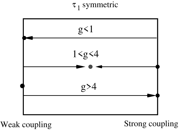
Figure 3: RG flow for $B_{\parallel}=0=B_{\perp}=0$. The boundary interaction flows towards weak coupling for $g<1$, towards strong coupling for $g>4$, while, for $1<g<4$, the RG flow points towards a finite coupling fixed point, represented as a gray circle.

Figure 4: RG flow diagram for various values of the Luttinger parameter $g$ and of the control parameters $B_{\parallel},B_{\perp}$: Left panel: RG flow diagram for $B_{\parallel}\neq 0,B_{\perp}\neq 0$; Middle panel: Flow diagram for $B_{\parallel}=0,B_{\perp}\neq 0$; Right panel: Flow diagram for $B_{\parallel}\neq 0,B_{\perp}=0$.

In summary, our analysis evidences that a FFP emerges only when the SIs are a relevant boundary perturbation to the SFP. As shown in appendix B, this happens only over length scales $L$ such that $L_{*}\leq L\leq L_{\rm Stop}\sim L_{0}\left(\frac{1}{g_{1}\cos(\theta)}\right)$. For $B_{\parallel}\to 0$, $L_{\rm Stop}\to\infty$, and, thus, the FFP becomes a stable, attractive fixed point.

3.3 Frustration of decoherence near by the finite coupling fixed point

In this subsection, we focus on the analysis of the interaction between the spin-1/2 degree of freedom sitting at $x=0$ (${\bf S}$), and the plasmon modes of the leads, which may be regarded as a bath of this two-level quantum mechanical system. We shall show that, near by the FFP (i.e., for $1<g<4$ and for $B_{\parallel}=0$), the decoherence induced by the plasmon bath is drastically reduced [33, 34]. To do this, we compute the spectral density of states (SDOS) of the local spin-1/2 variable, which is given by

$$S(\Omega)=\Im m\left[\frac{[\chi^{\rm Tr}](i\Omega+0^{+})}{\Omega}\right]\>\>\>\>,$$ (24)

where $[\chi^{\rm Tr}](\Omega)$ is the transverse spin susceptibility, defined as

$$[\chi^{\rm Tr}](\Omega)=\int_{0}^{\infty}\>d\tau\>e^{i\Omega\tau}\>\langle{\bf T}_{\tau}[\{\cos(\theta){\bf S}_{G}^{x}(\tau)-\sin(\theta){\bf S}_{G}^{z}(\tau)\}\{\cos(\theta){\bf S}_{G}^{x}(0)-\sin(\theta){\bf S}_{G}^{z}(0)\}]\rangle\>\>\>\>.$$ (25)

To carry out our task, it is most convenient to compute $[\chi^{\rm Tr}](\Omega)$ for $g=1,4$, and then to extrapolate the behavior of $S(\Omega)$ for any $1<g<4$.

For $g=1$, $\cos[2\Phi(0)]$ is an irrelevant perturbation and one may safely assume that the FFP should lie at a distance $O(g_{1})$ from the WFP, so that Neumann BCs may be imposed on $\Phi$ at $x=0$. As a result, one gets the simplified boundary action given by

$$S_{\bf B}=S^{(0)}_{\bf B}-\frac{g_{1}}{2}\int_{0}^{\beta}\>d\tau\>\{a^{\dagger}a-b^{\dagger}b\}[:e^{i\Phi(\tau)}:+:e^{-i\Phi(\tau)}:]\>\>\>\>,$$ (26)

with the operators $:e^{\pm i\Phi(0)}:$ having scaling dimension equal to 1. Similarly, for $g=4$, $:e^{\frac{i}{2}\Theta(0)}:$ has scaling dimension 1, and the Euclidean boundary action is given by the dual of Eq.(26), namely

$$\tilde{S}_{\bf B}=S^{(0)}_{\bf B}-\frac{\mu_{1}}{2}\int_{0}^{\beta}\>d\tau\>\{a^{\dagger}b+b^{\dagger}a\}[:e^{i\Theta(\tau)}:+:e^{-i\Theta(\tau)}:]\>\>\>\>.$$ (27)

By means of a Bogoliubov transformation to the normal modes of the boundary fermions $\alpha,\beta$, one finds

$${\bf S}^{z} = \cos(\theta)\{\alpha^{\dagger}\alpha-\beta^{\dagger}\beta\}-\sin(\theta)\{\alpha^{\dagger}\beta+\beta^{\dagger}\alpha\}$$

$${\bf S}^{x} = -\sin(\theta)\{\alpha^{\dagger}\alpha-\beta^{\dagger}\beta\}+\cos(\theta)\{\alpha^{\dagger}\beta+\beta^{\dagger}\alpha\}\>\>\>\>,$$ (28)

with

$$\alpha=\cos(\frac{\theta}{2})a+\sin(\frac{\theta}{2})b\;\;\;,\;\;\beta=-\sin(\frac{\theta}{2})a+\cos(\frac{\theta}{2})b\>\>\>\>,$$ (29)

For $g=1$, one may resort to the random phase approximation (RPA) used in Ref.[33] to compute the “dressed” transverse spin susceptibility (plotted in Fig.5):

$$\chi^{\rm Tr}(\Omega)=\frac{[\chi^{\rm Tr}]^{(0)}(\Omega)}{1+\frac{g_{1}^{2}\sin^{2}(\theta)}{4}|\Omega|[\chi^{\rm Tr}]^{(0)}(\Omega)}\>\>\>\>,$$ (30)

where $[\chi^{\rm Tr}]^{(0)}(\Omega)$ is given by

$$[\chi^{\rm Tr}]^{(0)}(\Omega)=\int_{0}^{\infty}\>d\tau\>e^{i\Omega\tau}\>\langle{\bf T}_{\tau}[\{\cos(\theta){\bf S}^{x}(\tau)-\sin(\theta){\bf S}^{z}(\tau)\}\{\cos(\theta){\bf S}^{x}(0)-\sin(\theta){\bf S}^{z}(0)\}]\rangle_{(0)}$$

$$=\frac{4\lambda}{\Omega^{2}+4\lambda^{2}}\>\>\>\>.$$ (31)

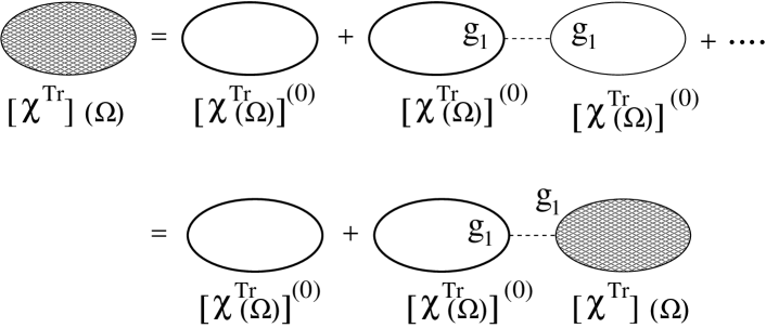
Figure 5: Diagrams in the RPA sum yielding Eq.(30).

From Eqs.(24,31), one gets

$$S(\Omega)=\frac{\Im m[\chi^{\rm Tr}(-i\Omega+0^{+})]}{\Omega}=\frac{4\lambda\frac{\sin^{2}(\theta)g_{1}^{2}}{4}}{(-\Omega^{2}+4\lambda^{2})^{2}+\left(\frac{g_{1}^{2}\sin^{2}(\theta)}{4}\right)\Omega^{2}}\>\>\>\>.$$ (32)

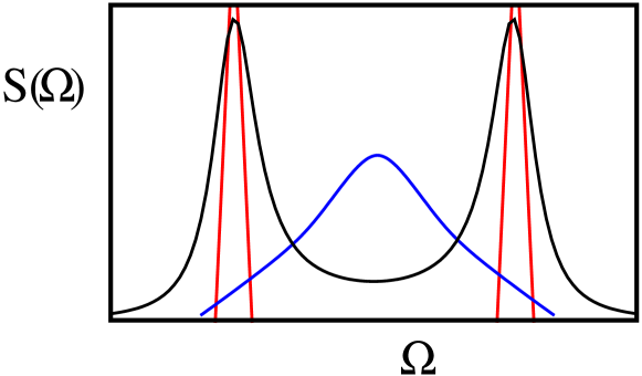
Figure 6: Plot of the spectral density $S(\Omega)$ in the various regime accessible to the device: Blue line: $S(\Omega)$ near by the WFP; Red line: $S(\Omega)$ near by the SFP; Black line: $S(\Omega)$ near by the FFP (see Ref.[34] for details).

A plot of $S(\Omega)$ vs. $\Omega$ is reported in Fig.6. One sees that the limited broadening of the two peaks at $\Omega\sim 2\lambda$ (which is the signal of frustration of decoherence) depends on having both $g_{1}$ finite, and $\sin(\theta)\neq 0$. Furthermore, choosing $g=1$, implies that $g_{1}$ is the coefficient of a marginal perturbation and, thus, is not renormalized by the interaction.

For $g>1$, the system is attracted by an IR stable FFP and one has that $g_{1}$ goes to $g_{1}^{*}$, where $g_{1}^{*}$ is the value of this coupling at the FFP. Even if in section 3 it has been shown that the FFP is IR attractive only when $B_{\parallel}=B_{\perp}=0$, the evaluation of the”dressed”transverse spin susceptibility requires to slightly move from the FFP by applying a small, nonzero $B_{\parallel}$ and/or $B_{\perp}$, in order to split the two impurity levels [33]. This may be safely carried out when the JJN has a finite size L since, in this case, the FFP is stable also against small fluctuations of the control parameters $B_{\parallel},B_{\perp}$, provided that $u/L$ is sufficiently big (see appendix B). As a result, for $g>1$, the equation yielding $S(\Omega)$ has the same form as Eq.(32), provided one replaces $g_{1}$ with $g_{1}^{*}$ and introduces a “self-energy correction” $\propto|\Omega|^{\frac{2}{g}-1}$ [34]. From the duality relations given in Eq.(22), one finds that Eq.(32) holds also for $g=4$. Our results confirm that frustration of decoherence may be a remarkable signature of the emergence of a FFP in the phase diagram accessible to superconducting quantum devices [34].

4 Josephson current and coherent tunneling of Cooper pairs

In section 2, we showed that the Hamiltonian $H_{\bf B}$ is invariant under the $\tau_{1}$-symmetry, even if it contains a term $\propto\cos[\Phi(0)]$. In the following, we show that this symmetry is responsible for the appearance of $4e$ superconducting correlations in all the phases accessible to the JJN. For this purpose, we shall compute the Josephson current (JC) across C in all the phases of the JJN.

To induce a JC, one may connect the leads of the JJN to two bulk superconductors at fixed phase difference $\alpha$ (see Fig.1) [10, 13]. This amounts to require that, at the outer boundary ($x=L$), $\Phi(L,t)=\alpha$. The (0-temperature) dc JC $I(\alpha)$ may then be computed as

$$I(\alpha)=-\lim_{\beta\to\infty}\frac{e^{*}}{\beta}\frac{\partial\ln{\bf Z}}{\partial\alpha}\>\>\>\>,$$ (33)

with $e^{*}=2e$ being the Cooper pair charge and ${\bf Z}$ defined in Eq.(5)

4.1 DC Josephson current near by the weakly coupled fixed point

Near by the WFP, $\Phi(x,\tau)$ is given by

$$\Phi(x,\tau)=\alpha+\sum_{n\in{\bf Z}}\frac{\alpha(n)}{n+\frac{1}{2}}\cos\left[\left(n+\frac{1}{2}\right)\frac{\pi x}{L}\right]e^{-\left(n+\frac{1}{2}\right)\frac{\pi u\tau}{L}}\>\>\>\>,$$ (34)

with

$$[\alpha(n),\alpha(n^{\prime})]=\delta_{n+n^{\prime}-1}\left(n+\frac{1}{2}\right)\>\>\>\>.$$

Taking into account that $\langle:e^{ia\Phi(0,\tau)}:\rangle_{(0)}=e^{ia\alpha}$, one gets

$$\ln{\bf Z}\approx\ln{\bf Z}_{0}+y_{1}\int_{0}^{\beta}\;d\tau\>\langle:\cos\left[\Phi(0,\tau)\right]:\rangle_{(0)}+y_{2}\int_{0}^{\beta}\;d\tau\>\langle:\cos\left[2\Phi(0,\tau)\right]:\rangle_{(0)}$$

$$=\ln{\bf Z}_{0}+\beta\{y_{1}\cos(\alpha)+y_{2}\cos(2\alpha)\}\>\>\>\>,$$ (35)

from which the dc JC is given by

$$I(\alpha)\approx e^{*}y_{1}\sin(\alpha)+2e^{*}y_{2}\sin(2\alpha)\;\;\;\;.$$ (36)

By inspection of Eq.(36), one sees that $I(\alpha)$ is the sum of a term ($\propto\sin(\alpha)$) corresponding to the usual tunneling of Cooper pairs (of charge $e^{*}$) across C, and of a term ($\propto\sin(2\alpha)$) describing the coherent tunneling of pairs of Cooper pairs (CTCP) (of total charge $2e^{*}$) across C. The relative weight of the two terms contributing to $I(\alpha)$ is $\propto\frac{y_{1}}{y_{2}}\propto\cos(\theta)$. Thus, it may be tuned upon acting on $\varphi$ till, at $\varphi=\pi$, only the term $\propto\sin(2\alpha)$ is left, that is, the JC flows across C only because of CTCP. In Fig.7, we plot the dc JC across C for different values of $\varphi$.

Figure 7: Plot of the dc Josephson current across C at the WFP for $\bar{g}_{2}/\bar{g}_{1}=.3$ and for different values of $B_{\parallel}/B_{\perp}$. a): Top left panel: $B_{\parallel}/B_{\perp}=10$; b): Bottom left panel: $B_{\parallel}/B_{\perp}=.1$; c): Bottom right panel: $B_{\parallel}/B_{\perp}=.05$; d): Top right panel: $B_{\parallel}/B_{\perp}=0$.

The CTCP is also evidenced in the ac JC, arising across C when a finite voltage bias $V$ is applied to the ends of both leads. To account for $V$, one has simply to add to $H_{\rm BDSG}$ a “voltage bias” term $H_{V}=\frac{ge^{*}V}{2\pi}\frac{\partial\Phi}{\partial t}$, which yields a time-dependent shift of $\Phi$ as $\Phi\to\Phi+e^{*}Vt$, from which the ac JC is given by

$$I(\alpha,t)\to I(\alpha+e^{*}Vt)=e^{*}y_{1}\sin(\alpha+e^{*}Vt)+2e^{*}y_{2}\sin(2\alpha+2e^{*}Vt)\;\;\;\;.$$ (37)

4.2 DC Josephson current near by the strongly coupled fixed point

Near by the SFP, the field $\Phi$, given by Eq.(38), contains contributions from the zero mode operator. As a result, the partition function may be factorized as ${\bf Z}={\bf Z}_{\rm 0-mode}[\alpha]{\bf Z}_{\rm osc}$, where ${\bf Z}_{\rm 0-mode}[\alpha]$ is the contribution of the zero-mode operators. From the analysis of the zero mode spectrum carried in subsection 3.2, one sees that, for $B_{\parallel}\geq 0$, the eigenvalues of the zero-mode operator $P$ are given by $\{p_{k}\}=\{\sqrt{g}(k+\alpha/\pi)\}$, with the odd-$k$ eigenvalues higher in energy by $\Delta\epsilon=\bar{g}_{1}\cos(\theta)$. As a result

Figure 8: Plot of the dc Josephson current across C at the SFP for (from top left panel to top right panel, rotating counterclockwisely) $\Delta\epsilon/\frac{\pi u}{4L}\gg 1$; $\Delta\epsilon/\frac{\pi u}{4L}\sim 1$; $\Delta\epsilon/\frac{\pi u}{4L}\ll 1$; $\Delta\epsilon/\frac{\pi u}{4L}=0$.

$${\bf Z}_{\rm 0-mode}[\alpha]=\sum_{k\in Z}\>\exp\left[-\beta\left(\frac{\pi u}{4L}(p_{k})^{2}+[1-(-1)^{k}]\frac{\Delta\epsilon}{2}\right)\right]\>\>\>\>,$$ (38)

from which the dc JC is obtained as

$$I(\alpha)=\lim_{\beta\to\infty}\frac{e^{*}}{\beta}\frac{\partial\ln{\bf Z}_{\rm 0-mode}[\alpha]}{\partial\alpha}\>\>\>\>.$$ (39)

In Fig.8 we plot $I(\alpha)$ vs. $\alpha$ for different values of $\Delta\epsilon/\frac{\pi u}{4L}$. One notices that for $\Delta\epsilon/\frac{\pi u}{4L}\gg 1$, the current takes the usual sawtooth behavior with periodicity in $\alpha$ equal to $2\pi$. Furthermore, as $\Delta\epsilon/\frac{\pi u}{4L}\sim 1$, one sees that the current continuously crosses $\alpha=\pi$, with “satellite” jumps at $\alpha=\pi\pm\left[\frac{\pi}{2}-\frac{4L\Delta\epsilon}{\pi ug}\right]$. As $\Delta\epsilon/\frac{\pi u}{4L}$ approaches 0, the satellite jumps move to $\pi\pm\pi/2$, where they eventually take place, when $\Delta\epsilon=0$. As a result, the period of the sawtooth is exactly halved at $\Delta\epsilon/\frac{\pi u}{4L}=0$.

4.3 DC Josephson current near by the finite coupling fixed point

To compute the JC near by the FFP, one must include the effects of the relevant SI perturbation at the SFP. While long instantons just provide a smoothing of the spikes of $I(\alpha)$ at the SFP [34], for $B_{\parallel}=0$ and $B_{\perp}=0$, SIs become a relevant perturbation and drive the system to the IR attractive FFP. As a result, for $B_{\parallel}=0$ and $B_{\perp}=0$, one expects that the net effect of the SIs on the dc JC will be to smoothen the sharp jumps of the sawtooth depicted in Fig.8, while still preserving the half periodicity of $I(\alpha)$.

In the following, we compute $I(\alpha)$ near by the jump at $\alpha=\pi/2$ for $\Delta\epsilon/\frac{\pi u}{4L}=0$ (top right panel of Fig.8). Upon tuning $\alpha$ so that $0<\alpha<\pi$, the low energy states contributing to $I(\alpha)$ are associated with the zero modes labeled by $p_{k}=p_{0}$ and $p_{k}=-1$. Their energies are respectively given by $E_{0}(\alpha)\pm\epsilon_{0}(\alpha)$, with

$$E_{0}(\alpha)=\frac{g}{4\pi L}\left[\frac{\pi^{2}}{4}+\left(\frac{\pi}{2}-\alpha\right)^{2}\right]\;\;\;,\;\;\epsilon_{0}(\alpha)=\frac{g}{4\pi L}\left(\frac{\pi}{2}-\alpha\right)\>\>\>\>.$$ (40)

Since, for $p=p_{0}$, ${\bf S}^{z}=1$, while, $p=p_{-1}$, ${\bf S}^{z}=-1$, one may trade the degeneracy-breaking energy $\epsilon_{0}(\alpha)$ with an effective $B_{\parallel}(\alpha)=\epsilon_{0}(\alpha)$; in addition, as one is approaching the FFP from the SFP, one should take, as boundary interaction, the dual boundary Hamiltonian $\tilde{H}_{\bf B}$ given in Eq.(21); the term ($\propto\cos[\Theta(0)/2]$) now acts on the spin ${\bf S}$ as an effective field $B_{\perp}\sim\bar{\mu}_{1}$. As a result, one may compute $I(\alpha)$ for $\alpha\sim\pi/2$ by taking the logarithmic derivative with respect to $\alpha$ of the relevant contribution to ${\bf Z}_{\rm 0-mode}[\alpha]$; namely

$${\bf Z}_{\rm 0-mode}[\alpha]\sim e^{-\beta E_{0}(\alpha)}\int\>{\bf D}\{a,b\}\>e^{-S_{E}[\{a,b\}]+\ldots}\>\>\>\>,$$ (41)

with

$$S_{E}[\{a,b\}]=\int_{0}^{\beta}\>d\tau\>\left\{a^{\dagger}\left[\frac{\partial}{\partial\tau}-B_{\parallel}(\alpha)\right]a+b^{\dagger}\left[\frac{\partial}{\partial\tau}+B_{\parallel}(\alpha)\right]b+B_{\perp}[a^{\dagger}b+b^{\dagger}a]\right\}\>\>\>\>,$$ (42)

while the ellipses denote contributions coming from $p_{k}\neq\{p_{0},p_{-1}\}$. Using Eq.(33), one gets

$$I(\alpha)\approx-\frac{e^{*}g}{2\pi L}\left(\alpha-\frac{\pi}{2}\right)\left\{1+\frac{\left(\alpha-\frac{\pi}{2}\right)}{\left(\alpha-\frac{\pi}{2}\right)^{2}+\left(\frac{4\pi\mu_{1}}{g}\right)^{2}L^{2-\frac{g}{2}}}\right\}\>\>\>\>.$$ (43)

Eq.(43) shows that $I(\alpha)$ is a smooth function, linearly crossing 0, at $\alpha=\pi/2$. The term $\propto L^{2-\frac{g}{2}}$ in the denominator evidences that this behavior is more pronounced, as the system size increases. Carrying out a similar computation for $\alpha\neq\pi/2$ leads to the plot displayed in Fig.9.

Figure 9: Sketch of $I(\alpha)$ vs. $\alpha$ near by the FFP (Eq.(43)).

In the next section, we shall show how the results obtained for the coherent current transport in the JJN extend to the situation in which a dissipative current is induced, as well.

5 DC transport and coherent tunneling of Cooper pairs

In this section, we analyze the observable consequences of CTCP on a dc transport experiment. For this purpose, we shall compute the dissipative current $I_{\rm DC}(V)$ flowing across C when the leads are connected to two metallic wires, at fixed voltage bias $V$. Differently from the Josephson supercurrent, $I_{\rm DC}(V)$ fluctuates even at $T=0$, in presence of weak tunneling and/or backscattering centers, and this zero-temperature fluctuations are measured by the shot noise at voltage bias $V$ and frequency $\Omega$,

$$S(V,\Omega)=\int\>dt\>e^{i\Omega t}\langle\{I_{\rm fl}(t),I_{\rm fl}(0)\}\rangle_{\rm NE}\>\>\>\>,$$ (44)

where $\{,\}$ is the anticommutator, $\langle\ldots\rangle_{\rm NE}$ denotes averaging, at zero temperature and at finite $V$, $I_{\rm fl}$ is either identified with the transmitted current, when the two leads are weakly coupled to each other, or with the backscattered current, when the leads are strongly coupled.

Measuring the shot noise provides a tool to probe the effective elementary charge $q$ flowing across a device since, from the functional dependence of $S(V,\Omega)$ upon $V$, one obtains $q$ as

$$q(V)=S(V,\Omega\to 0)/(2I_{\rm fl}(V))\>\>\>\>.$$ (45)

Measurements of $S$ have been used to probe noninteger charges in fractional quantum Hall bars [28], in normal metal-superconductor junctions [29], in Kondo dots [27]. In the following, we show that, by properly tuning the external control parameter, pairing of Cooper pairs may be as well detected in a shot noise measurement, provided that $V$ is lower than a threshold, depending on the values of $B_{\parallel}$ and $B_{\perp}$.

In subsection 5.1, we compute $I_{\rm fl}(V)$ and $S(V)$ at finite $V$ near by the WFP. We show that, when $B_{\parallel}=0$, $B_{\perp}$ defines a threshold below which the effective charge detected from a shot noise measurement is $q=2e^{*}$, which evidences a phase with $4e$ superconductivity.

In subsection 5.2, we use the fermionization procedure of the BDSG Hamiltonian for $g=2$ [36], to extend the results of subsection 5.1 beyond the perturbative regime in the boundary couplings. Mathematical details concerning the derivation of subsection 5.1 are provided in appendix C, while the fermionization procedure is discussed in detail in appendix D.

5.1 Perturbative computation of the dissipative current and of the shot noise at finite voltage bias $V$

When the JJN is connected to two metallic wires at finite voltage bias $V$, the computation of the current flowing across C -and its fluctuations- may be carried out within the Hamiltonian formalism. In particular, near by the WFP, one may consistently compute both $I_{\rm DC}(V)$ and $S(V)$ nonperturbatively in $V$, resorting to time-dependent perturbation theory in the boundary couplings $g_{1}$, $g_{2}$.

Applying a finite voltage bias $V$ amounts to shift the field $\Phi$ as $\Phi\to\Phi+\omega_{V}t$, with $\omega_{V}=e^{*}V$. To the leading order in $g_{1},g_{2}$, the current operator in the Heisenberg representation, $j_{H}(t)$, is obtained by

$$j_{H}(t)\approx j_{I}(t)+i\int_{-\infty}^{t}\>d\tau\>[H_{\bf B}(\tau),j_{I}(t)]\>\>\>\>,$$ (46)

where $j_{I}(t)$ and $H_{\bf B}(t)$ are, respectively, the current operator and the boundary Hamiltonian in the interaction representation, given by

$$j_{I}(t) = e^{*}\bar{g}_{1}{\bf S}^{z}(t):\sin[\Phi(t)+\omega_{V}t]:+2e^{*}\bar{g}_{2}:\sin[2\Phi(t)+2\omega_{V}t]:$$

$$H_{\bf B}(t) = -\bar{g}_{1}{\bf S}^{z}(t):\cos[\Phi(t)+\omega_{V}t]:-\bar{g}_{2}:\cos[2\Phi(t)+2\omega_{V}t]:\>\>\>\>,$$ (47)

with $\Phi(t)\equiv\Phi(x=0,t)$.

The 0-temperature average value of $j_{H}(t)$ is given by

$$I_{\rm DC}(V)=-e^{*}\cos^{2}(\theta)\bar{g}_{1}^{2}\>\Re e\left\{\int_{0}^{\infty}\>d\tau\>\frac{[e^{i\omega_{V}\tau}-e^{-i\omega_{V}\tau}]}{[e^{\frac{\pi iu}{L}\tau}-e^{-\frac{\pi iu}{L}(\tau-i\eta)}]^{\frac{2}{g}}}\right\}$$

$$-e^{*}\sin^{2}(\theta)\bar{g}_{1}^{2}\>\Re e\left\{\int_{0}^{\infty}\>d\tau\>\frac{e^{-2i\lambda\tau}[e^{i\omega_{V}\tau}-e^{-i\omega_{V}\tau}]}{[e^{\frac{\pi iu}{L}\tau}-e^{-\frac{\pi iu}{L}(\tau-i\eta)}]^{\frac{2}{g}}}\right\}$$

$$-2e^{*}\bar{g}_{2}^{2}\>\Re e\left\{\int_{0}^{\infty}\>d\tau\>\frac{[e^{2i\omega_{V}\tau}-e^{-2i\omega_{V}\tau}]}{[e^{\frac{\pi iu}{L}\tau}-e^{-\frac{\pi iu}{L}(\tau-i\eta)}]^{\frac{8}{g}}}\right\}\>\>\>\>,$$ (48)

while $S(V)$ is given by

$$S(V)=-2(e^{*})^{2}\cos^{2}(\theta)\bar{g}_{1}^{2}\>\Re e\left\{\int_{0}^{\infty}\>d\tau\>\frac{[e^{i\omega_{V}\tau}+e^{-i\omega_{V}\tau}]}{[e^{\frac{\pi iu}{L}\tau}-e^{-\frac{\pi iu}{L}(\tau-i\eta)}]^{\frac{2}{g}}}\right\}$$

$$-2(e^{*})^{2}\sin^{2}(\theta)\bar{g}_{1}^{2}\>\Re e\left\{\int_{0}^{\infty}\>d\tau\>\frac{e^{-2i\lambda\tau}[e^{i\omega_{V}\tau}+e^{-i\omega_{V}\tau}]}{[e^{\frac{\pi iu}{L}\tau}-e^{-\frac{\pi iu}{L}(\tau-i\eta)}]^{\frac{2}{g}}}\right\}$$

$$-8(e^{*})^{2}\bar{g}_{2}^{2}\>\Re e\left\{\int_{0}^{\infty}\>d\tau\>\frac{[e^{2i\omega_{V}\tau}+e^{-2i\omega_{V}\tau}]}{[e^{\frac{\pi iu}{L}\tau}-e^{-\frac{\pi iu}{L}(\tau-i\eta)}]^{\frac{8}{g}}}\right\}\>\>\>\>.$$ (49)

The relevant integrals needed in Eqs.(48,49) are computed in appendix C. As a result, $I_{\rm DC}(V)$ and $S(V)$ are given by

$$I_{\rm DC}(V)=e^{*}\cos^{2}(\theta)\bar{g}_{1}^{2}\>\Re e\biggl{\{}i\biggl{[}\frac{\Gamma[1-\frac{2}{g}]\>\Gamma[\frac{L\omega_{V}}{2\pi u}+\frac{1}{g}+1]}{\left(\omega_{V}-\frac{2\pi u}{gL}\right)\Gamma[\frac{L\omega_{V}}{2\pi u}-\frac{1}{g}+1]}+\frac{\Gamma[1-\frac{2}{g}]\>\Gamma[-\frac{L\omega_{V}}{2\pi u}+\frac{1}{g}+1]}{\left(\omega_{V}+\frac{2\pi u}{gL}\right)\Gamma[-\frac{L\omega_{V}}{2\pi u}-\frac{1}{g}+1]}\biggr{]}\biggr{\}}$$

$$+e^{*}\bar{g}_{1}^{2}\sin^{2}(\theta)\>\Re e\biggl{\{}i\biggl{[}\frac{\Gamma[1-\frac{2}{g}]\>\Gamma[\frac{L(\omega_{V}+2\lambda)}{2\pi u}+\frac{1}{g}+1]}{\left(\omega_{V}+2\lambda-\frac{2\pi u}{gL}\right)\Gamma[\frac{L(\omega_{V}+2\lambda)}{2\pi u}-\frac{1}{g}+1]}$$

$$+\frac{\Gamma[1-\frac{2}{g}]\>\Gamma[-\frac{L(\omega_{V}-2\lambda)}{2\pi u}+\frac{1}{g}+1]}{\left(\omega_{V}-2\lambda+\frac{2\pi u}{gL}\right)\Gamma[-\frac{L(\omega_{V}-2\lambda)}{2\pi u}-\frac{1}{g}+1]}\biggr{]}\biggr{\}}$$

$$+2e^{*}\bar{g}_{2}^{2}\>\Re e\biggl{\{}i\biggl{[}\frac{\Gamma[1-\frac{8}{g}]\>\Gamma[\frac{L\omega_{V}}{\pi u}+\frac{4}{g}+1]}{\left(2\omega_{V}-\frac{8\pi u}{gL}\right)\Gamma[\frac{L\omega_{V}}{\pi u}-\frac{4}{g}+1]}+\frac{\Gamma[1-\frac{8}{g}]\>\Gamma[-\frac{L\omega_{V}}{\pi u}+\frac{4}{g}+1]}{\left(2\omega_{V}+\frac{8\pi u}{gL}\right)\Gamma[-\frac{L\omega_{V}}{\pi u}-\frac{4}{g}+1]}\biggr{]}\biggr{\}}\>\>\>\>,$$ (50)

and

$$S(V)=2(e^{*})^{2}\cos^{2}(\theta)\bar{g}_{1}^{2}\>\Re e\biggl{\{}i\biggl{[}-\frac{\Gamma[1-\frac{2}{g}]\>\Gamma[\frac{L\omega_{V}}{2\pi u}+\frac{1}{g}+1]}{\left(\omega_{V}-\frac{2\pi u}{gL}\right)\Gamma[\frac{L\omega_{V}}{2\pi u}-\frac{1}{g}+1]}-\frac{\Gamma[1-\frac{2}{g}]\>\Gamma[-\frac{L\omega_{V}}{2\pi u}+\frac{1}{g}+1]}{\left(\omega_{V}+\frac{2\pi u}{gL}\right)\Gamma[-\frac{L\omega_{V}}{2\pi u}-\frac{1}{g}+1]}\biggr{]}\biggr{\}}$$

$$+2(e^{*})^{2}\bar{g}_{1}^{2}\sin^{2}(\theta)\>\Re e\biggl{\{}i\biggl{[}-\frac{\Gamma[1-\frac{2}{g}]\>\Gamma[\frac{L(\omega_{V}+2\lambda)}{2\pi u}+\frac{1}{g}+1]}{\left(\omega_{V}+2\lambda-\frac{2\pi u}{gL}\right)\Gamma[\frac{L(\omega_{V}+2\lambda)}{2\pi u}-\frac{1}{g}+1]}$$

$$+\frac{\Gamma[1-\frac{2}{g}]\>\Gamma[-\frac{L(\omega_{V}-2\lambda)}{2\pi u}+\frac{1}{g}+1]}{\left(\omega_{V}-2\lambda+\frac{2\pi u}{gL}\right)\Gamma[-\frac{L(\omega_{V}-2\lambda)}{2\pi u}-\frac{1}{g}+1]}\biggr{]}\biggr{\}}$$

$$+8(e^{*})^{2}\bar{g}_{2}^{2}\>\Re e\biggl{\{}i\biggl{[}-\frac{\Gamma[1-\frac{8}{g}]\>\Gamma[\frac{L\omega_{V}}{\pi u}+\frac{4}{g}+1]}{\left(2\omega_{V}-\frac{8\pi u}{gL}\right)\Gamma[\frac{L\omega_{V}}{\pi u}-\frac{4}{g}+1]}+\frac{\Gamma[1-\frac{8}{g}]\>\Gamma[-\frac{L\omega_{V}}{\pi u}+\frac{4}{g}+1]}{\left(2\omega_{V}+\frac{8\pi u}{gL}\right)\Gamma[-\frac{L\omega_{V}}{\pi u}-\frac{4}{g}+1]}\biggr{]}\biggr{\}}\>\>\>\>.$$ (51)

Finally, the Stirling’s approximation (Eq.(101)) allows to derive the large-$L$ limit ($(L\omega_{V}/2\pi u)\gg 1$) of Eqs.(50,51), leading to

$$I_{\rm DC}(V)\approx e^{*}\Gamma[1-\frac{2}{g}]\sin\left(\frac{2\pi}{g}\right)\biggl{\{}\frac{\bar{g}_{1}^{2}\cos^{2}(\theta)}{\omega_{V}}\left(\frac{L\omega_{V}}{2\pi u}\right)^{\frac{2}{g}}$$

$$+\frac{\bar{g}_{1}^{2}\sin^{2}(\theta)}{\omega_{V}-2\lambda}\>\theta(\omega_{V}-2\lambda)\left(\frac{L(\omega_{V}-2\lambda)}{2\pi u}\right)^{\frac{2}{g}}\biggr{\}}+2e^{*}\Gamma[1-\frac{8}{g}]\sin\left(\frac{8\pi}{g}\right)\frac{\bar{g}_{2}^{2}}{2\omega_{V}}\left(\frac{L\omega_{V}}{\pi u}\right)^{\frac{8}{g}}\>\>\>\>,$$ (52)

and

$$S(V)\approx 2(e^{*})^{2}\Gamma[1-\frac{2}{g}]\sin\left(\frac{2\pi}{g}\right)\biggl{\{}\frac{\bar{g}_{1}^{2}\cos^{2}(\theta)}{\omega_{V}}\left(\frac{L\omega_{V}}{2\pi u}\right)^{\frac{2}{g}}$$

$$+\frac{\bar{g}_{1}^{2}\sin^{2}(\theta)}{\omega_{V}-2\lambda}\>\theta(\omega_{V}-2\lambda)\left(\frac{L(\omega_{V}-2\lambda)}{2\pi u}\right)^{\frac{2}{g}}\biggr{\}}+8(e^{*})^{2}\Gamma[1-\frac{8}{g}]\sin\left(\frac{8\pi}{g}\right)\frac{\bar{g}_{2}^{2}}{2\omega_{V}}\left(\frac{L\omega_{V}}{\pi u}\right)^{\frac{8}{g}}\>\>\>\>,$$ (53)

with $\theta(x)$ being Heavside’s $\theta$-function.

To determine $q(V)$, one observes that the term $\propto\bar{g}_{1}^{2}\sin^{2}(\theta)$ in Eqs.(52,53) exhibits a threshold at $\omega_{V}=2\lambda$. In computing $q(V)$, one notices that, since the term $\propto\cos[\Phi(0)]$ and the term $\propto\cos[2\Phi(0)]$ in $H_{\bf B}$ have different scaling dimensions ($1/g$ and $4/g$, respectively), tuning the low-energy scale $\omega_{V}$ induces a flow in $q(V)$. Indeed, assuming $B_{\parallel}\neq 0$, one finds that $q(V)\sim e^{*}$ for $\omega_{V}\ll\omega_{*}$, while $q(V)\sim 2e^{*}$ for $\omega_{V}\gg\omega*$, with the crossover scale $\omega_{*}$ given by

$$\omega_{*}\sim\frac{\pi u}{L}\left[\frac{\bar{g}_{1}^{2}\cos^{2}(\theta)}{\bar{g}_{2}^{2}}\frac{\Gamma[1-\frac{8}{g}]}{\Gamma[1-\frac{2}{g}]}\frac{\sin\left(\frac{8\pi}{g}\right)}{\sin\left(\frac{2\pi}{g}\right)}\right]^{\frac{6}{g}}\>\>\>\>.$$ (54)

Eq.(54) states that the contributions to $I_{\rm DC}(V)$ and to $S(V)$, which are $\propto\bar{g}_{1}^{2}\cos^{2}(\theta)$ and $\propto\bar{g}_{2}^{2}$ respectively, are of the same order of magnitude.

As $\omega_{V}\to 0$, the value of $q(V)$ characterizing the IR stable fixed point is always $q=e^{*}$, except when $B_{\parallel}=0,B_{\perp}\neq 0$, where, the existence of a threshold at $\omega_{V}=2\lambda$ implies that $q(V)=2e^{*}$, for $\omega_{V}\leq 2\lambda=2|B_{\perp}|$. Thus, for $B_{\parallel}=0,B_{\perp}\neq 0$ $4e$ superconductivity is evidenced in the dissipative dc transport as well, when $\omega_{V}\leq 2\lambda$. $q(V)$ is plotted in Fig.10, both for $B_{\parallel}\neq 0$, and for $B_{\parallel}=0,B_{\perp}\neq 0$. For $B_{\parallel}=0,B_{\perp}=0$, the threshold at $\omega_{V}=2\lambda$ moves to $\omega_{V}=0$. This is again consistent with the picture of a $4e$-deconfined superconductor, with $2e$ elementary charged excitations (see section 3.2).

Figure 10: Plot of $q(V)\equiv S(V)/I_{\rm DC}(V)$. Left-hand panel: $q(V)$ vs. $\omega_{V}$ for $B_{\parallel}\neq 0$ ($\tau_{1}$-symmetry explicitly broken); Right-hand panel: $q(V)$ vs. $\omega_{V}$ for $B_{\parallel}=0$ ($\tau_{1}$-symmetric case). While for $B_{\parallel}\neq 0$ $q(V)$ flows from $e^{*}$ (low-voltage limit) to $2e^{*}$, for $B_{\parallel}=0$ and $B_{\perp}\neq 0$ $q(V)=2e^{*}$ also for $|\omega_{V}|\leq 2\lambda=2|B_{\perp}|$.

5.2 Exact formula for $I_{\rm DC}(V)$ and $S(V)$ in the fermionized theory for $g=2$

In this subsection, we use the exact fermionization of the BDSG Hamiltonian at $g=2$ (see appendix D for details), to compute $I_{\rm DC}(V)$ and $S(V)$ beyond perturbation theory, for $B_{\parallel}=0$.

Applying a finite voltage bias $V$ to the leads amounts to add to the fermionic action $S^{\rm Fer}$ given in Eq.(109), a contribution given by

$$S_{V}=\frac{e^{*}V}{2}\>\int\>dt\>\int_{0}^{L}\>dx\>[:\psi_{R}^{\dagger}(x,t)\psi_{R}(x,t):+:\psi_{L}^{\dagger}(x,t)\psi_{L}(x,t):]\>\>\>\>.$$ (55)

In the fermionized theory, the current operator $j_{H}(t)$ is given by

$$j_{H}(t)=e^{*}u\{:\psi_{R}^{\dagger}(0,t)\psi_{R}(0,t):-:\psi_{L}^{\dagger}(0,t)\psi_{L}(0,t):\}\>\>\>\>.$$ (56)

Taking into account that the finite voltage bias shifts the chemical potential of the $~{}_{R}$ ($~{}_{L}$) modes by $e^{*}V/2$ ($-e^{*}V/2$) and using the linear relations between the right-handed modes $\psi_{R}(p)$ and the left-handed modes $\psi_{L}(p)$ provided in Eq.(112), one obtains that the average current $I_{\rm DC}(V)$ is given by

$$I_{\rm DC}(V)=\frac{e^{*}u}{L}\>\sum_{0\leq p\leq(e^{*}V/2u)}\>[1-|R(p)|^{2}+|Q(p)|^{2}]=\frac{2e^{*}u}{\pi}\int_{0}^{(e^{*}V/2u)}\>dp\>|Q(p)|^{2}\>\>\>\>,$$ (57)

where, to derive Eq.(57), we use $|Q(p)|^{2}=1-|R(p)|^{2}$.

To compute $S(V)$ through Eq.(44), one first needs to determine $S(t,t^{\prime})=\langle\{I_{\rm fl}(t),I_{\rm fl}(t^{\prime})\}\rangle_{\rm NE}$, which, in the fermionized theory, is given by $S(t-t^{\prime})=\Sigma_{1}(t-t^{\prime})+\Sigma_{2}(t-t^{\prime})+\Sigma_{3}(t-t^{\prime})$, with

$$\Sigma_{1}(t-t^{\prime})=-2\left(\frac{e^{*}u}{L}\right)^{2}\sum_{pq}e^{i[\epsilon_{p}-\epsilon_{q}](t-t^{\prime})}[1-R^{*}(p)R(q)+Q^{*}(-p)Q(-q)]\times$$

$$\theta\left(\frac{e^{*}V}{2u}-p\right)\theta\left(-\frac{e^{*}V}{2u}+q\right)\>\>\>\>,$$ (58)

$$\Sigma_{2}(t-t^{\prime})=\Sigma_{3}(t-t^{\prime})$$

$$=2\left(\frac{e^{*}u}{L}\right)^{2}\sum_{pq}e^{i[\epsilon_{p}-\epsilon_{q}](t-t^{\prime})}|R(p)|^{2}|Q(q)|^{2}\theta\left(\frac{e^{*}V}{2u}-p\right)\theta\left(\frac{e^{*}V}{2u}+q\right)\>\>\>\>,$$ (59)

and $\epsilon_{p}=up$.

Taking the Fourier transform of $\Sigma(t-t^{\prime})$ at frequency $\Omega$ and setting $\Omega=0$, one obtains

$$S(V)=S(\Omega\to 0,V)=\frac{4(e^{*})^{2}u}{L}\>\sum_{-(e^{*}V/2u)\leq p\leq(e^{*}V/2u)}\>|Q(p)|^{2}\>|R(p)|^{2}=$$

$$\frac{8(e^{*})^{2}u}{\pi}\>\int_{0}^{(e^{*}V/2u)}\>dp\>\{|Q(p)|^{2}-|Q(p)|^{4}\}\>\>\>\>.$$ (60)

As a result, from Eq.(114) of appendix D, one has

$$I_{\rm DC}(V)=\frac{2e^{*}u}{\pi}\int_{0}^{(e^{*}V/2u)}\>dp\>\ \frac{[-\frac{g_{1}^{2}}{8u}+ug_{2}p^{2}+2B_{\perp}g_{2}p]^{2}}{(up+2B_{\perp})^{2}+[-\frac{g_{1}^{2}}{8u}+ug_{2}p^{2}+2B_{\perp}g_{2}p]^{2}}\>\>\>\>,$$ (61)

and

$$S(V)=\frac{8(e^{*})^{2}u}{\pi}\>\int_{0}^{(e^{*}V/2u)}\>dp\>\frac{(up+2B_{\perp})^{2}[-\frac{g_{1}^{2}}{8u}+ug_{2}p^{2}+2B_{\perp}g_{2}p]^{2}}{\{(up+2B_{\perp})^{2}+[-\frac{g_{1}^{2}}{8u}+ug_{2}p^{2}+2B_{\perp}g_{2}p]^{2}\}^{2}}\>\>\>\>.$$ (62)

Both integrals in Eqs.(61,62) may be exactly computed, although the final expressions are not, in general, very enlightening. However, for $B_{\perp}=0$, one may plot $q(V)$ vs. $V$, obtaining a result matching the left-hand panel of Fig.10; in particular, one finds that

$$\lim_{V\to 0}q(V)=e^{*}\;\;\;,\;\;\lim_{V\to\infty}q(V)=2e^{*}\>\>\>\>.$$ (63)

Eq.(63) shows that the crossover between an effective elementary charge $e^{*}$ and an effective charge $2e^{*}$, induced by acting on the applied voltage bias $V$, is generally valid, independently of the reliability of the perturbative computation of subsection 5.1.

For $B_{\perp}\neq 0$, one obtains

$$\lim_{V\to 0}q(V)=\frac{32e^{*}(2B_{\perp})^{2}}{16\left(\frac{g_{1}^{2}}{8u}\right)^{2}+\frac{g_{1}^{2}}{u}\left(\frac{g_{2}}{u}\right)^{2}(2|B_{\perp}|)+(16+\left(\frac{g_{2}}{u}\right)^{4})(2B_{\perp})^{2}}\>\>\>\>,$$ (64)

which, to the fourth order in $g_{1},g_{2}$, yields

$$\lim_{V\to 0}q(V)=2e^{*}\>\>\>\>.$$ (65)

This is again consistent with the result of Eq.(53), since it shows that $B_{\perp}\neq 0$ may stabilize an IR stable fixed point exhibiting $4e$ superconductivity.

6 Concluding remarks

We investigated a boundary double Sine-Gordon model, where two boundary terms, of different periodicity and scale dimensions, are coupled to a Kondo-like spin degree of freedom. We showed that the pertinent engineering of the coupling between the spin degree of freedom and the bosonic field induces a competition between the two boundary terms, and that this gives rise to nonperturbative phenomena, such as the emergence of novel quantum phases. We showed indeed that the strongly coupled fixed point- in a pertinent range of parameters- becomes unstable as a result of the deconfinement of new phase-slip operators (i.e., the short instantons), arising from adding the less relevant boundary operator.

To look for a physical context where such nonperturbative phenomena may be observed, we analyzed a Josephson junction network, providing a remarkable realization of the BDSG field theory described by $H_{B}$. For this network, we showed that the competition between the two periodicities stabilizes a robust finite coupling fixed point and allows for the emergence, at a pertinent scale, of $4e$ superconductivity. To probe the latter phenomenon, we computed the dc shot noise and showed that, by pertinently tuning the applied voltage bias $V$, the effective charge of the carriers varies from $2e$ to $4e$.

In our analysis the onset of the $\tau_{1}$ symmetry is tuned by acting upon the control parameter $B_{\parallel}$. The role of this symmetry is twofold. In section 3.1 we showed that, for $B_{\perp}\neq 0$, $4e$ superconductivity is naturally associated to the realization of this symmetry. On the other hand, in section 3.2 we showed that, for $B_{\perp}=0$, $\tau_{1}$-symmetry implies SI deconfinement (and, thus, for $1<g<4$ it stabilizes the IR stable FFP); at variance, short instantons are confined, if $\tau_{1}$-symmetry is ”broken”, and the SFP is IR stable for $1<g$.

We argued that while, as the system size $L\to\infty$, the FFP is IR stable only when $B_{\parallel}=B_{\perp}=0$, for a realistic JJN of finite size L, the FFP is robust also against small fluctuations of the control parameters $B_{\parallel},B_{\perp}$, provided that $u/L$ is sufficiently big. Indeed, as discussed in detail in appendix B, SI deconfinement (which is the mechanism de-stabilizing the SFP vs. the FFP) is effective only for $L\geq L_{\rm Stop}\sim 1/(g_{1}^{*}\cos(\theta))$. As a result, for $L\leq L_{\rm Stop}$, one may safely assume that the behavior of the device is still driven by the FFP. This renders the emergence of the FFP in the phase diagram relevant for engineering realistic superconducting devices with enhanced coherence.

It may be worth to investigate how the methods developed in this paper could be modified to account for the effects of different commensurability ratios between competing boundary interactions of a boundary Hamiltonian.

Appendix A Derivation of $H_{\bf B}$

In this appendix, we describe the Schrieffer-Wolff summation procedure, to derive the boundary interaction Hamiltonian $H_{\bf B}$ in Eq.(2). In order to implement this procedure, one should determine the low-energy states of the central region, obtained after diagonalizing the effective spin-1/2 Hamiltonian

$$H_{\bf C}=-J\sum_{j=0}^{3}\{e^{i\frac{\varphi}{4}}S_{j}^{+}S_{j+1}^{\dagger}+{\rm h.c.}\}-h\sum_{j=0}^{3}S_{j}^{z}\>\>\>\>.$$ (66)

In Eq.(66), $h$ describes a slight detuning of the gate voltage $V_{g}=N+1/2$ ($N$ integer), acting on the junctions in ${\bf C}$.

A.1 Eigenvalues and eigenstates of $H_{\bf C}$

$H_{\bf C}$ commutes with $S^{z}=\sum_{j=0}^{3}S_{j}^{z}$; thus, its eigenstates may be grouped in multiplets of $S^{z}$. Namely, the spectrum is given by:

• Spin-2 eigenstate There is only one state, of energy $\epsilon_{2}$, given by

  $$|2\rangle=|\uparrow\uparrow\uparrow\uparrow\rangle\;\;\;,\;\;\epsilon_{2}=-4h\;\;\;\;,$$ (67)

• Spin- -2 eigenstate There is only one state, as well, of energy $\epsilon_{-2}$, given by

  $$|-2\rangle=|\downarrow\downarrow\downarrow\downarrow\rangle\;\;\;,\;\;\epsilon_{-2}=4h\;\;\;\;,$$ (68)

• Spin-1 eigenstates There are four spin-1 eigenstates, with energies given by

  $$|1,k\rangle=\frac{1}{2}\sum_{j=0}^{3}e^{ikj}|1,j\rangle\;\;\;,\;\;\epsilon_{1}(k)=-2J\cos(k-\frac{\pi}{4})-2h\>\>\>\>,$$ (69)

  where

  $$k=\frac{2\pi\ell}{4}\;\;\;,\;\;k=0,1,2,3\;\;\;\;.$$ (70)

  $|1,j\rangle$ is the spin-1 state where all the spins are $\uparrow$, except the one at site $j$, which is $\downarrow$.

• Spin- -1 eigenstates There are four spin-(-1) eigenstates as well, with energies given by

  $$|-1,k\rangle=\frac{1}{2}\sum_{j=0}^{3}e^{ikj}|-1,j\rangle\;\;\;,\;\;\epsilon_{-1}(k)=-2J\cos(k+\frac{\pi}{4})+2h\>\>\>\>,$$ (71)

  where

  $$k=\frac{2\pi\ell}{4}\;\;\;,\;\;k=0,1,2,3\;\;\;\;.$$ (72)

  $|-1,j\rangle$ is the spin-1 state, where all the spins are $\downarrow$, except the one at site $j$, which is $\uparrow$.

• Spin-0 eigenstates There are six spin-0 eigenstates. They are listed below, with their corresponding energies

  State $|0,a\rangle$

  $$|0,a\rangle=\frac{1}{2\sqrt{2}}\{\sqrt{2}[|\uparrow\downarrow\uparrow\downarrow\rangle+|\downarrow\uparrow\downarrow\uparrow\rangle]-|\downarrow\downarrow\uparrow\uparrow\rangle$$

  $$-|\uparrow\uparrow\downarrow\downarrow\rangle-|\uparrow\downarrow\downarrow\uparrow\rangle-|\downarrow\uparrow\uparrow\downarrow\rangle\}\;\;\;,\;\;\epsilon_{a}=2\sqrt{2}J\cos\left(\frac{\varphi}{4}\right)\;\;\;\;,$$ (73)

  State $|0,b\rangle$

  $$|0,b\rangle=\frac{1}{2\sqrt{2}}\{\sqrt{2}[|\uparrow\downarrow\uparrow\downarrow\rangle-|\downarrow\uparrow\downarrow\uparrow\rangle]+i|\downarrow\downarrow\uparrow\uparrow\rangle$$

  $$+i|\uparrow\uparrow\downarrow\downarrow\rangle-i|\uparrow\downarrow\downarrow\uparrow\rangle-i|\downarrow\uparrow\uparrow\downarrow\rangle\}\;\;\;,\;\;\epsilon_{b}=2\sqrt{2}J\sin\left(\frac{\varphi}{4}\right)\;\;\;\;,$$ (74)

  State $|0,c\rangle$

  $$|0,c\rangle=\frac{1}{2\sqrt{2}}\{\sqrt{2}[|\uparrow\downarrow\uparrow\downarrow\rangle+|\downarrow\uparrow\downarrow\uparrow\rangle]+|\downarrow\downarrow\uparrow\uparrow\rangle$$

  $$+|\uparrow\uparrow\downarrow\downarrow\rangle+|\uparrow\downarrow\downarrow\uparrow\rangle+|\downarrow\uparrow\uparrow\downarrow\rangle\}\;\;\;,\;\;\epsilon_{c}=-2\sqrt{2}J\cos\left(\frac{\varphi}{4}\right)\;\;\;\;,$$ (75)

  State $|0,d\rangle$

  $$|0,d\rangle=\frac{1}{2\sqrt{2}}\{\sqrt{2}[|\uparrow\downarrow\uparrow\downarrow\rangle-|\downarrow\uparrow\downarrow\uparrow\rangle]-i|\downarrow\downarrow\uparrow\uparrow\rangle$$

  $$-i|\uparrow\uparrow\downarrow\downarrow\rangle+i|\uparrow\downarrow\downarrow\uparrow\rangle+i|\downarrow\uparrow\uparrow\downarrow\rangle\}\;\;\;,\;\;\epsilon_{d}=-2\sqrt{2}J\sin\left(\frac{\varphi}{4}\right)\;\;\;\;,$$ (76)

  State $|0,e\rangle$

  $$|0,e\rangle=\frac{1}{\sqrt{2}}\{|\uparrow\uparrow\downarrow\downarrow\rangle-|\downarrow\downarrow\uparrow\uparrow\rangle\}\;\;\;,\;\;\epsilon_{e}=0\;\;\;\;,$$ (77)

  State $|0,f\rangle$

  $$|0,f\rangle=\frac{1}{\sqrt{2}}\{|\uparrow\downarrow\downarrow\uparrow\rangle-|\downarrow\uparrow\uparrow\downarrow\rangle\}\;\;\;,\;\;\epsilon_{f}=0\>\>\>\>.$$ (78)

For $\varphi=\pi$, the groundstate is twofold degenerate: both states $|0,c\rangle,|0,d\rangle$ have the minimum possible energy ($-2J$). In the next section, we consider the effective boundary Hamiltonian arising when the states are coupled to the leads.

A.2 Coupling C to the leads: effective boundary Hamiltonian

To determine the effective boundary Hamiltonian $H_{\bf B}$ describing the low-energy dynamics of C connected to the leads, one starts by connecting C to the leads by two junctions, of nominal strength $\lambda\ll E_{J},J$, with the Hamiltonian

$$H_{\bf T}=-\lambda\{e^{\frac{i}{\sqrt{2}}\Phi_{<}(0)}S_{0}^{-}+e^{\frac{i}{\sqrt{2}}\Phi_{>}(0)}S_{2}^{-}+{\rm h.c.}\}\>\>\>\>,$$ (79)

where ${\bf S}_{0},{\bf S}_{2}$ have been defined in Fig.1. For $\varphi\sim\pi$, one should consider the low-energy doublet spanned by the states $|\Psi_{\uparrow}\rangle=|0,c\rangle$ , $|\Psi_{\downarrow}\rangle=|0,d\rangle$, and, in order to implement the SW summation, one needs the matrix elements of $|\Psi_{\uparrow}\rangle$ or $|\Psi_{\downarrow}\rangle$ with the lowest-lying excited states of $H_{\bf C}$. The relevant matrix elements are listed below:

• First set

  $$\langle 1,0|H_{\bf T}|\Psi_{\uparrow}\rangle=-\frac{(2+\sqrt{2})\lambda}{4\sqrt{2}}[e^{-\frac{i}{\sqrt{2}}\Phi_{<}(0)}+e^{-\frac{i}{\sqrt{2}}\Phi_{>}(0)}]$$

  $$\langle 1,0|H_{\bf T}|\Psi_{\downarrow}\rangle=\frac{\lambda}{4}[e^{-\frac{i}{\sqrt{2}}\Phi_{<}(0)}+e^{-\frac{i}{\sqrt{2}}\Phi_{>}(0)}]\;\;\;\;,$$ (80)

• Second set

  $$\langle-1,0|H_{\bf T}|\Psi_{\uparrow}\rangle=-\frac{(2+\sqrt{2})\lambda}{4\sqrt{2}}[e^{\frac{i}{\sqrt{2}}\Phi_{<}(0)}+e^{\frac{i}{\sqrt{2}}\Phi_{>}(0)}]$$

  $$\langle-1,0|H_{\bf T}|\Psi_{\downarrow}\rangle=-\frac{\lambda}{4}[e^{\frac{i}{\sqrt{2}}\Phi_{<}(0)}+e^{\frac{i}{\sqrt{2}}\Phi_{>}(0)}]\;\;\;\;,$$ (81)

• Third set

  $$\langle 1,\frac{\pi}{2}|H_{\bf T}|\Psi_{\uparrow}\rangle=\frac{\lambda}{4}[e^{-\frac{i}{\sqrt{2}}\Phi_{<}(0)}-e^{-\frac{i}{\sqrt{2}}\Phi_{>}(0)}]$$

  $$\langle 1,\frac{\pi}{2}|H_{\bf T}|\Psi_{\downarrow}\rangle=-\frac{(2+\sqrt{2})\lambda}{4\sqrt{2}}[e^{-\frac{i}{\sqrt{2}}\Phi_{<}(0)}-e^{-\frac{i}{\sqrt{2}}\Phi_{>}(0)}]\;\;\;\;,$$ (82)

• Fourth set

  $$\langle-1,\frac{3\pi}{2}|H_{\bf T}|\Psi_{\uparrow}\rangle=\frac{\lambda}{4}[e^{\frac{i}{\sqrt{2}}\Phi_{<}(0)}-e^{\frac{i}{\sqrt{2}}\Phi_{>}(0)}]$$

  $$\langle-1,\frac{3\pi}{2}|H_{\bf T}|\Psi_{\downarrow}\rangle=\frac{(2+\sqrt{2})\lambda}{4\sqrt{2}}[e^{\frac{i}{\sqrt{2}}\Phi_{<}(0)}-e^{\frac{i}{\sqrt{2}}\Phi_{>}(0)}]\>\>\>\>.$$ (83)

Using the matrix elements given in Eqs.(80,81,82,83§), the SW summation yields, to second order in $\lambda$, the following contribution to the effective boundary Hamiltonian

$$H_{\rm Eff}^{(2)}=|\Psi_{\uparrow}\rangle\langle\Psi_{\uparrow}|\frac{\lambda^{2}}{32}\biggl{\{}(2+\sqrt{2})^{2}\frac{[e^{\frac{i}{\sqrt{2}}\Phi_{<}(0)}+e^{\frac{i}{\sqrt{2}}\Phi_{>}(0)}][e^{-\frac{i}{\sqrt{2}}\Phi_{<}(0)}+e^{-\frac{i}{\sqrt{2}}\Phi_{>}(0)}]}{-(2-\sqrt{2})J+2h}$$

$$+(2+\sqrt{2})^{2}\frac{[e^{-\frac{i}{\sqrt{2}}\Phi_{<}(0)}+e^{-\frac{i}{\sqrt{2}}\Phi_{>}(0)}][e^{\frac{i}{\sqrt{2}}\Phi_{<}(0)}+e^{\frac{i}{\sqrt{2}}\Phi_{>}(0)}]}{-(2-\sqrt{2})J-2h}$$

$$+2\frac{[e^{\frac{i}{\sqrt{2}}\Phi_{<}(0)}-e^{\frac{i}{\sqrt{2}}\Phi_{>}(0)}][e^{-\frac{i}{\sqrt{2}}\Phi_{<}(0)}-e^{-\frac{i}{\sqrt{2}}\Phi_{>}(0)}]}{-(2-\sqrt{2})J+2h}$$

$$+2\frac{[e^{-\frac{i}{\sqrt{2}}\Phi_{<}(0)}-e^{-\frac{i}{\sqrt{2}}\Phi_{>}(0)}][e^{\frac{i}{\sqrt{2}}\Phi_{<}(0)}-e^{\frac{i}{\sqrt{2}}\Phi_{>}(0)}]}{-(2-\sqrt{2})J-2h}\biggr{\}}$$

$$|\Psi_{\downarrow}\rangle\langle\Psi_{\downarrow}|\frac{\lambda^{2}}{32}\biggl{\{}(2+\sqrt{2})^{2}\frac{[e^{\frac{i}{\sqrt{2}}\Phi_{<}(0)}-e^{\frac{i}{\sqrt{2}}\Phi_{>}(0)}][e^{-\frac{i}{\sqrt{2}}\Phi_{<}(0)}-e^{-\frac{i}{\sqrt{2}}\Phi_{>}(0)}]}{-(2-\sqrt{2})J+2h}$$

$$+(2+\sqrt{2})^{2}\frac{[e^{-\frac{i}{\sqrt{2}}\Phi_{<}(0)}-e^{-\frac{i}{\sqrt{2}}\Phi_{>}(0)}][e^{\frac{i}{\sqrt{2}}\Phi_{<}(0)}-e^{\frac{i}{\sqrt{2}}\Phi_{>}(0)}]}{-(2-\sqrt{2})J-2h}$$

$$+2\frac{[e^{\frac{i}{\sqrt{2}}\Phi_{<}(0)}+e^{\frac{i}{\sqrt{2}}\Phi_{>}(0)}][e^{-\frac{i}{\sqrt{2}}\Phi_{<}(0)}+e^{-\frac{i}{\sqrt{2}}\Phi_{>}(0)}]}{-(2-\sqrt{2})J+2h}$$

$$+2\frac{[e^{-\frac{i}{\sqrt{2}}\Phi_{<}(0)}+e^{-\frac{i}{\sqrt{2}}\Phi_{>}(0)}][e^{\frac{i}{\sqrt{2}}\Phi_{<}(0)}+e^{\frac{i}{\sqrt{2}}\Phi_{>}(0)}]}{-(2-\sqrt{2})J-2h}\biggr{\}}$$

$$-[|\Psi_{\uparrow}\rangle\langle\Psi_{\downarrow}|+|\Psi_{\downarrow}\rangle\langle\Psi_{\uparrow}|]\frac{\sqrt{2}(2+\sqrt{2})\lambda^{2}}{32}\biggl{\{}\frac{[e^{\frac{i}{\sqrt{2}}\Phi_{<}(0)}+e^{\frac{i}{\sqrt{2}}\Phi_{>}(0)}][e^{-\frac{i}{\sqrt{2}}\Phi_{<}(0)}+e^{-\frac{i}{\sqrt{2}}\Phi_{>}(0)}]}{-(2-\sqrt{2})J+2h}$$

$$-\frac{[e^{-\frac{i}{\sqrt{2}}\Phi_{<}(0)}+e^{-\frac{i}{\sqrt{2}}\Phi_{>}(0)}][e^{\frac{i}{\sqrt{2}}\Phi_{<}(0)}+e^{\frac{i}{\sqrt{2}}\Phi_{>}(0)}]}{-(2-\sqrt{2})J-2h}$$

$$+\frac{[e^{\frac{i}{\sqrt{2}}\Phi_{<}(0)}-e^{\frac{i}{\sqrt{2}}\Phi_{>}(0)}][e^{-\frac{i}{\sqrt{2}}\Phi_{<}(0)}-e^{-\frac{i}{\sqrt{2}}\Phi_{>}(0)}]}{-(2-\sqrt{2})J+2h}$$

$$-\frac{[e^{-\frac{i}{\sqrt{2}}\Phi_{<}(0)}-e^{-\frac{i}{\sqrt{2}}\Phi_{>}(0)}][e^{\frac{i}{\sqrt{2}}\Phi_{<}(0)}-e^{\frac{i}{\sqrt{2}}\Phi_{>}(0)}]}{-(2-\sqrt{2})J+2h}\biggr{\}}\;\;\;\;.$$ (84)

Notice that, in Eq.(84), $\varphi=\pi$. A slight detuning of $\varphi$ off $\varphi=\pi$ just adds to $H_{\rm Eff}^{(2)}$ and effective energy splitting term, given by

$$\delta H_{\parallel}=4J\sin\left(\frac{\varphi-\pi}{4}\right)|\Psi_{\uparrow}\rangle\langle\Psi_{\downarrow}|\equiv-B_{\parallel}{\bf S}^{z}\>\>\>\>,$$ (85)

where, in Eq.(85), one sets $B_{\parallel}=-4J\sin\left(\frac{\varphi-\pi}{4}\right)$ and ${\bf S}^{z}=|\Psi_{\Uparrow}\rangle\langle\Psi_{\Uparrow}|-|\Psi_{\Downarrow}\rangle\langle\Psi_{\Downarrow}|$. Expanding Eq.(84) to the leading order in the detuning parameter $h$, one finds

$$H_{\rm Eff}^{(2)}\approx-\frac{\lambda^{2}}{2J}\left(\frac{1+\sqrt{2}}{2-\sqrt{2}}\right)\>{\bf S}^{z}\>\cos\left[\frac{\Phi_{>}(0)-\Phi_{<}(0)}{\sqrt{2}}\right]-\frac{\sqrt{2}(2+\sqrt{2})}{(2-\sqrt{2})^{2}}\>\frac{\lambda^{2}h}{J^{2}}{\bf S}^{x}\>\>\>\>,$$ (86)

with ${\bf S}^{x}=|\Psi_{\Uparrow}\rangle\langle\Psi_{\Downarrow}|+|\Psi_{\Downarrow}\rangle\langle\Psi_{\Uparrow}|$. The BDSG Hamiltonian is recovered by following the same procedure, up to fourth-order in $\lambda$. The additional term is given by

$$H_{\rm Eff}^{(4)}=\frac{C\lambda^{4}}{J^{3}}[e^{\frac{i}{\sqrt{2}}[\Phi_{<}(0)-\Phi_{>}(0)]}-e^{-\frac{i}{\sqrt{2}}[\Phi_{<}(0)-\Phi_{>}(0)]}]^{2}+\ldots\;\;\;\;,$$ (87)

where $C\sim 10^{-1}$ is a numerical coefficient and the ellipses stand for subleading contributions. Defining $\Phi=(\Phi_{<}-\Phi_{>})/\sqrt{2}$, $g_{1}=\frac{\lambda^{2}}{2J}\left(\frac{1+\sqrt{2}}{2-\sqrt{2}}\right)$, $g_{2}=2\frac{C\lambda^{4}}{J^{3}}$ and $B_{\perp}=\frac{\sqrt{2}(2+\sqrt{2})\lambda^{2}}{(2-\sqrt{2})^{2}}\frac{\lambda^{2}h}{J^{2}}$, one obtains the effective boundary Hamiltonian given in Eq.(2), as $H_{\bf B}=H_{\rm Eff}^{(2)}+H_{\rm Eff}^{(4)}+\delta H_{\parallel}$. We notice that both $B_{\perp}$ and $B_{\parallel}$ may be tuned by acting on external control fields: $B_{\perp}$ with $V_{g}$, $B_{\parallel}$ with $\varphi$.

Appendix B Instanton solutions of the boundary double Sine-Gordon model and short instanton deconfinement

In this appendix, we study in detail instanton solutions of the BDSG model, regarded as imaginary time trajectories of the zero mode, $P(\tau)$. To construct the effective Euclidean action for $P(\tau)$, $S_{E}[P]$, one uses for $\Phi(x,\tau)$ the mode expansion in Eq.(19). $S_{E}[P]$ is computed from

$$e^{-S_{E}[P]}=\int{\bf D}\Phi_{\rm osc}{\bf D}\{a,b\}\>e^{-S_{E}^{(0)}[\Phi]-S_{\bf B}}\>\>\>\>,$$ (88)

where $\int{\bf D}\Phi_{\rm osc}{\bf D}\{a,b\}\>$ denotes functional integration over the oscillator modes of the field $\Phi$, as well as over the local fermionic operators, associated with the spin ${\bf S}$. The free Euclidean action for the field $\Phi(x,\tau)$ is given by

$$S_{E}^{(0)}[\Phi]=\frac{g}{4\pi}\>\int_{0}^{\beta}\>d\tau\>\int_{0}^{L}\>dx\>\left[\frac{1}{u}\left(\frac{\partial\Phi}{\partial\tau}\right)^{2}+u\left(\frac{\partial\Phi}{\partial x}\right)^{2}\right]\>\>\>\>.$$ (89)

From the the mode expansion given in Eq.(19), one obtains

$$S_{E}[P]=S_{E}^{(0)}[P]+\delta S_{E}[P]\>\>\>\>,$$ (90)

with

$$S_{E}^{(0)}[P]=\int_{0}^{\beta}\>d\tau\left\{\frac{M}{2}\>(\dot{P})^{2}\>+\frac{\pi}{uL}P^{2}-\bar{g}_{1}\cos(\theta)\cos\left[\frac{\pi}{\sqrt{g}}P-\alpha\right]-\bar{g}_{2}\cos\left[\frac{2\pi}{\sqrt{g}}P-2\alpha\right]\right\}\>\>\>\>,$$ (91)

$M=\pi L/6u$, and $\delta S_{E}[P]$ defined by

$$e^{-\delta S_{E}[P]}=\int\>{\bf D}\Phi_{\rm osc}\>e^{-S_{E}^{(0)}[\Phi]}\>\>\>\>.$$ (92)

From Eq.(91), one sees that the inductance energy ($\propto L^{-1}$) breaks, in the finite-size system, the degeneracy between the minima of $H_{\bf B}$; however, a degeneracy between only nearest neighboring minima of $H_{\bf B}$ may be restored by setting $\alpha=\pi+2k\pi$, if $B_{\parallel}>0$, or $\alpha=2\pi k$, if $B_{\parallel}<0$.

Assuming $B_{\parallel}>0$ and $\alpha=-\pi$, a single-instanton solution, representing a quantum jump between $p_{0}$ and $p_{-1}$ may be built by requiring that $\frac{\delta S_{E}^{(0)}[P]}{\delta P}=0$. Defining $p(\tau)=(P(\tau)-1/2)/\sqrt{g}$, one obtains the following imaginary time “equation of motion” for $p(\tau)$:

$$M\ddot{p}-\frac{2g\pi}{uL}(p-\frac{1}{2})+\pi\bar{g}_{1}\cos(\theta)\cos[\pi p]+2\pi\bar{g}_{2}\cos[2\pi p]=0\;\;\;\;.$$ (93)

Apart from the term $\propto\frac{1}{L}$, Eq.(93) is the imaginary-time version of the equation yielding static, finite energy, soliton solutions in the double Sine-Gordon model [32]. Borrowing well-known results [32], one may write down a single-instanton solution as

$$p(\tau)=-1+\frac{2}{\pi}\left\{{\rm arctan}\left[\exp\left(\frac{\tau+R}{{\bf T}}\right)\right]-{\rm arctan}\left[\exp\left(\frac{-\tau+R}{{\bf T}}\right)\right]\right\}\;\;\;\;.$$ (94)

In Eq.(94), the “bare” parameter $R$ is defined by the condition $\frac{1}{4}\sinh^{2}\left[\left(\bar{g}_{1}\cos(\theta)+\frac{\bar{g}_{2}}{4}\right)R\right]=\frac{\bar{g}_{2}}{\bar{g}_{1}\cos(\theta)}$. In our analysis, due to the logarithmic divergences induced by interaction with the oscillator modes, a logarithmic term in $R$ is induced. Due to this, we regard $R$ as a variational parameter and use the “instanton size” ${\bf T}$, as the main scaling parameter.

From Eq.(94), $p(\tau)$ may be represented as a sequence of two short instantons, separated by a distance $2R$ from each other. In addition, Eq.(94) allows to compute also the Euclidean action for $p(\tau)$, yielding

$$S_{0}\approx-g\ln\left(\frac{u{\bf T}}{L}\right)-g\ln\left(\frac{uR}{L}\right)-\frac{4gR}{\pi uL}+2\bar{g}_{1}\cos(\theta)R\>\>\>\>,$$ (95)

from which, one gets

$$e^{-S_{0}}\propto R^{g}\>\exp\left[\frac{4gR}{\pi uL}-2\bar{g}_{1}\cos(\theta)R\right]\>\>\>\>.$$ (96)

Eq.(96) implies that large $R$-solutions may either be favored, or disfavored, according to whether $\frac{2gR}{\pi uL\bar{g}_{1}}>1$, or $\frac{2gR}{\pi uL\bar{g}_{1}}<1$. Since $\frac{2gR}{\pi uL\bar{g}_{1}}\sim L^{\frac{1}{g}-1}$, for $g>1$, one sees that solutions with the two SIs at large separations are strongly suppressed, as $L$ goes large. The optimal value of the variational parameter $R$ is set by requiring that $\frac{dS_{0}}{dR}=0$, which, for for small $\bar{g}_{1}\cos(\theta)$, leads to $R_{*}\propto 1/g_{1}\cos(\theta)$.

One should notice that, since $R$ is directly related to $\cos(\theta)g_{1}$, one may readily tune it by just acting on the applied flux $\varphi$. Since SIs are confined over a scale $L_{\rm Stop}\sim R_{*}$, the scaling of the parameter $\Lambda_{1}(L)$ in Eq.(23) will stop at $L=L_{\rm Stop}$. To show how acting on $\varphi$ may trigger SI dconfinement, in Fig.11 we plot the solution $p(\tau)$ for different values of $\varphi$. The SI deconfinement may clearly be seen, for $\varphi=\pi$,

Finally, we mention that the solution for $B_{\parallel}<0$ and $\alpha=0$, has the same form as the one in Eq.(94), provided that one substitutes $B_{\parallel}$ with $|B_{\parallel}|$.

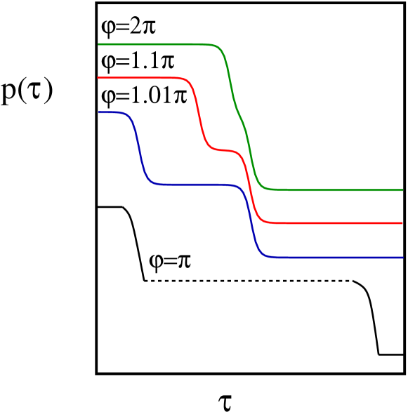
Figure 11: Instanton profile $p(\tau)$ for various values of $\varphi$. From top to bottom: $\varphi=2\pi,1.1\pi,1.01\pi,\pi$. The plots have been vertically shifted: in any case $p(\tau)$ ranges from 0 to 1. The dashed portion of the plot for $\varphi=\pi$ (black line) denotes infinite separation between the short instantons ($R\to\infty$).

Appendix C Tables of relevant integrals

In this appendix, we sketch the calculation of the integrals used in subsection 5.1 to compute $I_{\rm DC}(V)$ and $S(V)$ near by the WFP. All the relevant integrals may be recasted in the form

$$I_{\zeta}(z)=\int_{0}^{\infty}\>d\tau\>\frac{e^{-iz\tau}}{[e^{\frac{i\pi u}{L}\tau}-e^{-\frac{i\pi u}{L}(\tau-i\eta)}]^{\zeta}}\>\>\>\>,$$ (97)

with $\zeta$ real and $\eta=0^{+}$. To compute the integral, one assumes $z-\zeta\pi u/L<0$, and integrates over the closed integration path shown in Fig.12, to get

$$I_{\zeta}(z)=-i\int_{0}^{\infty}\>dw\>\frac{e^{-\left(\frac{\pi u\alpha}{L}+z\right)w}}{[e^{\frac{\pi u\eta}{L}}-e^{-\frac{2\pi w}{L}}]^{\zeta}}\>\>\>\>.$$ (98)

Figure 12: Integration path used to compute $I_{\zeta}(z)$ in Eq.(97)

The integral in Eq.(98) is tabulated [38], yielding

$$I_{\zeta}(z)=-i~{}_{2}F_{1}[\frac{Lz}{2\pi u}+\frac{\zeta}{2},\zeta,1+\frac{Lz}{2\pi u}+\frac{\zeta}{2};1]/[z-\frac{\zeta\pi u}{L}]\>\>\>\>,$$ (99)

where $~{}_{2}F_{1}$ is the confluent hypergeometric function. Then, using the identity

$$~{}_{2}F_{1}[a,b,c;1]=\frac{\Gamma[c]\Gamma[c-a-b]}{\Gamma[c-a]\Gamma[c-b]}\>\>\>\>,$$ (100)

in Eq.(99), one obtains Eqs.(50,51) of subsection 5.1. To analytically extend Eq.(99), one may use Stirling’s approximation, which yields

$$\Gamma[w]\approx\sqrt{2\pi}\>(w-1)^{w-\frac{1}{2}}\>e^{-(w-1)}\>\>\>\>.$$ (101)

Eq.(101) has been applied in subsection 5.1, when extracting the large-$L$ limit of $I_{\rm DC}(V)$ and of $S(V)$.

Appendix D Fermionization and exact solution of the BDSG model for $g=2$

In this appendix we carry out the fermionization procedure of $H_{\rm BDSG}=H_{\rm LL}+H_{\bf B}$ for $g=2$. As we will show, introducing a complete set of fermionic coordinates to represent the relevant fields of the model, allows for recasting $H_{\rm BDSG}$ in a quadratic form, thus making it exactly solvable. In the following, we assume $B_{\parallel}=0$ and, due to our interest in nonequilibrium dc transport properties, we resort to the real time formalism.

The fermionization of $H_{\rm BDSG}$ follows the same basic steps as in Ref.[36]. To begin with, one fermionizes $H_{\rm LL}$ for $g=2$ by writing $\Phi$ as the sum of two chiral fields, $\phi_{R},\phi_{L}$, as $\Phi(x,t)=\phi_{R}(x-ut)+\phi_{L}(x+ut)$. The chiral vertex operators $:e^{-i\phi_{R}(x-ut)}:$, $:e^{-i\phi_{L}(x+ut)}:$ may be the regarded as two chiral fermionic fields $\psi_{R},\psi_{L}$

$$\psi_{R}(x-ut)=\eta_{R}\frac{1}{\sqrt{L}}\>:e^{-i\phi_{R}(x-ut)}:\;\;\;,\;\;\psi_{L}(x+ut)=\eta_{L}\frac{1}{\sqrt{L}}\>:e^{-i\phi_{L}(x+ut)}:\>\>\>\>,$$ (102)

where $\eta_{R},\eta_{L}$ are the Klein factors, introduced to ensure the correct anticommutation relations between $\psi_{R}$ and $\psi_{L}$ [31].

To fermionize $H_{\bf B}$, one assumes Neumann BCs at both boundaries [36]; namely

$$\psi_{R}(0,t)=\psi_{L}(0,t)\;\;\;,\;\;\psi_{R}(L,t)=\psi_{L}(L,t)\>\>\>\>.$$ (103)

Eq.(103) is enforced if one uses [36] the noninteracting real time action for $\psi_{R},\psi_{L}$,

$$S_{0}^{\rm Fer}=i\>\int\>dt\>\int_{0}^{L}\>dx\>\left\{\psi_{R}^{\dagger}(0,t)\left[\frac{\partial}{\partial t}+u\frac{\partial}{\partial x}\right]\psi_{R}(0,t)+\psi_{L}^{\dagger}(0,t)\left[\frac{\partial}{\partial t}-u\frac{\partial}{\partial x}\right]\psi_{L}(0,t)\right\}$$

$$+i\frac{u}{2}\>\int\>dt\>\left\{\psi_{R}^{\dagger}(0,t)\psi_{L}(0,t)-\psi_{L}^{\dagger}(0,t)\psi_{R}(0,t)\right\}\>\>\>\>.$$ (104)

Then, one has to follow a different procedure for the term $\propto g_{1}$ and the term $\propto g_{2}$ in $H_{\bf B}$. Fermionizing the former, requires introducing additional local degrees of freedom $\xi,\xi^{\dagger}$, describing the spin-1/2 variable ${\bf S}$ emerging at C. Using a “rotated” Jordan-Wigner (JW) transformation [31], one introduces a complex fermion $\xi$, in terms of which ${\bf S}^{x},{\bf S}^{z}$ are given by

$${\bf S}^{x}\to\xi^{\dagger}\xi-\frac{1}{2}\;\;\;,\;\;{\bf S}^{z}\to\frac{\xi+\xi^{\dagger}}{2}\>\>\>\>.$$ (105)

Using Eqs.(102,105), and taking into account the boundary conditions in Eq.(103), one gets the contribution to boundary action which is $\propto g_{1}$; namely .

$$S_{B}^{(I)}=i\frac{g_{1}}{4}\>\int\>dt\>\{[\psi_{R}^{\dagger}(0,t)+\psi_{L}(0,t)]\xi-\xi^{\dagger}[\psi_{R}(0,t)+\psi_{L}^{\dagger}(0,t)]\}+i\int\>dt\>\xi^{\dagger}\frac{\partial\xi(t)}{\partial t}\>\>\>\>.$$ (106)

To fermionize the contribution to the boundary interaction which is proportional to $g_{2}$, one has to regularize, by point splitting, the products $:e^{ai\phi_{A}(0)}:\>:e^{bi\phi_{B}(0)}:$, with $a,b=\pm 1$ and $A,B=L,R$, and to require that the anticommutation relations between the chiral fermions are preserved. As a result, one gets

$$S_{B}^{(II)}=i\frac{g_{2}}{2}\int\>dt\>\left\{\psi_{R}^{\dagger}(0,t)\frac{\partial\psi_{L}^{\dagger}(0,t)}{\partial t}+\psi_{L}(0,t)\frac{\partial\psi_{R}(0,t)}{\partial t}\right\}$$

$$i\frac{g_{2}}{2}\int\>dt\>\left\{\psi_{R}^{\dagger}(0,t)\frac{\partial\psi_{R}(0,t)}{\partial t}+\psi_{L}^{\dagger}(0,t)\frac{\partial\psi_{L}(0,t)}{\partial t}\right\}\>\>\>\>.$$ (107)

Finally, the term $\propto B_{\perp}$ is fermionized using the JW transformation reported in Eq.(105) and, by adding the “kinetic” term for $\xi$, one gets the last contribution to the boundary action, which is given by

$$S_{B}^{(III)}=\int\>dt\>\left[i\xi^{\dagger}\dot{\xi}+2B_{\perp}\left(\xi^{\dagger}\xi-\frac{1}{2}\right)\right]\>\>\>\>.$$ (108)

From Eqs.(104,106,107,108), one sees that the full fermionic action is given by

$$S^{\rm Fer}=S_{0}^{\rm Fer}+S_{B}^{(I)}+S_{B}^{(II)}+S_{B}^{(III)}\>\>\>\>.$$ (109)

Equating to zero the functional derivative of $S^{\rm Fer}$, one obtains the boundary conditions for the fermionic fields, which are given by

$$-i\frac{u}{2}[\psi_{R}(0,t)-\psi_{L}(0,t)]+i\frac{g_{2}}{2}\left(\frac{\partial\psi_{L}^{\dagger}(0,t)}{\partial t}+\frac{\partial\psi_{R}(0,t)}{\partial t}\right)+i\frac{g_{1}}{2}\xi=0$$

$$i\dot{\xi}+B_{\perp}\xi-i\frac{g_{1}}{4}[\psi_{R}(0,t)+\psi_{L}^{\dagger}(0,t)]=0\>\>\>\>.$$ (110)

Getting rid of $\xi,\dot{\xi}$ in Eqs.(110) and using the normal mode expansion for $\psi_{R},\psi_{L}$, given by

$$\psi_{R}(x-ut)=\frac{1}{\sqrt{L}}\>\sum_{p}e^{i(x-ut)}\>\psi_{R}(p)\;\;\;,\;\;\psi_{L}(x+ut)=\frac{1}{\sqrt{L}}\>\sum_{p}e^{i(x+ut)}\>\psi_{L}(p)\;\;\;\;,$$ (111)

one eventually obtains the following linear relations between the normal modes $\psi_{R}(p),\psi_{L}(p)$

$$\psi_{R}(p) = R(p)\psi_{L}(-p)+Q(p)\psi_{L}^{\dagger}(p)$$

$$\psi_{R}^{\dagger}(-p) = Q(p)\psi_{L}(-p)+R(p)\psi_{L}^{\dagger}(p)\>\>\>\>,$$ (112)

with

$$R(p)=\frac{up+2B_{\perp}}{up+2B_{\perp}-i[-\frac{g_{1}^{2}}{8u}+ug_{2}p^{2}+2B_{\perp}g_{2}p]}\;\;\;\;,$$ (113)

and

$$Q(p)=\frac{i[-\frac{g_{1}^{2}}{8u}+ug_{2}p^{2}+2B_{\perp}g_{2}p]}{up+2B_{\perp}-i[-\frac{g_{1}^{2}}{8u}+ug_{2}p^{2}+2B_{\perp}g_{2}p]}\;\;\;\;.$$ (114)

Eqs.(113,114) provide the formulas we used in subsection 5.2 to compute $I_{\rm DC}(V)$ and $S(V)$ in the fermionized theory.

References

- [1] I. Affleck, Lecture Notes, Les Houches, 2008 (arXiv:0809.3474).
- [2] A. C. Hewson, “The Kondo Problem to Heavy Fermions”, Cambridge University Press (1997), and references therein.
- [3] P. Nozierès and A. Blandin, J. Phys.41,193 (1980); D. L. Cox and F. Zawadowski, Adv. Phys. 47, 599 (1998).
- [4] H. van Houten and C. W. J. Beenakker, Physics Today 49 (7), 22 (1996).
- [5] C. W. J. Beenakker and H. van Houten in ”Nanostructures and Mesoscopic Systems”, W. P. Kirk and M. A. Reed eds. (Academic, New York, 1992).
- [6] C. Chamon, M. Oshikawa and I. Affleck, Phys. Rev. Lett. 91, 206403(2003); M. Oshikawa, C. Chamon and I. Affleck, Journal of Statistical Mechanics JSTAT/2006/P02008.
- [7] D. Giuliano, P. Sodano, Nucl. Phys. B 811, 395 (2009)
- [8] J. Cardy, hep-th/0411189, Entry in Encyclopedia of Mathematical Physics, Elsevier (2006).
- [9] T. Giamarchi, “Quantum Physics in One Dimension”, (Oxford University Press, 2004).
- [10] L. I. Glazman and A. I. Larkin, Phys. Rev. Lett. 79, 3736 (1997).
- [11] D. Giuliano, P. Sodano, Nucl. Phys. B711, 480, (2005).
- [12] F.W.J. Hekking and L.I. Glazman, Phys. Rev. B 55, 6551 (1997).
- [13] D. Giuliano and P. Sodano, Nucl. Phy. B 770, 332 (2007).
- [14] A. M. Tsvelik and P. B. Wiegmann, Adv. Phys. 32, 453 (1983); P. Schlottmann, Phys. Rep. 181, 1 (1989); P. Nozieres and A. Blandin, J. Phys. (France), 41, 193 (1980); I. Affleck and A. W. Ludwig, Phys. Rev. B 48, 7297 (1993).
- [15] S. Eggert and I. Affleck, Phys. Rev. B 46, 10866 (1992).
- [16] P. Fendley. A. W. W. Ludwig, and H. Saleur, Phys. Rev. Lett. 74, 3005 (1995); A. M. Chang, Rev. Mod. Phys. 75, 1449 (2003).
- [17] See, for instance, A. O. Gogolin, A. A. Nersesyan, and A. M. Tsvelik, Bosonization and Strongly Correlated Systems, Cambridge University Press. (2004).
- [18] C.L. Kane and M. P. Fisher, Phys. Rev. Lett. 68, 1220 (1992); Phys. Rev. B46, 15233 (1992).
- [19] S. A. Reyes and A. M. Tsvelik, Phys. Rev. 95, (2005), 186404.
- [20] H.Yi and C.L.Kane, Phys.Rev.B 57,R5579-R5582(1998).
- [21] I. Affleck, M. Oshikawa and H. Saleur, Nucl. Phys. B594, 535 (2001).
- [22] J. Cardy, “Scaling and Renormalization in Statistical Physics”, Cambridge University Press, 1996.
- [23] R. Egger, A. Komnik, and H. Saleur, Phys. Rev. B 60, R5113 (1999).
- [24] P. Azaria, P. Lecheminant, and A. M. Tsvelik, arXiv:cond-mat/9806099.
- [25] A. Fendley, A. W. W. Ludwig, and H. Saleur, Phys. Rev. Lett.75, 2196 (1995); C. de Chamon, D. E. Freed, and X. G. Wen, Phys. Rev. B 51, 2363 (1995); A. Koutouza, H. Saleur, and B. Trauzettel, Phys. Rev. Lett. 91, 026801 (2003).
- [26] A. A. Kezhevnikov, R. J. Schoelkopf, and D. E. Prober, Phys. Rev. Lett. 84, 3398 (2000); K. E. Nagaev and M. Büttiker, Phys. Rev. B 63, 081301(R) (2001).
- [27] E. Sela, Y. Oreg, F. von Oppen, and J. Koch, Phys.Rev.Lett.97,86601(2006).
- [28] L. Saminadayar, D. C. Glattli, Y. Jin, and B. Etienne, Phys. Rev. Lett 79, 2526 (1997); R. de Picciotto, M. Reznikov, M. Heiblum, V. Umansky, G. Bunin, and D. Mahalu, Nature 389, 162 (1997).
- [29] F. Lefloch et al. Phys. Rev. Lett. 90, 067002 (2003).
- [30] O. Zarehin, M. Zaffalon, M. Heiblum, D. Mahalu, and V. Umansky, Phys. Rev. B 77, 241303 (2008).
- [31] For a review see, for instance, H. J. Shulz, G. Cuniberti and P. Pieri in Field Theories for Low-Dimensional Correlated Systems, G. Morandi, P. Sodano, V. Tognetti and A. Tagliacozzo eds., Springer, Berlin (2000).
- [32] D. K. Campbell, M. Peyrard, P. Sodano, Physica D 19, 165 (1986), and references therein.
- [33] E. Novais, A. H. Castro Neto, L. Borda, I. Affleck, and G. Zarand, Phys. Rev. B 72, , 014417 (2005).
- [34] D. Giuliano and P. Sodano, New. Jour. of Physics 10,093023(2008).
- [35] D. Giuliano and P. Sodano, EPL 88, 17012 (2009).
- [36] M. Ameduri, R. Konik, and A. LeClair, Phys. Lett. B 354, 376 (1995).
- [37] See, for example, P. Ginsparg, “Applied Conformal Field Theory”, in Field, Strings and Critical Phenomena, Les Houches, Section XLIX, (1988), Edited by E. Brézin and P. Zinn-Justin; J. Cardy, “Conformal invariance and statistical mechanics”, ibidem.
- [38] M. Abramowitz and I. A. Stegun, Handbook of Mathematical Functions, (United States. National Bureau of Standards. Applied mathematics series, 55, 1964).