Magnetomotive drive and detection of clamped-clamped mechanical resonators in water

Abstract

We demonstrate magnetomotive drive and detection of doubly clamped string resonators in water. A compact 1.9 T permanent magnet is used to detect the fundamental and higher flexural modes of $\mathrm{200\,\mu m}$ long resonators. Good agreement is found between the magnetomotive measurements and optical measurements performed on the same resonator. The magnetomotive detection scheme can be used to simultaneously drive and detect multiple sensors or scanning probes in viscous fluids without alignment of detector beams.

Micro- and nanomechanical resonators have many applications as scanning probes and mass or stress sensors. Several techniques have been developed to detect resonator vibrations in vacuum and at atmospheric pressure. The natural environment for biological experiments however is an aqueous solution, and detection methods in liquid environments are less numerous. Optical or piezoresistive schemes are commonly used, combined with a separate excitation source, e.g. magnetic Vančura et al. (2005) or piezoelectric, to drive the strongly damped resonator.
In this work we demonstrate that a magnetomotive technique can be used to drive and detect micromechanical resonator vibrations in water. The magnetomotive technique allows straightforward resonator geometry, a strong driving force acting directly on the resonator, and it can be scaled towards nanometer dimensions. The technique has been applied in vacuum to characterize resonators up to the $\mathrm{GHz}$-range  Huang et al. (2003), in mass sensing Huang et al. (2005), and to readout resonator arrays driven in the nonlinear regime at atmospheric pressure Venstra and van der Zant (2008).

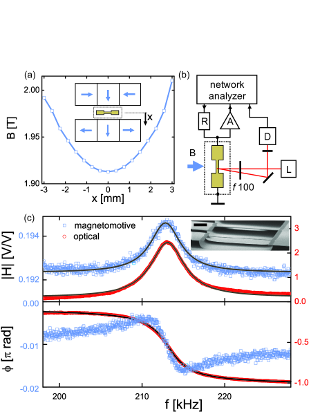
Figure 1: (a) Magnetic field strength as a function of the position in the gap between the magnet poles, $x$. Inset shows a cross-section of the magnet construction, squares represent the individual magnets, polarized according to the arrows. (b) Schematic of the combined magnetomotive and optical setup. (c) Frequency response functions of the magnetomotive driven resonator in air, as measured by magnetomotive and optical techniques, magnitude $\mathrm{|H|}$ and phase $\mathrm{\phi}$, the black solid lines represent driven harmonic oscillator functions fits. Inset: scanning electron micrograph of two clamped-clamped string resonators, scale bar is $\mathrm{20\,\mu m}$.

A compact and powerful permanent magnet is constructed to drive the strongly damped resonator in the fluid. The magnet is composed of commercially available NdFeB magnets with a remanent induction of $\mathrm{B_{r}=1.5\,T}$ and a total volume of $\mathrm{213\,cm^{3}}$. By configuring the magnets in a Halbach array Halbach (1983), a field strength up to $\mathrm{2\,T}$ is generated in a $\mathrm{6\,mm}$ gap between the magnet poles. Figure 1(a) shows the measured field as a function of the position in the gap, $x$. The inset shows a schematized cross section of the construction, the arrows indicate the polarization of the magnets. The field strength varies less than $5\%$ within a volume of $\mathrm{6\times 6\times 6\,mm^{3}}$ inside the gap, and is minimum in the center at $x\,\mathrm{=0}$, where the resonator is located.
Figure 1(b) shows the measurement setup. The alternating voltage from a network analyzer is applied to the resonator via a series resistor, ${\mathrm{R=25\,\Omega}}$. The generated electromotive force is measured via a high impedance buffer, marked A in the figure, on one input channel of the analyzer. As a reference, the deflection of the resonator is probed at the same time by a Helium Neon laser, L. The beam reflection is captured on a linear position sensitive detector, D, and measured on the second input channel of the network analyzer.
The resonator is placed in a custom-built temperature controlled flow cell with a volume of $\mathrm{3\,\mu l}$, such that the Lorentz force is directed out-of-plane, corresponding to the fundamental resonance mode.
The resonators are fabricated from $\mathrm{100\,nm}$ thick low-pressure chemical vapor deposited silicon nitride using electron beam lithography and reactive ion etching, and suspended using a dry isotropic release process. The inset in Fig. 1(c) shows two resonators before metallization. The dimensions are $L\times w=\mathrm{200\times 15\,\mu m^{2}}$. A $\mathrm{5\,nm}$ thick chromium adhesion layer is deposited on top, followed by $\mathrm{30\,nm}$ of gold. The gold layer is not passivated and is in contact with the water during the experiments.
In air, the fundamental resonance mode, measured by the magnetomotive and optical techniques is shown in Fig.1(c). The signal to noise ratio for the optical measurement is $\mathrm{50}$ times larger, which is due to the approximately $200$ times amplification of the resonator displacement by the optical lever. The resonator resistance, $\mathrm{R\approx 7.5\,\Omega}$, is large compared to its motional impedance, $\mathrm{Z_{0}\approx 0.8\,\Omega}$ at resonance, and this results in a phase response for the magnetomotive measurement different from the driven harmonic oscillator response obtained by the optical detector. By fitting damped driven harmonic oscillator functions represented by the solid black lines, the natural (undamped) resonance frequency for the fundamental mode is $f_{\mathrm{1,air}}\mathrm{=213\,kHz}$, and the quality factor $Q_{\mathrm{1,air}}=50$. The magnetomotive technique can be applied to higher odd modes, though the sensitivity reduces, as will be discussed later. The third resonance mode is also measured with $f_{\mathrm{3,air}}\mathrm{=725\,kHz}$. For the n-th mode of vibration, the frequency ratio $f_{\mathrm{n}}/f_{\mathrm{1}}=n$ for a string in tension, and roughly $(\frac{2n+1}{3})^{2}$ for a doubly clamped flexural beam Weaver et al. (1990). The measured ratio $f_{\mathrm{3,air}}/f_{\mathrm{3,air}}=3.4$, indicates string-like behavior dominates. This occurs when the restoring force from flexure is small compared to that from residual tension. We note that the ratio is $\mathrm{13\%}$ larger than for a string in tension, and this is explained by the flexural rigidity which contributes to some increase in effective spring stiffness, whereas the compliance from the large undercuts decreases it slightly.

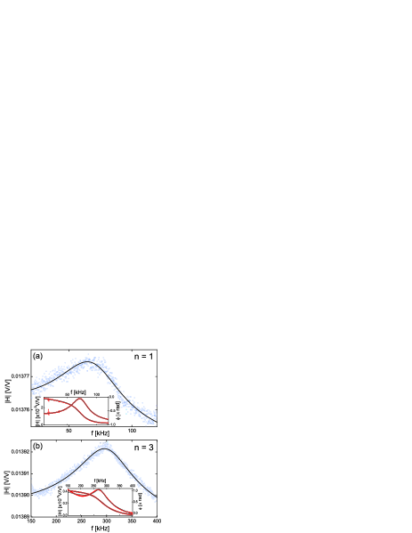
Figure 2: (a) Magnetomotive measurement of the fundamental resonance mode of the string resonator in water. The inset shows the optical measurement. (b) Magnetomotive and optical measurement of the third flexural mode.

Prior to experiments in water, the flow cell is flushed with ethanol to remove air bubbles. De-ionized water is injected and the optical and magnetomotive measurements are repeated on an immersed resonator. Figure 2(a) shows the measured amplitude response using the magnetomotive scheme for the first resonance mode. A harmonic oscillator function is fit through the data with $f_{\mathrm{1,water}}\mathrm{=74\,kHz}$, which is identified as a mechanical resonance by the magnitude and phase response from the optical measurement, shown in the inset. A different Q-factor is found for the magnetomotive and optical detector. The magnetomotive quality factor, $Q_{\mathrm{1,water}}\mathrm{=1.4}$ is lower than for the optical measurement $Q_{\mathrm{1,water}}\mathrm{=2.8}$. This difference is attributed to the complex dielectric constant of water, which presents a frequency-dependent load to the resonator and lowers the Q-factor for the magnetomotive measurement Cleland and Roukes (1999). The value of the load depends on the design of sample and flow cell and on the frequency-dependent dielectric properties of water, and is not further discussed here.
The third flexural mode of the same resonator is plotted in Fig. 2(b). The magnetomotive detected resonance frequency equals $f_{\mathrm{3,water}}\mathrm{=306\,kHz}$ and $Q_{\mathrm{3,water}}=2.7$. The optical measurement reveals a slightly lower resonance frequency, $f_{\mathrm{3,water}}\mathrm{=275\,kHz}$. This difference was found independent on sweep time and driving strength, and cannot be explained by electrical loading of the resonator. The optically measured Q-factor equals $Q_{\mathrm{3,water}}=6.4$, again higher than the magnetomotive one. In water the ratio between the resonance frequencies is similar to the ratio in air: $f_{\mathrm{3,water}}/f_{\mathrm{1,water}}=3.8$.
To compare the shift in resonance frequency and Q-factor upon immersion with theory, we take the viscous and inertial forces into account through a hydrodynamic function, $\Gamma(\mathrm{Re,\kappa})$, which relates the cross section shape of the resonator to a force per unit length acting on the resonator, where its real and imaginary components correspond to the inertial and dissipative components of the force Sader (1998). $\Gamma(\mathrm{Re,\kappa)}$ is a function of the normalized mode-dependent Reynolds number, $\mathrm{Re_{n}}=2\pi f_{\mathrm{n,vac}}\rho/\eta$, and the normalized mode number, $\mathrm{\kappa_{n}=\pi n\frac{w}{L}}$ for our string resonators. Here $\mathrm{\rho}$ is the density and $\mathrm{\eta}$ the dynamic viscosity of water. The hydrodynamic function for a rectangular cross section is given in Ref. Van Eysden and Sader (2007), and we can calculate the ratio between the frequencies:

$$\frac{f_{\mathrm{n,water}}}{f_{\mathrm{n,vac}}}=[1+\frac{\pi w\rho}{4t\rho_{\mathrm{c}}}\Gamma_{\mathrm{R}}(\mathrm{Re,\kappa)}]^{-0.5},$$ (1)

where $\rho_{\mathrm{c}}$ denotes the average density of the gold coated resonator, $\mathrm{\Gamma_{R}}$ denotes the real part of $\Gamma(\mathrm{Re,\kappa})$, and $\mathrm{\pi w\rho/4t\rho_{c}}$ represents the mass loading parameter Villa and Paul (2009). Although this model assumes a high Q–factor, experiments have shown it accurately describes the response of cantilever beams with Q–factors close to ours Chon and Sader (2000). The results for the resonance frequencies and Q-factors are summarized in Table 1. We measured the resonance frequency from thermal noise spectra in atmospheric pressure and in the intrinsic damping regime in vacuum, and found $f_{\mathrm{1,air}}/f_{\mathrm{1,vac}}=1.013$ and $f_{\mathrm{3,air}}/f_{\mathrm{3,vac}}=1.007$, which is negligible compared to the shifts upon immersion in water Qai . We can thus assume $f_{\mathrm{n,air}}=f_{\mathrm{n,vac}}$, and the observed ratio’s $f_{\mathrm{n,water}}/f_{\mathrm{n,vac}}$ are close to the theoretical prediction. The slightly higher prediction of the resonance frequency and Q-factors may be explained by the limited distance between the resonator and the substrate. In our experiment the distance is comparable to the resonator width, and in this case additional friction reduces the Q-factor by a factor of 2 when compared to a freely moving resonator Gittes and Schmidt (1998).

Table 1: Resonance frequency and Q-factor of mode $n$ in air and water, measured on a second device. The theoretic and experimental ratio’s between the resonance frequencies upon immersion are $r_{\mathrm{theory}}=f_{\mathrm{water}}/f_{\mathrm{vac}}$ and $r_{\mathrm{exp}}=f_{\mathrm{water}}/f_{\mathrm{air}}$.

	frequency (kHz)					$\mathrm{Q-factor}$
n		air	water	$r_{\mathrm{theory}}$	$r_{\mathrm{exp}}$		air	water	water,theory
1		194.9	52.6	0.23	0.27		50	2.0	4.1
3		593.3	184	0.25	0.31		67	5.4	6.7

To investigate the possibility to scale-down the dimensions of the string resonators, we have calculated the displacements and electromotive voltages at resonance Yurke et al. (1995). In the harmonic regime, the tension force $T$ is constant and sufficient to ensure string-like behavior with mode shapes and amplitudes $\mathrm{N_{n}}$ given by $\mathrm{u_{n}(x)=N_{n}\sin(\pi nx/L)}$. The maximum displacement of the string for $\mathrm{n}=1,3,..$, can then be calculated as der :

$$u_{\mathrm{max,n}}=\frac{4BIQ_{n}L^{2}}{n^{3}\pi^{3}T}$$ (2)

with $\mathrm{B}$ the magnetic field and $I$ the current through the resonator. For currents in the mA-range and an estimated residual stress of $\mathrm{60\,MPa}$, the amplitude at resonance is about $\mathrm{u_{max,1}=10\,nm}$ for the first mode, and decreases with the mode number cubed. We note that the excellent thermalization in water allows large drive currents without damaging the resonator, and large resonator amplitudes can be obtained. The generated electromotive voltage is given by

$$V_{\mathrm{EMF,n}}=\frac{8}{\pi^{3}}\frac{f_{n}IB^{2}Q_{n}L^{3}}{n^{3}T}$$ (3)

for odd mode numbers. For even $n$, the net flux rate is zero and no voltage is generated. The resonance frequency $f_{\mathrm{n}}$ scales with the inverse dimension ($d^{-1}$). Furthermore, in these experiments the tension force, $\mathrm{T}$, results from residual stress and therefore scales as ($wt=d^{2}$). In a harmonic spectrum, $f_{\mathrm{n}}=\mathrm{n}f_{\mathrm{1}}$, the generated voltage is thus independent on the mode number and proportional to the displacement $u_{\mathrm{n,max}}$, which is adjustable by the driving force. Therefore $V_{\mathrm{EMF}}\sim fL^{3}/T\sim d^{0}$, independent on dimension.

Figure 3: Temperature dependence of the resonance frequency (a) and Q-factor (b) of the fundamental resonance mode of an immersed string resonator.

Changes in liquid density and viscosity associated with temperature fluctuations pose a limit on the stability and accuracy of frequency-based measurements. Electrical and mechanical energy is dissipated by the strongly driven resonators (i.e. by ohmic resistance and by the viscous force), and an increase of water temperature is the result. The electrical and mechanical dissipation can be expressed as $U_{\mathrm{in}}=I^{2}R+2\pi^{2}mf^{3}_{n}u_{max}^{2}/Q$. In our experiments the contributions are on the order of $\mathrm{U_{in,e}=10^{-5}\,J/s}$ for the electrical and $\mathrm{U_{in,m}=10^{-12}\,J/s}$ for the mechanical dissipation, and electrical dissipation is dominant. If we apply the input energy to heat the $\mathrm{3\,\mu l}$ volume of water inside the flow cell, a temperature increase on the order of $\mathrm{60\,mK/s}$ is the result. We investigated the effect of such temperature fluctuations by measuring the resonance frequency and Q-factor during a controlled temperature sweep over a range of $\mathrm{20\,^{o}C}$. As shown in Fig. 3, both the resonance frequency and the Q-factor increase while increasing the temperature, as expected due to the reduction of the fluid density and viscosity. The results presented here for doubly clamped string resonators are comparable to results obtained earlier for cantilever beams Kim and Kihm (2006). The temperature dependence of the resonance frequency, approximately $\mathrm{100\,Hz/^{o}C}$ in this experiment, underlines the need for accurate temperature control during mass sensing experiments in liquids.
In summary, we demonstrated magnetomotive drive and detection of micromechanical string resonators in water. The fundamental and third flexural resonance modes were detected, and the observed changes in resonance frequency and Q-factor are in agreement with theory. The magnetomotive technique can be applied to obtain large vibration amplitudes in water, and to detect the resonator motion without alignment of probe beams, as with optical detection schemes. Higher modes can be used to enhance sensitivity, and to measure the mass of single particles regardless of the location of the accretion on the resonator surface Dohn et al. (2006).
The authors acknowledge financial support from the Dutch organizations FOM and NWO (VICI), and Koninklijke Philips NV (RWC-061-JR-05028).

References

- Vančura et al. (2005) C. Vančura, J. Lichtenberg, A. Hierlemann, and F. Josse, Appl. Phys. Lett. 87, 162510 (2005).
- Huang et al. (2003) X. M. H. Huang, C. A. Zorman, M. Mehregany, and M. L. Roukes, Nature 421, 496 (2003).
- Huang et al. (2005) X. M. H. Huang, M. Manolidis, S. C. Jun, and J. Hone, Appl. Phys. Lett. 86, 143104 (2005).
- Venstra and van der Zant (2008) W. J. Venstra and H. S. J. van der Zant, Appl. Phys. Lett. 93, 234106 (2008).
- Halbach (1983) K. Halbach, IEEE Trans. Nucl. Sci. NS-30, 3323 (1983).
- Weaver et al. (1990) W. Weaver, S. P. Timoshenko, and D. H. Young, Vibration Problems in Engineering, edition (Wiley-Interscience, 1990).
- Cleland and Roukes (1999) A. N. Cleland and M. L. Roukes, Sensor Actuat A 72, 265 (1999).
- Sader (1998) J. E. Sader, J. Appl. Phys. 84 (1998).
- Van Eysden and Sader (2007) C. A. Van Eysden and J. E. Sader, J. Appl. Phys. 101 (2007).
- Villa and Paul (2009) M. M. Villa and M. R. Paul, Phys. Rev. E 79 (2009).
- Chon and Sader (2000) P. Chon, J W M Mulvaney and J. E. Sader, J. Appl. Phys. 87 (2000).
- (12) The ratio’s of the Q-factors are and .
- Gittes and Schmidt (1998) F. Gittes and C. F. Schmidt, Eur. Biophys. J. 27, 75 81 (1998).
- Yurke et al. (1995) B. Yurke, D. S. Greywall, A. N. Pargellis, and P. A. Busch, Phys. Rev. A 51, 4211 (1995).
- (15) For the tension dominated regime , where the modeshapes are given by .
- Kim and Kihm (2006) S. Kim and K. D. Kihm, Appl. Phys. Lett. 89, 061918 (2006).
- Dohn et al. (2006) S. Dohn, O. Hansen, and A. Boisen, Appl. Phys. Lett. 88, 264104 (2006).