X-Ray Measured Dynamics of Tycho’s Supernova Remnant

Abstract

We present X-ray proper-motion measurements of the forward shock and reverse-shocked ejecta in Tycho’s supernova remnant, based on three sets of archival Chandra data taken in 2000, 2003, and 2007. We find that the proper motion of the edge of the remnant (i.e., the forward shock and protruding ejecta knots) varies from 0^′′.20 yr^-1 (expansion index $m=0.33$, where $R=t^{m}$) to 0^′′.40 yr^-1 ($m=0.65$) with azimuthal angle in 2000-2007 measurements, and 0^′′.14 yr^-1 ($m=0.26$) to 0^′′.40 yr^-1 ($m=0.65$) in 2003-2007 measurements. The azimuthal variation of the proper motion and the average expansion index of $\sim$0.5 are consistent with those derived from radio observations. We also find proper motion and expansion index of the reverse-shocked ejecta to be 0^′′.21–0^′′.31 yr^-1 and 0.43–0.64, respectively. From a comparison of the measured $m$-value with Type Ia supernova evolutionary models, we find a pre-shock ambient density around the remnant of $\lesssim 0.2$ cm^-3.

1. Introduction

A supernova (SN) event which Danish astronomer Tycho Brahe discovered in 1572 is now visible at many wavelengths as Tycho’s SN remnant (SNR). The SN event has been classified as a normal Type Ia (i.e., a thermonuclear explosion of a white dwarf star in a close binary) based on the shape of its light curve (e.g., Baade 1945; Ruiz-Lapuente 2004) and the X-ray properties (Badenes et al. 2006). This is recently confirmed from its light-echo spectrum, which reached the earth about 436 yr after Tycho Brahe observed the direct light from the SN event (Krause et al. 2008). Given the fact that Type Ia SNe have been used to determine cosmological parameters such as the Hubble constant and the Dark Energy equation of state (e.g., Hamuy et al. 1996; Riess et al. 1998), it is fundamentally important to understand the explosion mechanism and the progenitor system. Tycho’s SNR is a very suitable target for such a study. First, its ejecta-dominated X-ray emission allows us to constrain the explosion mechanism models as was recently demonstrated by Badenes et al. (2006), who concluded that the explosion producing Tycho’s SNR was most likely a delayed detonation; also, the surviving binary companion from Tycho’s SNR may have been identified (Ruiz-Lapuente et al. 2004; Ihara et al. 2007), though the association with the SN event is still controversial (Kerzendorf et al. 2009). The chemical abundances of the candidate companion were recently measured to be consistent with the Galactic trend except for an overabundant Ni/Fe ratio which suggests contamination by SN ejecta (Hernandez et al. 2009). Recent detection of Cr and Mn K$\alpha$ lines in the X-ray spectrum of the SNR (Tamagawa et al. 2009; Yang et al. 2009) also provides an opportunity to constrain the metallicity of the progenitor star (Badenes, Bravo, & Hughes 2008).

Another important aspect of Tycho’s SNR is the presence of non-thermal X-ray synchrotron emission produced by accelerated particles (e.g., Pravdo & Smith 1979). Recent Chandra images have revealed that the non-thermal emission is confined to a very thin shell just behind the forward shock (Hwang et al. 2002; Bamba et al. 2005; Warren et al. 2005). The thin filamentary structure of non-thermal emission is now known to be a common feature in many young SNRs, while its nature is the subject of considerable theoretical work on particle acceleration (e.g., Pohl et al. 2005; Ballet 2006; Cassam-Chenaï et al. 2007). Furthermore, this SNR is a possible TeV gamma-ray source, although a firm detection of TeV gamma-ray emission is not yet available (e.g., Völk et al. 2008).

Tycho’s SNR potentially provides us with information on SNR evolution, since the degree of deceleration of the forward shock can be inferred by combining the current expansion rate with the accurately known age. Expansion measurements have been performed at optical, radio, and X-ray wavelengths. Optical measurements have focused on the northwestern (NW), northern (N), and eastern (E) H$\alpha$ filaments. The expansion index ($m$; $R\varpropto t^{m}$, where $R$ and $t$ are the radius and the age of the remnant) for these filaments was measured to be 0.32–0.41 (Kamper & van den Bergh 1978), indicating significant deceleration from free expansion ($m=1$). The radio observations revealed that the expansion index varies between 0.2 and 0.8 with azimuthal angle (e.g., Reynoso et al. 1997). The slow expansion ($m\sim 0.2$) seen at the E rim suggests an interaction between the forward shock and a dense cold cloud. Such an interaction was confirmed by the subsequent discovery of a dense cloud toward the E rim (Reynoso et al. 1999; Lee et al. 2004). The mean $m$ value was calculated to be $\sim$0.47, suggesting that overall, this SNR is still evolving toward the Sedov phase ($m=0.4$). Although the mean value of $m$ for radio observations is higher than that for optical observations, optical and radio measurements of individual features are consistent with each other. In X-rays, the only X-ray expansion measurement to date was performed using ROSAT data with moderate angular resolution of $\sim$8^′′ half-power diameter (Hughes 2000). Interior features of the remnant show consistent expansion indices between X-ray and radio observations. In contrast, the expansion index for the forward shock measured in X-rays, $m\sim 0.71$, is higher than that for radio. Since the radio and X-ray images are well correlated with each other, the expansion rate discrepancy has been puzzling.

Here, we present X-ray proper-motion measurements based on archival Chandra data with superior angular resolution of $\sim$0.5^′′ half-power diameter taken in three epochs between 2000 and 2007. These Chandra data allow us to measure proper motions of the SNR edges as well as the reverse-shocked ejecta inside the remnant.

2. Observations and Data Reduction

Chandra observed Tycho’s SNR in three epochs as summarized in table 1. The third epoch comprises two observations taken on April 23 and 26 in 2007 (ObsID 7639 and 8551; PI: Hughes). The exposure time of ObsID 8551 was significantly shorter than that of ObsID 7639. For simplicity, we use only the longer observation (ObsID 7639) in our analysis. The information of the Chandra observations used in this paper is listed in. The time differences between the first and the third observations (i.e., 2000-2007) and between the second and the third (i.e., 2003-2007) are 6.60 yr and 3.99 yr, respectively. The observations in 2003 and 2007 were specifically intended to allow proper-motion measurements: both have the same pointing direction, roll angle, and exposure time. The Advanced CCD Imaging Spectrometer (ACIS)-I was used for these two observations. On the other hand, the 2000 observation was not intended for this purpose, and utilized the back-illuminated ACIS-S3 detector. However, the 2000 observation is still useful to measure proper motions. Therefore, we use the 2000 observation, which in fact provides slightly tighter constraints on proper motion due to the longer interval between observations. We reprocessed all the level-1 event data, applying the standard data reduction with CALDB ver. 3.4.0. The net exposure times for the 2000, 2003, and 2007 observations are 48.9 ks, 145.7 ks, and 108.9 ks, respectively. In order to make use of the best position accuracy of the ACIS, we removed the effects of pixel randomization.

Figure 1 shows a three-color Chandra image obtained from the 2003 observation. Red corresponds to low-energy (0.3–1.0 keV, mostly Fe L), green to middle-energy (1.0–4.0 keV, mostly Si+S+Ar+Ca K), and blue to high-energy (4.0–8.0 keV, mostly Fe K blend plus the continuum) bands. The remnant is outlined by thin blue (nonthermally-dominated) filaments, while it contains substantial green (thermally-dominated) fragmentation inside the blue filaments. The blue filaments are identified as the forward shock (e.g., Warren et al. 2005), while the fragments are the reverse-shocked ejecta (e.g., Velazquez et al. 1998). We measure proper motion of both the forward shock and the shocked ejecta, by comparing vignetting-corrected 1.0–8.0 keV images obtained in the three epoches.

3. Proper Motion Measurements

Before measuring proper motions, we try to register the three images by aligning the positions of several obvious X-ray point sources surrounding the remnant. We determine their positions in each epoch, by employing wavdetect software included in CIAO ver. 4.0. We detect nine sources around the SNR in the 2003 and 2007 images, while only five are detected along the NW periphery in the 2000 image. The smaller number of sources in the 2000 image is partly due to the fact that the southern portion of the SNR was not covered by ACIS-S3 chip, and partly due to the shorter exposure time. If we align only the sources concentrated in the small NW area, it may cause misalignment for the rest of the image. Therefore, we do not correct the registration between the 2000 and 2007 observations, and instead incorporate into our proper motion measurement for 2000-2007 a systematic uncertainty of 0^′′.4, which is the 1-sigma absolute astrometric accuracy for the ACIS camera reported by the Chandra calibration team. This systematic uncertainty seems to be conservative, because the rms residual calculated for the five point sources detected in both images is only 0^′′.13. On the other hand, we use the point sources to register images between 2003 and 2007. Since no optical counterpart was identified within a 1^′′ radius for any of the point sources based on any catalogs contained in the VizieR catalog service, we assume that none have undergone proper motion between 2003 and 2007. We aligned the coordinates of the images so that the point sources have the same positions, by using ccmap and ccsetwcs in IRAF IMCOORDS. In the alignment procedure, four parameters for the second-epoch image are allowed to vary: x and y shifts, rotation, and pixel scale. The best-fit parameters show differences for both x and y shifts of less than 0^′′.2, no modifications of pixel scales, and rotation of $3^{\prime}$, respectively. After the alignment, the rms residual for the positions of the nine point sources between 2003 and 2007 images is $\sim$0^′′.29, which will be taken as the systematic uncertainty in our proper-motion measurements for 2003-2007.

Figure 2 left and right show the difference images in the 1.0–8.0 keV energy band for 2000-2007 and 2003-2007, respectively. The subtraction is performed after each image was registered and smoothed by a Gaussian kernel of $\sigma=0^{\prime\prime}$.492 (i.e., 1 ACIS pixel) which is approximately the angular resolution of Chandra’s X-ray telescope. There are some artifacts in the difference images: the southern dark (negative) region seen in the 2000-2007 difference image which is due to the fact that the 2000 image has no exposure there, the structures running from NW to SE and from NE to SW caused by the ACIS chip gaps, and stripes running from NE to SW caused by bad columns. Apart from these artifacts, we can clearly see motion of the X-ray features as adjacent black and white features for the forward shock (the edge of the remnant) and the reverse-shocked ejecta (knotty features inside the remnant). We quantify the proper motion of these features in the following sections.

3.1. SNR Edges

3.1.1 Forward Shock

In order to measure proper motions accurately for the forward shock, we generate one-dimensional X-ray profiles along the apparent direction of shock motions, following Katsuda, Tsunemi, & Mori (2008). These one-dimensional X-ray profiles are extracted from the 39 small boxes (25${}^{\prime\prime}\times$25^′′) indicated in Fig. 1. The position angle of each box is chosen such that it is as perpendicular as possible to the shock front (by eye). The choice of position angle does not affect the proper motion measurement within at least $\pm 6$ degrees difference, which we checked for several boxes. In order to include the calibration uncertainty of the ACIS effective area, we add a 5 systematic error term in quadrature to the statistical error for each data point. Each profile is binned by 0^′′.5 along the radial direction of the SNR. An example profile is shown in Fig. 3, in which the shift due the motion of the shock is readily apparent. Shifting the first-epoch profile and calculating the $\chi^{2}$ values from the difference between the two profiles at each shift position, we search for the best-matched shift position for each box. Figure 4 shows the $\chi^{2}$ distribution as a function of shift position for the example profiles in Fig. 3. By applying a quadratic function for the $\chi^{2}$ profile, we measure the best-shift position where the minimum $\chi^{2}$ value occurs. In this way, we obtain two (2000-2007 and 2003-2007) results for each box. The reduced-$\chi^{2}$ value, which is nearly equal to $\chi^{2}$ value divided by the number of bins in each box (here 36), falls in the ranges 0.9–10.4 for 2000-2007 and 0.9–2.6 for 2003-2007 at the best-matched shift positions. Two neighboring boxes (azimuth angles = 78^∘ and 85^∘ counterclockwise from N) for the 2000-2007 measurements have large ($>$3.7) reduced-$\chi^{2}$ values. This is partly due to the fact that these two include the brightest parts among the entire SNR edge, resulting in smaller statistical errors than those of the others, and partly due to the fact that the angular resolution around the two boxes are significantly different between 2000 and 2007 observations. At the location of the two boxes, we simulate point spread functions (PSFs) for 2000 and 2007 images by using chart and marx software, and find that the shape of the PSF for the 2000 image is elongated in the direction of shock motion, while that for the 2007 image is not. If we fit the PSFs with a Gaussian kernel, we obtain $\sigma\sim 1^{\prime\prime}.7$ and $\sigma\sim 0^{\prime\prime}.9$ for the 2000 and 2007 images, respectively. Therefore, we smooth the 2007 image by a Gaussian kernel of $\sigma=1^{\prime\prime}.476$ (i.e., 3 ACIS pixels), such that it has the same image resolution as that of the 2000 image. In this way, we obtained reasonable fits for all the box regions (reduced-$\chi^{2}<$ 2.6).

Also notable in Fig. 3 is possible flux variations among the three epochs. We find that X-ray flux variations among the three epochs are within $\sim$10% for all the boxes. The 10% flux changes are larger than the ACIS effective area calibration uncertainty (5%). Considering that the magnetic field strength in Tycho’s SNR is thought to be in the milligauss range (e.g., 0.1–10 mG, Reynolds & Ellison 1992; 0.03–0.4 mG, Warren et al. 2005), year-scale flux variations of the synchrotron emission seen in RXJ11713.7$-$3946 (Uchiyama et al. 2007) or Cas A SNRs (Uchiyama & Aharonian 2008) may be expected in Tycho’s SNR as well. However, the possible flux variations in Tycho’s SNR are small compared with those seen in these other SNRs, where some knots showed more than 100% flux variations. Further detailed investigations are needed to determine whether the flux variation is due to the flux change of the synchrotron emission, and is beyond the scope of this paper.

3.1.2 Ejecta Knots Protruding beyond the Forward Shock

There are breakout regions along the periphery of the SNR, as indicated by the small annular segments with triangular marks in Fig. 1. In these regions, the SNR edges show fragmented features which look like Rayleigh-Taylor fingers. It is already shown that this fragmentation is formed by ejecta knots protruding beyond the forward shock, based on spectral analysis of XMM-Newton data (Decourchelle et al. 2001) as well as principal component analysis of Chandra data (Warren et al. 2005). Since these ejecta knots show completely different morphology from the filamentary structure of the forward shock, we cannot define box regions relative to the shock front. We thus use two-dimensional images instead of one-dimensional profiles to measure the proper motion. We follow the method employed by DeLaney & Rudnick (2003), who measured proper motion of the forward shock in Cas A. We first generate polar-coordinate images for the three observations. Then, radially shifting the polar-coordinate image from 2000 or 2003 by steps of 0^′′.5 with respect to 2007 image, we search for the best-matched shift positions. To quantitatively obtain the best-shift position, we calculated the $C$ value at each shift position, where $C$ is expressed as (Cash 1979; Vink 2008),

$$C=-2\mathrm{ln}P=-2\sum_{i}(n_{i}\mathrm{ln}m_{i}-m_{i}-\mathrm{ln}n_{i}!),$$

with $n_{i}$ being the observed counts in a pixel $i$ and $m_{i}$ being the model counts in the same pixel. We here assume that the 2007 observation is the model image. Using the $C$ value rather than $\chi^{2}$ is necessary when the number of counts is so low that the shape of the Poisson distribution becomes significantly different from that of the Gaussian distribution. In fact, this is the case for a number of pixels in the data used here. Since the analyzed areas (i.e., the small annular segments in the Fig. 1) include regions outside the remnant, they contain a significant number of pixels with zero counts. Although we cannot sum pixels with $n_{i}$ (or $m_{i}$) = 0 according to the above equation, we have to sum the same numbers of pixels for each shift position. To this end, we assume the observed and model counts in the pixels having zero counts to be unity. We check the validity of this assumption, by applying the two-dimensional method for several forward shock regions and confirming that the proper motion value obtained from the one- and two-dimensional methods are consistent with each other. As an example, the $C$ values calculated for the yellow box in Fig. 1 is shown as a function of shift position in Fig. 4 (with dashed lines), from which we can see that the best-shift position from the two-dimensional method ($C$ value) is the same as that from the one-dimensional method ($\chi^{2}$ value). The best-shift position for each area is estimated by fitting a quadratic function for each profile. In estimating uncertainties, $\Delta C$ (= $C_{\mathrm{min}}-C$) can be treated as $\Delta\chi^{2}$ (Cash 1979). In this way, we obtained two sets (2000-2007 and 2003-2007) of proper motion measurements for each small annular segment.

3.1.3 Results for the SNR Edge

Table 2 gives the proper motion, expansion rate, and expansion index (which are derived from “the expansion rate” $\times$ “the age of the remnant, i.e., 430 or 432 yr for 2000-2007 or 2003-2007, respectively”) for all areas including the forward shock (small boxes in Fig. 1) and ejecta knots (small annular pieces in Fig. 1). We also list the mean values which are simply the sum for all areas (both 2000-2007 and 2003-2007 measurements) divided by the number of areas. To calculate the expansion rate and expansion index, we need to determine the expansion center. We take the geometric center (J2000) of RA$=$00^h25^m19^s.4, DEC $=+64^{\circ}08^{\prime}13^{\prime\prime}.98$ determined by minimizing the ellipticity of the forward shock (Warren et al. 2005). Figure 5 plots the values as a function of azimuthal angle. Black and red points represent 2000-2007 and 2003-2007 measurements, respectively. Data points with filled boxes are responsible for the forward shock and open circles for the ejecta knots. The errors quoted in Fig. 5 represent statistical 1-sigma uncertainties. The magnitude of the systematic uncertainties are indicated in the figure as black and red bars, and are generally $\sim$3 times larger than the statistical uncertainties. If both statistical and systematic uncertainties are considered, the two results for each area are all consistent with each other except for the E rim (70^∘–90^∘ in azimuthal angle) where we see indications of significant shock deceleration. The variation of the proper motion ranges from 0^′′.14 yr^-1 at the E rim to 0^′′.40 yr^-1 at the western (W) rim in 2003-2007 measurements, but is relatively more modest variation at 0^′′.20 yr^-1 to 0^′′.40 yr^-1 in 2000-2007 measurements.

3.2. Reverse-Shocked Ejecta

We now describe our measurement of the proper motion of the reverse-shocked ejecta. Warren et al. (2005) located the position of the reverse shock at $\sim$3^′ radius, which is the peak of the radial profile of the Fe K shell line. They also reported that the contact discontinuity between the reverse-shocked ejecta and the swept-up interstellar medium (ISM) is located around 3^′.67–4^′.5 radius. We thus focus on an annular region between the reverse shock (at 3^′ radius) and the contact discontinuity (at 3^′.71–4^′ radius depending on azimuthal angle, based on Fig. 4 in Warren et al. 2005). To investigate azimuthal variations, we divide the annular region into five sectors as shown in Fig. 1. The five sectors represent NE, southeast (SE), southwest (SW), W, and NW defined as: NE (0^∘–60^∘ in azimuthal angle), SE (132^∘–180^∘), SW (180^∘–240^∘), W (240^∘–300^∘), NW (300^∘–360^∘). Note that we exclude the E sector from our analysis. In these regions, Warren et al. (2005) could not identify the reverse shock due to the very weak Fe K line emission there, nor do we see clear evidence of ejecta motion.

As mentioned in Sec. 2, the emission from the reverse-shocked ejecta appears as fragmented structures and is completely different from the filamentary structures of the forward shock. Therefore, we used the two-dimensional method used for measuring the proper motion of the ejecta knots (see Sec. 3.1.2). The $C$-value calculated for the example sector shown in yellow in Fig. 1 is plotted as a function of shift position in Fig. 6. Table 3 lists the proper motion, expansion rate, and expansion index for individual regions with their statistical uncertainties as well as their mean values. Figure 7 shows the results as a function of azimuthal angle. Black and red points represent 2000-2007 and 2003-2007 measurements, respectively. Errors with the best-fit values represent only statistical uncertainties, while the systematic errors are shown as black and red bars. The azimuthal variations for the proper motion range from 0^′′.21 yr^-1 at the NW sector to 0^′′.31 yr^-1 at the SW sector, although they do not show significant variation within their combined statistical and systematic uncertainties.

It is of interest to investigate the X-ray energy dependency of the expansion, especially for the reverse-shocked ejecta whose emission lines show distinct radial distributions: the radial profiles of Si K and S K line emission peak outside that of the Fe K line emission (Hwang & Gotthelf 1997; Decourchelle et al. 2001). Furthermore, Doppler velocities of the Si K and S K lines were recently reported to be larger than that of Fe K line (Furuzawa et al. 2009; Hayato et al. in preparation), indicating higher velocity of the Si and S ejecta than of Fe. Therefore, we performed expansion measurements of the shocked ejecta for selected energy bands. Unfortunately, we could not derive meaningful results for a narrow energy band containing the Fe K line due to insufficient statistics. On the other hand, we find that results for the energy bands of 0.75–1.43 keV (dominated by the Fe L lines) and 1.63–4.1 keV (dominated by Si and S K lines), which are not shown here, are both consistent with those derived from the 1.0–8.0 keV band, as we expect given that images in these energy bands are very similar (Hwang & Gotthelf 1997; Decourchelle et al. 2001).

4. Discussion

4.1. Comparison among Radio, Optical, and X-Ray Measurements

The proper motion along the edge of the SNR (i.e., forward shock and ejecta knots) varies with azimuthal angle. In general, the variation is quantitatively consistent with radio measurements in which slower motions are observed at the E rim and faster motions at the W rim (0^′′.17 yr^-1–0^′′.31 yr^-1 by Strom et al. 1982; 0^′′.14 yr^-1–0^′′.42 yr^-1 by Reynoso et al. 1997), Our results are also consistent with the optical measurements of the NW, N, and E rims (Kamper & van den Bergh 1978). The averaged expansion index for all areas is $\sim$0.52. This value is consistent with or close to those determined by radio observations: 0.47$\pm$0.07 (Strom et al. 1982), 0.462$\pm$0.024 (Tan & Gull 1985), 0.471$\pm$0.028 (Reynoso et al. 1997).

4.2. Interpretation of the Azimuthal Variation

The shock motion in the E rim is the slowest along the entire rim. This agrees with the radio proper motion measurements and further supports the idea that the forward shock is interacting with a dense cold cloud in this region (Strom 1983; Reynoso et al. 1999; Lee et al. 2004). The interaction is suggested to be very recent (within the last 50 yr) and strong (the cloud density of 160–325 cm^-3) from radio observations (Reynoso et al. 1999). The X-ray data show a hint of deceleration along eastern rim (especially at 70^∘–90^∘ in azimuthal angle). This possible deceleration, if true, would strongly support the view that the Tycho’s SNR has been recently interacting with the dense cloud along the E rim.

In Fig. 5 left, we also see a possible variation of the proper motion of the forward shock along the W–NW rim. The value of proper motion is generally proportional to the shock radius in this region (see, Fig. 5 or Fig. 4 in Warren et al. 2005), resulting in fairly a constant expansion rate throughout the region as shown in Fig. 5 right. The gradual increase of the proper motion from the NW rim to the W rim suggests that the ambient density along the NW rim is denser than that along the W rim. Since there is no evidence in the radio of a dense cloud around the NW rim (Reynoso et al. 1999; Lee et al. 2004), a recent strong shock deceleration does not seem to be the case. Therefore, we suggest that the forward shock has been constantly decelerated in these regions. The slower shock motion as well as the smaller shock radius in the NW direction most likely reflect a slightly denser ambient medium in this direction than that in the W direction. We can safely assume pressure equilibrium behind the forward shock (i.e., $n_{0}v_{\mathrm{s}}^{2}$, where $n_{0}$ is the ambient density and $v_{\mathrm{s}}$ is the shock velocity) along the NW rim to the W rim. Using the proper motions of $\sim$$0^{\prime\prime}.26$ yr^-1 at the NW rim and $\sim$$0^{\prime\prime}.34$ yr^-1 at the W rim, we find that the ambient density ratio of NW rim to W rim is $\sim$2. The higher ambient density toward the NW direction should yield a stronger (i.e., slower) reverse shock in this region. This is indeed consistent with the brighter X-ray intensity of the ejecta in the NW sector than in the W sector (see Fig. 1) and the possibility that the reverse-shocked ejecta may be moving slower in the NW sector than in the W sector (though this is not significant within the systematic uncertainties).

4.3. Ambient Density

We estimate the ambient density around Tycho’s SNR, based on a comparison of the measured expansion index with theoretical SNR evolutionary models. Dwarkadas & Chevalier (1998) used one-dimensional simulations to investigate SNR evolution for power-law and exponential ejecta density profiles. They predicted that the exponential profile shows a density curve increasing from the reverse shock to the contact discontinuity, while the power-law profile shows a decrease. The density profile expected for the exponential profile qualitatively matches that observed in Tycho’s SNR (Hwang & Gotthelf 1997). Furthermore, the exponential profile is a better approximation than the power-law profile for the SN ejecta in detailed explosion models. Dwarkadas & Chevalier (1998) thus concluded that the exponential profile is more suitable for Tycho’s SNR than the power-law profile. Dwarkadas (2000) extended the evolutionary model with the exponential ejecta density profile to two dimensions, including the effect of Rayleigh-Taylor fingers acting at the contact discontinuity. We compare our measured expansion index for the forward shock (i.e., SNR edge) with that expected from the two-dimensional model examined in a uniform ambient medium. In this model, the evolution of the expansion index of the forward shock can be scaled by a characteristic time, 248$E_{51}^{-1/2}$($M_{\mathrm{ej}}/M_{\mathrm{Ch}}$)^5/6$n_{0}^{-1/3}$ yr (e.g., Dwarkadas & Chevalier 1998), where $E_{51}$ is the explosion energy in units of 10⁵¹ ergs, $M_{\mathrm{Ch}}$ is defined to be 1.4 $M_{\odot}$, and $n_{0}$ is the ambient H density in units of cm^-3. We exclude the E rim where the cloud-shock interaction is obvious (60^∘–100^∘ in azimuthal angle), since the model is calculated assuming spherical symmetry. Thus, we use an average $m$-value for the SNR edge of $\sim$0.54. This $m$-value requires an age equal to the characteristic time according to Fig. 1 in Dwarkadas (2000). For the age of Tycho’s SNR (432 yr), we derive the ambient density to be $\sim$0.2$E_{51}^{-3/2}$($M_{\mathrm{ej}}/M_{\mathrm{Ch}}$)^5/2 cm^-3. This density is at least three times lower than that required from a hydrodynamic model to reproduce structures of the ionization age and the electron temperature seen in the X-ray line emission (Dwarkadas & Chevalier 1998). Also, the density is about five times lower than that preferred by detailed comparison between hydrodynamical Type Ia SN models and observed line emission in X-ray spectra (Badenes et al. 2006). On the other hand, this density is well within the upper limit for the ambient density of 0.3 cm^-3 (with an uncertainty of factor $\sim 2$) based on the contribution of the thermal emission from the shocked ambient medium in the Chandra spectra (Cassam-Chenaï et al. 2007). It is also consistent with both the previous optical measurement of 0.3 cm^-3 for the NE filament (Kirshner, Winkler, & Chevalier 1987) and the upper limit of 0.4 cm^-3 based on the gamma-ray flux (Völk et al. 2008). Therefore, comparisons of hydrodynamical models with the X-ray line emission agree in the need for higher densities than the other estimates. As Dwarkadas & Chevalier (1998) noted, it might be worth considering a more complex circumstellar and/or ejecta structure in the hydrodynamical model to explain the X-ray line emission.

We note that the effects of efficient particle acceleration are not considered by the models above, but are now believed to influence the forward shock in this SNR (Warren et al. 2005; Cassam-Chenaï et al. 2007). Efficient particle acceleration would yield high compression ratios behind the shock well in excess of 4, resulting in stronger shock deceleration than if efficient particle acceleration were absent.

There are a number of authors who considered particle acceleration effects on the SNR evolution (e.g., Decourchelle, Ellison, & Ballet 2000; Ellison et al. 2007). Ellison et al. (2007) showed in Fig. 2 in their paper that the model with $\epsilon_{\mathrm{rel}}\backsimeq 63$% roughly matches the radius ratios among the forward and reverse shocks, and the contact discontinuity observed in Tycho’s SNR, where $\epsilon_{\mathrm{rel}}$ is defined as the percentage of energy flux crossing the shock that ends up in relativistic particles. This model predicts that the radius and velocity of the forward shock expected with no relativistic particles ($\epsilon_{\mathrm{rel}}\backsimeq 0$%) are $\sim$1.1 and $\sim$1.3 times larger than those observed ($\epsilon_{\mathrm{rel}}\backsimeq 63$%). This means that the observed $m$-value would be modified to 0.65 (= 0.54$\times$1.3/1.1) when compared with the SNR evolutionary models without relativistic particles. By using the $m$-value of 0.65, we derive the time to be 0.2 in characteristic units again based on Fig. 1 in Dwarkadas (2000). Then, the ambient density is calculated to be $\sim$0.0015 $E_{51}^{-3/2}$($M_{\mathrm{ej}}/M_{\mathrm{Ch}}$)^5/2 cm^-3. Since this model requires even lower ambient density than that from the model without particle acceleration ($\sim$0.2 cm^-3), we conclude that the ambient density around Tycho’s SNR is likely less than $\sim$0.2 cm^-3. Further detailed SNR evolutionary models considering the effect of relativistic particles would be helpful in deriving an accurate ambient density.

5. Conclusion

We have presented X-ray proper motion measurements of the edge (i.e., forward shock and ejecta knots) and the reverse-shocked ejecta of Tycho’s SNR. The azimuthal variation of the proper motions along the edge as well as the average expansion index of $\sim$0.5 are consistent with those derived from the most recent radio measurements (Reynoso et al. 1997). The proper motions for the reverse-shocked ejecta is measured to be 0^′′.21–0^′′.31 yr^-1. Comparison of the expansion index of the forward shock and the reverse-shocked ejecta with an evolutionary model of a Type Ia SN gave us a typical pre-shock ambient density of less than $\sim$0.2 cm^-3.

Table 1Chandra observations used in this paper

ObsID	ObsDate	Array	Coordinate (J2000)	Exposure Time (ksec)
115	2000-9-20	ACIS-S	00h25m07s.34, 64∘09′42′′.7	48.9
3837	2003-4-29	ACIS-I	00h25m21s.48, 64∘08′13′′.9	145.7
7639	2007-4-23	ACIS-I	00h25m22s.02, 64∘08′13′′.1	108.9

Table 2Summary of proper-motion measurements for forward shock (FS) and ejecta knots (EK)

Azimuth (degree)	Proper motion (arcsec yr-1)	Expansion rate (% yr-1)	Expansion index
	2000-2007 — 2003-2007	2000-2007 — 2003-2007	2000-2007 — 2003-2007
3 (FS)	$0.338\pm 0.016$ — $0.256\pm 0.024$	$0.141\pm 0.007$ — $0.107\pm 0.010$	$0.605\pm 0.029$ — $0.461\pm 0.043$
9 (FS)	$0.374\pm 0.016$ — $0.279\pm 0.021$	$0.160\pm 0.007$ — $0.119\pm 0.009$	$0.687\pm 0.029$ — $0.516\pm 0.040$
15 (FS)	$0.309\pm 0.011$ — $0.270\pm 0.015$	$0.135\pm 0.005$ — $0.119\pm 0.007$	$0.582\pm 0.020$ — $0.512\pm 0.028$
21 (FS)	$0.340\pm 0.015$ — $0.273\pm 0.019$	$0.149\pm 0.007$ — $0.120\pm 0.008$	$0.641\pm 0.028$ — $0.517\pm 0.036$
27 (FS)	$0.325\pm 0.017$ — $0.261\pm 0.024$	$0.142\pm 0.008$ — $0.114\pm 0.011$	$0.612\pm 0.033$ — $0.495\pm 0.046$
40 (FS)	$0.361\pm 0.022$ — $0.217\pm 0.029$	$0.156\pm 0.010$ — $0.094\pm 0.013$	$0.672\pm 0.041$ — $0.407\pm 0.055$
45 (EK)	$0.217\pm 0.019$ — $0.239\pm 0.021$	$0.085\pm 0.007$ — $0.094\pm 0.008$	$0.366\pm 0.032$ — $0.405\pm 0.036$
56.25 (EK)	$0.195\pm 0.016$ — $0.213\pm 0.025$	$0.076\pm 0.006$ — $0.084\pm 0.010$	$0.328\pm 0.027$ — $0.361\pm 0.042$
70 (FS)	$0.263\pm 0.018$ — $0.142\pm 0.029$	$0.117\pm 0.008$ — $0.063\pm 0.013$	$0.503\pm 0.034$ — $0.272\pm 0.055$
78 (FS)	$0.289\pm 0.013$ — $0.173\pm 0.012$	$0.103\pm 0.006$ — $0.079\pm 0.006$	$0.442\pm 0.025$ — $0.341\pm 0.024$
85 (FS)	$0.307\pm 0.011$ — $0.204\pm 0.012$	$0.108\pm 0.005$ — $0.093\pm 0.005$	$0.466\pm 0.021$ — $0.402\pm 0.024$
92 (FS)	$0.242\pm 0.020$ — $0.137\pm 0.022$	$0.106\pm 0.009$ — $0.060\pm 0.010$	$0.456\pm 0.039$ — $0.260\pm 0.042$
97.5 (EK)	$0.219\pm 0.010$ — $0.231\pm 0.013$	$0.086\pm 0.004$ — $0.091\pm 0.005$	$0.370\pm 0.016$ — $0.391\pm 0.022$
107.5 (EK)	$0.293\pm 0.014$ — $0.279\pm 0.019$	$0.115\pm 0.005$ — $0.109\pm 0.007$	$0.494\pm 0.023$ — $0.473\pm 0.032$
117.5 (EK)	$0.311\pm 0.012$ — $0.302\pm 0.019$	$0.122\pm 0.005$ — $0.119\pm 0.007$	$0.525\pm 0.020$ — $0.512\pm 0.032$
127.5 (EK)	$0.334\pm 0.015$ — $0.328\pm 0.025$	$0.131\pm 0.006$ — $0.129\pm 0.010$	$0.563\pm 0.025$ — $0.555\pm 0.042$
152 (FS)	— $0.255\pm 0.046$	— $0.101\pm 0.018$	— $0.437\pm 0.079$
158 (FS)	— $0.291\pm 0.031$	— $0.116\pm 0.012$	— $0.499\pm 0.053$
164 (FS)	— $0.248\pm 0.030$	— $0.098\pm 0.012$	— $0.424\pm 0.051$
170 (FS)	— $0.264\pm 0.025$	— $0.102\pm 0.010$	— $0.441\pm 0.042$
176 (FS)	— $0.267\pm 0.022$	— $0.101\pm 0.008$	— $0.436\pm 0.036$
181 (FS)	— $0.286\pm 0.025$	— $0.107\pm 0.009$	— $0.463\pm 0.041$
186 (FS)	— $0.324\pm 0.027$	— $0.120\pm 0.010$	— $0.518\pm 0.043$
195 (EK)	— $0.364\pm 0.025$	— $0.143\pm 0.010$	— $0.617\pm 0.042$
206 (FS)	— $0.363\pm 0.024$	— $0.135\pm 0.009$	— $0.581\pm 0.038$
212 (FS)	— $0.344\pm 0.023$	— $0.127\pm 0.009$	— $0.551\pm 0.037$
217 (FS)	— $0.370\pm 0.026$	— $0.134\pm 0.009$	— $0.579\pm 0.040$
223 (FS)	— $0.355\pm 0.026$	— $0.129\pm 0.009$	— $0.555\pm 0.041$
229 (FS)	— $0.369\pm 0.019$	— $0.134\pm 0.007$	— $0.577\pm 0.029$
235 (FS)	$0.350\pm 0.014$ — $0.380\pm 0.017$	$0.127\pm 0.005$ — $0.138\pm 0.006$	$0.546\pm 0.022$ — $0.138\pm 0.006$
246 (FS)	$0.279\pm 0.013$ — $0.354\pm 0.015$	$0.103\pm 0.005$ — $0.131\pm 0.005$	$0.444\pm 0.021$ — $0.131\pm 0.005$
251 (FS)	$0.287\pm 0.011$ — $0.368\pm 0.013$	$0.106\pm 0.004$ — $0.136\pm 0.005$	$0.458\pm 0.017$ — $0.136\pm 0.005$
257 (FS)	$0.315\pm 0.010$ — $0.377\pm 0.013$	$0.118\pm 0.004$ — $0.141\pm 0.005$	$0.507\pm 0.017$ — $0.141\pm 0.005$
263 (FS)	$0.393\pm 0.015$ — $0.398\pm 0.020$	$0.149\pm 0.006$ — $0.151\pm 0.008$	$0.640\pm 0.024$ — $0.151\pm 0.008$
269 (FS)	$0.315\pm 0.013$ — $0.367\pm 0.017$	$0.119\pm 0.005$ — $0.139\pm 0.006$	$0.513\pm 0.020$ — $0.139\pm 0.006$
274 (FS)	$0.325\pm 0.010$ — $0.366\pm 0.014$	$0.126\pm 0.004$ — $0.142\pm 0.005$	$0.542\pm 0.016$ — $0.142\pm 0.005$
280 (FS)	$0.357\pm 0.019$ — $0.362\pm 0.023$	$0.138\pm 0.007$ — $0.140\pm 0.009$	$0.559\pm 0.031$ — $0.140\pm 0.009$
286 (FS)	$0.327\pm 0.013$ — $0.359\pm 0.019$	$0.127\pm 0.005$ — $0.139\pm 0.007$	$0.544\pm 0.022$ — $0.139\pm 0.007$
292 (FS)	$0.328\pm 0.018$ — $0.317\pm 0.027$	$0.130\pm 0.007$ — $0.126\pm 0.011$	$0.559\pm 0.031$ — $0.126\pm 0.011$
298 (FS)	$0.319\pm 0.012$ — $0.361\pm 0.017$	$0.130\pm 0.005$ — $0.147\pm 0.007$	$0.558\pm 0.021$ — $0.147\pm 0.007$
304 (FS)	$0.276\pm 0.013$ — $0.322\pm 0.015$	$0.115\pm 0.005$ — $0.134\pm 0.006$	$0.494\pm 0.023$ — $0.134\pm 0.006$
310 (FS)	$0.314\pm 0.008$ — $0.330\pm 0.012$	$0.134\pm 0.004$ — $0.141\pm 0.005$	$0.578\pm 0.015$ — $0.141\pm 0.005$
317 (FS)	$0.297\pm 0.015$ — $0.254\pm 0.021$	$0.132\pm 0.007$ — $0.113\pm 0.009$	$0.567\pm 0.029$ — $0.113\pm 0.009$
325 (FS)	$0.254\pm 0.011$ — $0.261\pm 0.018$	$0.113\pm 0.005$ — $0.116\pm 0.008$	$0.485\pm 0.021$ — $0.116\pm 0.008$
337 (FS)	$0.272\pm 0.022$ — $0.249\pm 0.031$	$0.123\pm 0.010$ — $0.112\pm 0.014$	$0.528\pm 0.043$ — $0.112\pm 0.014$
Mean	0.302 (0.059)	0.121 (0.022)	0.522 (0.094)

Note. — Errors quoted are statistical 1-sigma uncertainties. Systematic uncertainties for proper motions, expansion rates, and expansion indices are 0^′′.061 yr^-1 (or 0^′′.072 yr^-1), $\sim$0.024 % yr^-1 (or $\sim$0.028 % yr^-1), and $\sim$0.103 (or $\sim$0.122) for 2000-2007 (or 2003-2007), respectively. The values in blackets with mean values are standard deviations.

Table 3Summary of proper-motion measurements for reverse-shocked ejecta

Sector	Proper motion (arcsec yr-1)	Expansion rate (% yr-1)	Expansion index
	2000-2007 — 2003-2007	2000-2007 — 2003-2007	2000-2007 — 2003-2007
NE(0∘–60∘)	$0.210\pm 0.005$ — $0.222\pm 0.007$	$0.100\pm 0.002$ — $0.106\pm 0.003$	$0.429\pm 0.009$ — $0.457\pm 0.014$
SE(132∘–180∘)	— $0.266\pm 0.013$	— $0.133\pm 0.007$	— $0.574\pm 0.029$
SW(180∘–240∘)	— $0.297\pm 0.008$	— $0.145\pm 0.004$	— $0.625\pm 0.017$
W(240∘–300∘)	$0.291\pm 0.004$ — $0.313\pm 0.006$	$0.138\pm 0.002$ — $0.149\pm 0.003$	$0.596\pm 0.008$ — $0.644\pm 0.013$
NW(300∘–360∘)	$0.221\pm 0.004$ — $0.237\pm 0.007$	$0.106\pm 0.003$ — $0.118\pm 0.003$	$0.473\pm 0.008$ — $0.509\pm 0.014$
Mean	0.294 (0.040)	0.143 (0.019)	0.614 (0.084)

Note. — Same as table 2.

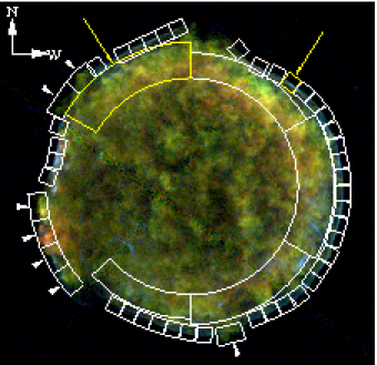
Figure 1.— Chandra three-color image of Tycho’s SNR after vignetting effects are corrected. Red, green, and blue represent 0.3–1.0 keV, 1.0–4.0 keV, and 4.0–8.0 keV X-rays, respectively. The image is binned by 0^′′.492 and has been smoothed by a Gaussian kernel of $\sigma=0^{\prime\prime}.984$. The intensity scale is square root. The small boxes, small annular pieces with triangular marks, and a large annulus divided by five sectors are where we investigate the proper motion of the forward shocks, ejecta knots, and reverse-shocked ejecta, respectively. We show an example one-dimensional X-ray profile from the yellow box indicated by an arrow in Fig. 3. Example $\chi^{2}$ or $C$ values calculated for the yellow box and the yellow annular sector with an arrow are shown in Fig. 4 and Fig. 6.

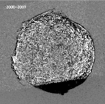
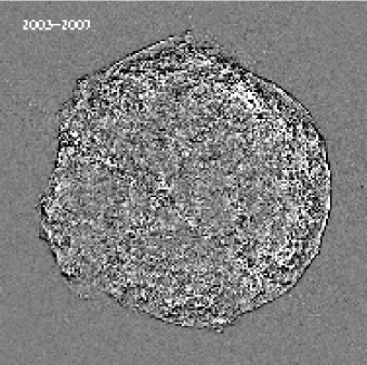
Figure 2.— Left: Difference image between 2000 and 2007 observations in 1.0–8.0 keV band. The original images before subtraction are binned by 0^′′.492 and smoothed using a Gaussian kernel of $\sigma=0^{\prime\prime}.492$. The intensity is linearly scaled from -3 to +3 counts pixel^-1. The southern dark (negative) region of the remnant is due to the fact that the observation in 2000 does not cover there. Right: Same as left but for 2003-2007. The structures running from NW to SE and from NE to SW are caused by the gaps of ACIS chips. Also visible artifacts are stripes running from NE to SW caused by bad columns.

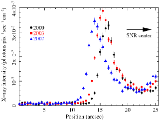
Figure 3.— Example one-dimensional profiles extracted from the yellow box shown in Fig. 1. Data points with black circles, red boxes, and blue triangles represent the 2000, 2003, and 2007 epochs, respectively.

Figure 4.— Example $\chi^{2}$- and $C$-value distributions as a function of shift position. The $\chi^{2}$ values with a solid line are calculated from the 2003 and 2007 one-dimensional profiles shown in Fig. 3 (see, section 3.1.1), while the $C$ values with a dashed line are calculated from 2003 and 2007 polar-coordinate images for the same region (see, section 3.1.2).

Figure 5.— Left: Proper motion for the forward shocks and the ejecta knots as a function of azimuthal angle (counterclockwise from the N). Black and red are derived from 2000-2007 and 2003-2007 measurements, respectively. Data points with filled boxes and open circles represent the forward shocks and the ejecta knots, respectively. The data for 2003-2007 measurements are displaced by 1 degree in azimuthal angle for clarity. The southern portion of the remnant (152^∘–229^∘ in azimuth angle) was not covered by the 2000 observation. Right: Same as left but for expansion rate (left axis) and expansion index (right axis).

Figure 6.— Example $C$-value distribution as a function of shift position for the reverse-shocked ejecta from the yellow (NE) annular sector in Fig. 1 calculated from 2003 and 2007 polar coordinated images.

Figure 7.— Same as Fig. 5 but for the reverse-shocked ejecta.

References

- (1) Albinson, J. S., Tuffs, R. J., Swinbank, E., & Gull, S. F. 1986, MNRAS, 219, 427
- (2) Baade, W. 1945, ApJ, 102, 309
- (3) Badenes, C., Borkowski, K. J., Hughes, J. P., Hwang, U., & Bravo, E. 2006, ApJ, 645, 1373
- (4) Badenes, C., Bravo, E., & Hughes, J. P. 2008, ApJ, 680, L33
- (5) Ballet, J. 2006, Adv. Space Res., 37, 1902
- (6) Bamba, A., Yamazaki, R., Yoshida, T., Terasawa, T., & Koyama, K. 2005, ApJ, 621, 793
- (7) Cash, W. 1979, ApJ, 228, 939
- (8) Cassam-Chenaï, G., Hughes, J. P., Ballet, J., and Decourchelle, A. 2007, ApJ, 665, 315
- (9) Decourchelle, A., Ellison, D. C., & Ballet, J. 2000, ApJ, 543, L57
- (10) Decourchelle, A., Sauvageot, J. L., Audard, M., Aschenbach, B.; Sembay, S., Rothenflug, R., Ballet, J., Stadlbauer, T., & West, R. G. 2001, A&A, 365, L218
- (11) DeLaney, T., & Rudnick, L. 2003, ApJ, 589, 818
- (12) Dwarkadas, V. V., & Chevalier, R. A. 1998, ApJ, 497, 807
- (13) Dwarkadas, V. V. 2000, ApJ, 541, 418
- (14) Ellison, D. C., Patnaude, D. J., Slane, P., Blasi, P., & Gabici, S. 2007, ApJ, 661, 879
- (15) Furuzawa, A., et al. 2009, ApJ, 693, L61
- (16) Hamuy, M., Phillips, M. M., Suntzeff, N. B., Schommer, R. A., Maza, J., & Aviles, R. 1996, AJ, 112, 239
- (17) Hernandez, J. I. G., Ruiz-Lapuente, P., Filippenko, A. V., Foley, R. J., Gal-Yam, A., & Simon, J. D. 2009, ApJ, 691, 1
- (18) Ihara, Y., Ozaki, J., Mamoru, D., Shigeyama, T., Kashikawa, N., Komiyama, Y., & Hattori, T. 2007, PASJ, 59, 811
- (19) Kamper, K. W., & van den Bergh, S. 1978, ApJ, 224, 851
- (20) Katsuda, S., Tsunemi, H., Mori, K. 2008, ApJ, 678, L35
- (21) Kerzendorf, W. E., Schmidt, B., P., Asplund, M., Nomoto, K., Podsiadlowski, P., Frebel, A., Fesen, R., A., & Yong, D. 2009, ApJ, 701, 1665
- (22) Kirshner, R. P., Winkler, P. F., & Chevalier, R. A. 1987, ApJ, 315, L135
- (23) Krause, O., Tanaka, M., Usuda, T., Hattori, T., Goto, M., Birkmann, S., & Nomoto, K. 2008, Nature, 456, 617
- (24) Lee, J.-J., Koo, B.-C., & Tatematsu, K. 2004, ApJ, 605L, 113
- (25) Hayato, A., et al. in preparation
- (26) Hughes, J. P. 2000, ApJ, 545, L53
- (27) Hwang, U., & Gotthelf E. V. 1997, ApJ, 475, 665
- (28) Hwang, U., Decourchelle, A., Holt, S. S., & Petre, R. 2002, ApJ, 581, 1101
- (29) Pohl, M., Yan, H., & Lazarian, A. 2005, ApJ, 626, L101
- (30) Pravdo, S. H., & Smith, B. W. 1979, ApJ, 234, L195
- (31) Reynolds, S. P., & Ellison, D. C. 1992, ApJ, 399, L75
- (32) Reynoso, E. M., Moffett, D. A., Goss, W. M., Dubner, G. M., Dickel, J. R.; Reynolds, S. P., & Giacani, E. B. 1997, ApJ, 491, 816
- (33) Reynoso, E. M., Velazquez, P. F., Dubner, G. M., & Goss, W. M. 1999, AJ, 117, 1827
- (34) Riess, A. G., et al. 1998, ApJ, 116, 1009
- (35) Ruiz-Lapuente, P. 2004, ApJ, 612, 357
- (36) Ruiz-Lapuente, P. et al. 2004, Nature, 431, 1069
- (37) Strom, R. G., Goss, W. M., & Shaver, P. A. 1982, MNRAS, 200, 473
- (38) Strom, R. G. 1983, in IAU Symp. 101, Supernova Remnants and thier X-ray Emission (Dordrecht: Reidel), 37
- (39) Tamagawa, T., et al. 2009, PASJ, 61, S167
- (40) Tan, S. M., & Gull, S. F. 1985, MNRAS, 216, 949
- (41) Uchiyama, Y., Aharonian, F. A., Tanaka, T., Takahashi, T., & Maeda, Y. 2007, Nature, 449, 576
- (42) Uchiyama, Y., & Aharonian, F. A. 2008, ApJL, 677, 105
- (43) Velazquez, P. F., Gomez, D. O., Dubner, G. M., de Castro, G. Gimenez, & Costa, A. 1998, A&A, 334, 1060
- (44) Vink, J. 2008, ApJ, 689, 231
- (45) Vlk, H. J., Berezhko, E. G., & Ksenofontov, L. T. 2008, A&A, 483, 529
- (46) Warren, J. et al. 2005, ApJ, 634, 376
- (47) Yang, X. J., Tsunemi, H., Lu, F. J., & Chen, L. 2009, ApJ, 692, 894