Kondo effect in a quantum dot coupled to ferromagnetic leads and side-coupled to a nonmagnetic reservoir

Abstract

Equilibrium transport properties of a single-level quantum dot tunnel-coupled to ferromagnetic leads and exchange-coupled to a side nonmagnetic reservoir are analyzed theoretically in the Kondo regime. The equilibrium spectral functions and conductance through the dot are calculated using the numerical renormalization group (NRG) method. It is shown that in the antiparallel magnetic configuration, the system undergoes a quantum phase transition with increasing exchange coupling $J$, where the conductance drops from its maximum value to zero. In the parallel configuration, on the other hand, the conductance is generally suppressed due to an effective spin splitting of the dot level caused by the presence of ferromagnetic leads, irrespective of the strength of exchange constant. However, for $J$ ranging from $J=0$ up to the corresponding critical value, the Kondo effect and quantum critical behavior can be restored by applying properly tuned compensating magnetic field.

I Introduction

Transport through a model single-level quantum dot captures many interesting and important features of transport phenomena in real quantum dots. One of such phenomena, which has been of great interest in the last decade, is the Kondo effect. goldhaber-gordon_98 ; cronenwett_98 ; hewson_book When the dot is occupied by a single electron, virtual transitions between the dot and electron reservoirs (external leads) cause spin fluctuations in the dot. As a result, the dot’s spin becomes screened by electrons of the reservoirs, which results in the formation of a non-local spin singlet ground state of the system. Furthermore, a resonance in the density of states appears at the Fermi level, which gives rise to enhanced transmission through the dot. In experiments, this leads to the well-known zero-bias anomaly, i.e. a peak at zero bias in the differential conductance. goldhaber-gordon_98 ; cronenwett_98

When the reservoirs are ferromagnetic, the effective exchange field generated by the electrodes may suppress the Kondo anomaly. LopezPRL03 ; martinekPRL03_2 ; martinekPRL03 ; ChoiPRL04 ; MatsubayashiPRB07 ; SimonPRB07 More specifically, when the dot described by an asymmetric Anderson model is symmetrically coupled to ferromagnetic leads, then the Kondo effect becomes suppressed in the parallel configuration, while in the antiparallel configuration the Kondo anomaly survives. However, the Kondo effect in the parallel configuration can be restored, when an external magnetic field, which compensates the exchange field created by the ferromagnetic leads, is applied. martinek_PRB05 ; sindel_PRB07 This behavior was confirmed in a couple of recent experiments. pasupathy_04 ; heersche_PRL06 ; hamayaAPL07 ; hamaya_PRB08 ; hauptmann_NatPhys08 ; parkinNL08

The situation becomes more complex and physically richer when the dot is exchange-coupled to an additional reservoir. OregPRL03 Such a model captures the essential physics of the so-called two-channel Kondo effect. Nozieres_JP80 ; Zawadowski_PRL80 ; AffleckPRB93 ; RalphPRL94 ; HettlerPRL94 ; AndreiPRL95 ; LebanonPRB03 ; FlorensPRL04 In the two-channel Kondo problem, two separate electron reservoirs (channels) compete with each other to screen the impurity’s spin. If the coupling to one of them is larger than to the other one, a usual single-channel Kondo state (spin singlet) is formed between the dot and more strongly coupled reservoir. This results in two competing Kondo ground states of the system, depending on the ratio of coupling strengths to the first and second conduction channels. Interestingly, these two Kondo states are separated by a quantum critical point, where both couplings are equal and an exotic two-channel Kondo state is formed, which cannot be described within the Landau Fermi-liquid theory. Very recently, the two-channel Kondo effect has been explored experimentally in quantum dots. PotokNature07 The experimental setup consisted of a small quantum dot coupled to external leads and to a large Coulomb-blockaded island. While the electrons could tunnel between the dot and the leads, only virtual tunneling processes between the dot and the island were allowed, resulting in an exchange coupling. By tuning the exchange coupling, it was possible to study the quantum phase transition between the two ground states of the system and analyze transport behavior in the non-Fermi liquid regime. PotokNature07 Theoretically, such a two-channel setup can be modelled for example by a quantum dot which is tunnel-coupled to external leads and exchange-coupled to another electron reservoir. PustilnikPRB04 ; tothPRB07 ; LiuJPCM08

As discussed above, both the Kondo effect in a quantum dot coupled to ferromagnetic leads and the two-channel Kondo phenomenon were already extensively studied. However, the interplay of leads’ ferromagnetism and two-channel Kondo effect remains to a large extent unexplored. Therefore, in this paper we address the two-channel Kondo problem in the presence of ferromagnetism. In particular, we consider an Anderson quantum dot coupled to ferromagnetic leads and exchange-coupled to a nonmagnetic electron reservoir. Using the numerical renormalization group (NRG) method, we analyze the interplay between the effects due to ferromagnetism of the leads and exchange coupling to the additional nonmagnetic reservoir. Depending on the strength of the tunnel coupling $t$ and exchange coupling $J$, the dot’s spin can be screened either by electrons in the ferromagnetic leads or by electrons in the nonmagnetic reservoir. By analyzing the equilibrium spectral functions and the conductance through the dot, we show that in the antiparallel magnetic configuration, the system undergoes a quantum phase transition with increasing exchange coupling $J$, where the conductance drops from the maximum value to zero. For a certain critical value of $J$, $J_{\rm c}^{\rm AP}$, both electron channels try to screen the dot’s spin and the conductance approaches a half of the quantum conductance. In the parallel configuration, on the other hand, the conductance is generally suppressed, irrespective of the exchange constant $J$, due to effective spin splitting of the dot level caused by the exchange field coming from ferromagnetic leads. martinekPRL03 ; ChoiPRL04 We show that the Kondo effect can be restored by applying a properly tuned external magnetic field $B$ for $J$ below the corresponding critical point, $J<\tilde{J}_{\rm c}^{\rm P}$. Furthermore, the quantum critical regime can also be recovered, which however requires a fine-tuning in the parameter space of $J$ and $B$.

The paper is organized as follows. In section II we present the model as well as briefly describe the NRG method together with some details of calculations. In turn, in section III we present numerical results for symmetric and asymmetric Anderson models in both parallel and antiparallel magnetic configurations of the system. Finally, we conclude in section IV.

II Theoretical description

II.1 Model

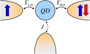
Figure 1: (color online) The schematic of a quantum dot (QD) tunnel-coupled to external ferromagnetic leads and exchange-coupled to a nonmagnetic electron reservoir. The spin-dependent coupling to the left (right) lead is described by $\Gamma_{\rm L\sigma}$ ($\Gamma_{\rm R\sigma}$), while $J$ denotes the exchange coupling constant. The magnetizations of the leads can form either parallel or antiparallel magnetic configuration, as indicated.

The considered system consists of a single-level quantum dot tunnel-coupled to left and right ferromagnetic leads and exchange-coupled to a nonmagnetic reservoir, see Fig. 1. It is assumed that the external leads are made of the same ferromagnetic material and their magnetizations are collinear, so that the system can be either in the parallel or antiparallel magnetic configuration. The total Hamiltonian is given by

$$H=H_{\rm FM}+H_{\rm NM}+H_{\rm QD}+H_{\rm tun}+H_{\rm exch}.$$ (1)

Here, $H_{\rm FM}$ describes the ferromagnetic leads, $H_{\rm FM}=\sum_{rk\sigma}\varepsilon_{rk\sigma}c^{\dagger}_{rk\sigma}c_{rk\sigma}$, where $c^{\dagger}_{rk\sigma}$ is the electron creation operator with wave number $k$, spin $\sigma$ in the left ($r={\rm L}$) or right ($r={\rm R}$) lead, and $\varepsilon_{rk\sigma}$ is the corresponding energy. The second part, $H_{\rm NM}$, corresponds to a nonmagnetic electron reservoir and is given by, $H_{\rm NM}=\sum_{k\sigma}\varepsilon_{k}a^{\dagger}_{k\sigma}a_{k\sigma}$, with $a^{\dagger}_{k\sigma}$ being the respective creation operator and $\varepsilon_{k}$ is the single-particle energy. The quantum dot is described by the Anderson Hamiltonian,

$$H_{\rm QD}=\sum_{\sigma}\varepsilon_{\rm d}d^{\dagger}_{\sigma}d_{\sigma}+Ud^{\dagger}_{\uparrow}d_{\uparrow}d^{\dagger}_{\downarrow}d_{\downarrow}+BS_{z},$$ (2)

where $d^{\dagger}_{\sigma}$ creates a spin-$\sigma$ electron, $\varepsilon_{\rm d}$ denotes the energy of an electron in the dot, and $U$ describes the Coulomb correlations between two electrons occupying the dot. The last term corresponds to external magnetic field $B$ applied along the $z$th direction ($g\mu_{B}\equiv 1$) and $S_{z}=\frac{1}{2}(d_{\uparrow}^{\dagger}d_{\uparrow}-d^{\dagger}_{\downarrow}d_{\downarrow})$. The tunnel Hamiltonian is given by

$$H_{\rm tun}=\sum_{rk\sigma}t_{r\sigma}\left(d_{\sigma}^{\dagger}c_{rk\sigma}+c_{rk\sigma}^{\dagger}d_{\sigma}\right),$$ (3)

where $t_{r\sigma}$ describes the spin-dependent hopping matrix elements between the dot and ferromagnetic leads. The coupling to magnetic leads can be described by $\Gamma_{r\sigma}=\pi\rho_{r}|t_{r\sigma}|^{2}$, where $\rho_{r}\equiv\rho$ is the density of states in the lead $r$. We have thus shifted the whole spin-dependence into the coupling constants and assumed a flat band of width $2D$, martinekPRL03 ; ChoiPRL04 where $D\equiv 1$ is set as the energy unit, if not stated otherwise.

By means of a unitary transformation in the left-right basis, Glazman98 ; Ng98 one can map the problem of tunneling through quantum dot coupled to the left and right leads into a problem where the dot is effectively coupled to a single lead with a new coupling constant, $\Gamma_{\sigma}=\Gamma_{\rm L\sigma}+\Gamma_{\rm R\sigma}$. This can be done by introducing the following symmetric operators, $\alpha_{k\sigma}=\tilde{t}_{\rm L\sigma}c_{{\rm L}k\sigma}+\tilde{t}_{\rm R\sigma}c_{{\rm R}k\sigma}$, with dimensionless coefficients $\tilde{t}_{r\sigma}=t_{r\sigma}/\sqrt{t^{2}_{\rm L\sigma}+t^{2}_{\rm R\sigma}}$. Then, the tunneling Hamiltonian can be written as

$$H_{\rm tun}=\sum_{k\sigma}\sqrt{\frac{\Gamma_{\sigma}}{\pi\rho}}\left(d_{\sigma}^{\dagger}\alpha_{k\sigma}+\alpha_{k\sigma}^{\dagger}d_{\sigma}\right).$$ (4)

One can see that now the dot is tunnel-coupled to only one effective electron reservoir, $H_{\rm FM}=\sum_{k\sigma}\varepsilon_{k\sigma}\alpha_{k\sigma}^{\dagger}\alpha_{k\sigma}$, with new spin-dependent coupling constant $\Gamma_{\sigma}$. The other parts of the system Hamiltonian, Eq. (1), are not affected by this transformation. To parameterize the spin-dependent couplings we also introduce the spin polarization of ferromagnetic leads, $p=(\Gamma_{\uparrow}-\Gamma_{\downarrow})/(\Gamma_{\uparrow}+\Gamma_{\downarrow})$. The couplings can be then written in a compact form as, $\Gamma_{\uparrow(\downarrow)}=(1\pm p)\Gamma$, where $\Gamma=(\Gamma_{\uparrow}+\Gamma_{\downarrow})/2$. Assuming symmetric coupling strength of the dot to the leads, the resultant coupling in the antiparallel configuration is the same for the spin-up and spin-down electrons, $\Gamma_{\uparrow(\downarrow)}^{\rm AP}=\Gamma$. On the other hand, in the parallel configuration, the couplings are then different for the two spin directions, $\Gamma_{\uparrow(\downarrow)}^{\rm P}=(1\pm p)\Gamma$, which effectively leads to spin splitting of the dot level and, when this is the case, the Kondo resonance may become suppressed because of broken spin degeneracy. martinekPRL03 ; ChoiPRL04

Finally, the exchange Hamiltonian describing the coupling between the dot and the second (nonmagnetic) reservoir is given by

$$H_{\rm exch}=\frac{J}{2}\sum_{\sigma\sigma^{\prime}}\sum_{k}\vec{S}a^{\dagger}_{k\sigma}\vec{\sigma}_{\sigma\sigma^{\prime}}a_{k\sigma^{\prime}},$$ (5)

where $\vec{S}=\frac{1}{2}\sum_{\sigma\sigma^{\prime}}d^{\dagger}_{\sigma}\vec{\sigma}_{\sigma\sigma^{\prime}}d_{\sigma^{\prime}}$ is the spin in the dot, $J$ denotes the exchange coupling constant and $\vec{\sigma}$ is a vector of Pauli spin matrices. We note that in addition to the exchange scattering of electrons [described by Eq. (5)] there could be also potential scattering. However, in this work we are mainly interested in the low energy physics, where the Kondo effect emerges, so the potential scattering may be neglected, as it does not lead to any Kondo-type correlations.

II.2 Method

To analyze the equilibrium transport properties of the considered system, we employ the numerical renormalization group method WilsonRMP75 – nonperturbative, very powerful and essentially exact numerical method to address quantum impurity problems. BullaRMP08 The NRG consists in a logarithmic discretization of the conduction band and mapping of the system onto a semi-infinite chain with the impurity (quantum dot) sitting at the end of the chain. By diagonalizing the Hamiltonian at consecutive sites of the chain and storing the eigenvalues and eigenvectors of the system, one can calculate the static and dynamic quantities of the system. In the case of model considered in this paper, the Hamiltonian is mapped onto two semi-infinite chains, where the first chain corresponds to ferromagnetic leads tunnel-coupled to the dot, while the second one to nonmagnetic reservoir exchange-coupled to the dot. Because such two-channel calculations are usually very demanding numerically, it is crucial to exploit as many symmetries of the system’s Hamiltonian as possible. Especially, using the $SU(2)$ symmetry decreases the size of Hilbert space and thus increases considerably the accuracy of calculations. In particular, to efficiently perform the analysis, we have used the flexible density-matrix numerical renormalization group (DM-NRG) code, which can tackle with arbitrary number of both Abelian and non-Abelian symmetries. Toth_PRB08 ; FlexibleDMNRG In calculations we have thus used the $U(1)$ symmetry for the $z$th component of the total spin, the $U(1)$ symmetry for the charge in the first channel, and the $SU(2)$ symmetry for the charge in the second channel. Furthermore, in calculations we have taken the discretization parameter $\Lambda=2$ and kept 3000 states at each iteration step.

Using the NRG we can calculate the spectral function of the dot, $A_{\sigma}(\omega)=-\frac{1}{\pi}{\rm Im}G^{R}_{d\sigma}(\omega)$, where $G_{d\sigma}^{R}(\omega)$ denotes the Fourier transform of the dot retarded Green’s function, $G_{d\sigma}^{R}(t)=-i\Theta(t)\langle\{d_{\sigma}(t),d_{\sigma}^{\dagger}(0)\}\rangle$. On the other hand, the spectral function can be directly related to the spin-resolved linear conductance $G_{\sigma}$ by the following formula

$$G_{\sigma}=\frac{e^{2}}{h}\frac{4\Gamma_{\rm L\sigma}\Gamma_{\rm R\sigma}}{\Gamma_{\rm L\sigma}+\Gamma_{\rm R\sigma}}\int d\omega\pi A_{\sigma}(\omega)\left(-\frac{\partial f(\omega)}{\partial\omega}\right),$$ (6)

where $f(\omega)$ is the Fermi distribution function and the total conductance is given by, $G=G_{\uparrow}+G_{\downarrow}$. At zero temperature, the spin dependent conductance for the parallel configuration is given by, $G_{\uparrow(\downarrow)}^{\rm P}=\frac{e^{2}}{h}(1\pm p)\pi\Gamma A_{\uparrow(\downarrow)}^{\rm P}$, while for the antiparallel configuration one gets, $G_{\uparrow(\downarrow)}^{\rm AP}=\frac{e^{2}}{h}(1-p^{2})\pi\Gamma A_{\uparrow(\downarrow)}^{\rm AP}=G^{\rm AP}/2$, where $A_{\sigma}^{\rm P/AP}$ is the zero-temperature spectral function of the $d$-level operator in respective magnetic configuration, taken at $\omega=0$.

III Numerical results

In the following we present numerical results on the equilibrium spectral function and linear conductance, when the quantum dot is in the Kondo regime. We will distinguish between two different situations; symmetric ($\varepsilon_{\rm d}=-U/2$) and asymmetric ($\varepsilon_{\rm d}\neq-U/2$) Anderson models. The origin of such a distinction stems from the way in which ferromagnetic leads act on the quantum dot. More specifically, in the asymmetric Anderson model ferromagnetism of the leads gives rise to a spin splitting of the Kondo resonance in the parallel configuration, while in the symmetric model no such a splitting appears (assuming that the dot is coupled with the same strength to the left and right leads). martinekPRL03 ; ChoiPRL04 ; martinek_PRB05 In other words, an effective exchange field, due to coupling to magnetic leads, acts on the dot in the former case, while such a field vanishes in the latter case. The effective field is directly related to the difference in the coupling strengths of the dot and ferromagnetic leads for the two spin orientations. Since the coupling in the spin-up channel is larger than that in the spin-down one, energy of the spin-up (spin-down) electron in the dot decreases (increases) by $\Delta\varepsilon_{\rm d}/2$. Consequently, the spin-dependent coupling acts as an effective magnetic field, leading to spin-splitting $\Delta\varepsilon_{\rm d}$ of the dot level. martinekPRL03 ; ChoiPRL04 ; martinek_PRB05

III.1 Symmetric Anderson model

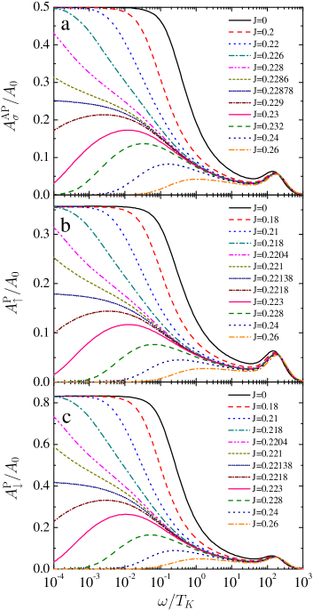
Figure 2: (color online) The spectral function of the $d$-level operator in the antiparallel (a) and parallel (b,c) magnetic configurations for the symmetric Anderson model and for different values of the exchange coupling $J$. The parameters are: $\varepsilon_{\rm d}=-0.05$, $U=0.1$, $\Gamma=0.0077$, $p=0.4$, and $T=0$. The Kondo temperature is defined as a half-width of the spectral function for $J=0$ and $p=0$, $T_{K}=2.5\times 10^{-4}$, while $A_{0}=\sum_{\sigma}A_{\sigma}(\omega=0)$ for $J=0$ and $p=0$. All the parameters are given in the units of $D\equiv 1$.

For the symmetric Anderson model we assume the following parameters (in the units of $D$), $\varepsilon_{\rm d}=-0.05$ and $U=0.1$. The zero-temperature spin-dependent spectral function $A_{\sigma}$, normalized to $A_{0}$, with $A_{0}=\sum_{\sigma}A_{\sigma}(\omega=0)$ taken for $J=0$ and $p=0$, is shown in Fig. 2 for both antiparallel (a) and parallel (b,c) magnetic configurations (note the logarithmic energy scale), and for indicated values of the exchange coupling parameter $J$. The spectral function is plotted as a function of $\omega/T_{K}$, where $T_{K}$ is the Kondo temperature defined as a half-width of the $d$-level spectral function for $J=0$ and $p=0$, $T_{K}=2.5\times 10^{-4}$. It can be seen that in the antiparallel configuration the spectral function is independent of the spin orientation [Fig. 2(a)], $A_{\uparrow}^{\rm AP}=A_{\downarrow}^{\rm AP}$, while it depends on electron spin in the parallel magnetic configuration, $A_{\uparrow}^{\rm P}\neq A_{\downarrow}^{\rm P}$, see Fig. 2(b) and (c). Note, that for symmetric Anderson model the spectral function is symmetric with respect to $\omega=0$, therefore here it is shown only for positive energies, i.e. for energies above the Fermi level. Moreover, note also that the spectral functions are normalized to that for the corresponding paramagnetic limit ($p=0$ and $J=0$), so $A_{\uparrow}(\omega=0)+A_{\downarrow}(\omega=0)\neq A_{0}$ in the parallel configuration.

Let us consider first the situation with vanishing exchange coupling of the dot to the nonmagnetic reservoir, $J=0$. For $\omega<T_{K}$, a Kondo peak develops in the dot spectral function due to screening of the dot’s spin by conduction electrons of ferromagnetic leads, which leads to the formation of a non-local spin singlet. The height of the Kondo peak is independent of spin in the antiparallel configuration and depends on spin in the parallel one. Apart from this, a Hubbard peak corresponding to $\varepsilon_{\rm d}+U$ is visible in the spectral function shown in Fig. 2. This behavior of the Kondo phenomenon in the presence of ferromagnetic leads is in agreement with that found by other methods, for instance by the equation of motion for the Green functions SwirkowiczPRB06 and also by the real-time diagrammatic technique. UtsumiPRB05

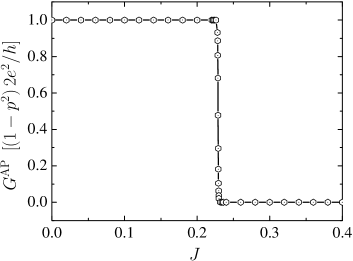
Figure 3: The linear conductance as a function of exchange coupling constant $J$ for the antiparallel magnetic configuration. The conductance was determined from the spectral function shown in Fig. 2(a). The parameters are the same as in Fig. 2 and $J$ is in units of $D=1$.

The situation changes when the electron in the dot is additionally exchange coupled to the nonmagnetic reservoir. When the coupling is antiferromagnetic and the coupling parameter $J$ increases, the width of the Kondo peak becomes gradually narrower and narrower. The hight of the peak, however, remains unchanged, as can be clearly seen in Fig. 2 for some small values of the exchange coupling constant. In order to see this behavior also for larger $J$, but still smaller than a critical value, $J=J_{\rm c}^{\rm P(AP)}$, one should plot the spectral function for lower energies. For $J<J_{\rm c}^{\rm P(AP)}$, the system is in the spin singlet ground state formed by the quantum dot spin and electrons in the ferromagnetic leads, which gives rise to the Kondo resonance in the spectral function. However, when $J>J_{\rm c}^{\rm P(AP)}$, the coupling to nonmagnetic reservoir becomes larger than the coupling to ferromagnetic leads and the dot’s spin becomes screened by electrons of the nonmagnetic reservoir. Now the Kondo peak in the spectral function disappears for both magnetic configurations of the system, see Fig. 2. When the two couplings are equal, i.e. for $J=J_{\rm c}^{\rm P(AP)}$, the system is in an exotic state where the two channels try to screen the dot’s spin. The spectral function at $\omega=0$ is then equal to a half of its value corresponding to $J=0$, $\frac{1}{2}A^{\rm P/AP}_{\sigma}|_{J=0}$, for both magnetic configurations, see Fig. 2. This behavior reveals a quantum phase transition with increasing strength of the exchange coupling. The origin of the phase transition follows from the interplay of the tunnel coupling to the ferromagnetic electrodes and exchange coupling to the nonmagnetic reservoir. More specifically, the quantum phase transition occurs at the boundary between two different singlet ground states, involving the dot’s spin and conduction electrons of the leads or side-coupled reservoir. The behavior of transport characteristics around this critical point in the case of nonmagnetic system was discussed in Ref. [PustilnikPRB04, ]. It was shown that the zero-temperature conductance depends step-like on the difference $\Delta$ between the tunnel and exchange couplings, and becomes equal to a half of its maximum value at the critical point, i.e. when $\Delta=0$. The discontinuity of the linear conductance with respect to $\Delta$ reflects the quantum phase transition in the parameter space of tunnel coupling $t$ and exchange coupling $J$. Since the conductance is determined by the corresponding spectral functions at $\omega=0$, quantum critical behavior is also reflected in the $J$-dependence of the spectral function. We also note that at finite temperature the transition is smeared as $\sqrt{T/T_{K}}$ and turns rather into a crossover. PustilnikPRB04

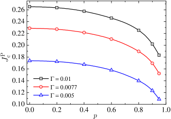
Figure 4: (color online) The dependence of the critical exchange coupling $J_{\rm c}^{\rm P}$ (in units of $D=1$) on the spin polarization of the leads $p$ in the case of symmetric Anderson model and parallel magnetic configuration for three different values of the tunnel coupling $\Gamma$, as indicated in the figure. The other parameters are the same as in Fig. 2.

Using the Schrieffer-Wolff transformation, Schrieffer-Wolff one could try to estimate the critical value of $J$. For the symmetric Anderson model and for antiparallel configuration one gets, hewson_book $J^{\rm S-W}_{\rm c}=\Gamma(\pi\rho)^{-1}U|\varepsilon_{\rm d}|^{-1}(\varepsilon_{\rm d}+U)^{-1}\approx 0.196$. From the numerical data, however, one finds $J_{\rm c}^{\rm AP}\approx 0.22878$ for the antiparallel and $J_{\rm c}^{\rm P}\approx 0.22138$ for the parallel configurations, see Fig. 2. The difference between the value obtained using the Schrieffer-Wolff transformation and the numerical value may result for example from the fact that the transformation is based on perturbation expansion, and takes into account only the second-order tunneling processes.

The quantum critical behavior can be also seen in the dependence of the linear conductance on the coupling constant $J$, which is shown in Fig. 3 for the antiparallel magnetic configuration. For $J<J_{\rm c}^{\rm AP}$, the conductance is $G^{\rm AP}=(1-p^{2})2e^{2}/h$ and drops to zero when $J>J_{\rm c}^{\rm AP}$. On the other hand, at the quantum critical point $J=J_{\rm c}^{\rm AP}$, the linear conductance is equal to half of its value for $J=0$, i.e. $G^{\rm AP}=(1-p^{2})e^{2}/h$. Consequently, the dependence of the conductance on the exchange coupling $J$ can be expressed as $G^{\rm AP}=\Theta(\Delta)(1-p^{2})2e^{2}/h$, where $\Delta=J_{\rm c}^{\rm AP}-J$ and $\Theta(x)$ is the step function. The dependence of $G$ on $J$ for the parallel configuration is qualitatively similar to that in the antiparallel configuration, therefore it is not shown here.

In Fig. 4 the dependence of the critical exchange coupling $J_{\rm c}^{\rm P}$ on the spin polarization of the leads $p$ in the case of symmetric Anderson model and parallel magnetic configuration is shown for three different values of the tunnel coupling $\Gamma$. First of all, the critical coupling $J_{\rm c}^{\rm P}$ decreases with decreasing the coupling strength $\Gamma$. Moreover, $J_{\rm c}^{\rm P}$ also decreases with increasing the spin polarization of the leads. For $p\to 1$, $J_{\rm c}^{\rm P}$ tends to zero, as only spins of one orientation are coupled to the leads and the Kondo effect becomes suppressed. This behavior of the critical parameter $J_{\rm c}^{\rm P}$ is consistent with the dependence of the Kondo temperature in a quantum dot coupled to ferromagnetic leads on the coupling strength $\Gamma$ and spin polarization $p$. LopezPRL03 ; martinekPRL03_2 ; martinekPRL03 ; ChoiPRL04 ; sindel_PRB07

III.2 Asymmetric Anderson model

Let us now consider the case of asymmetric Anderson model, $|\varepsilon_{\rm d}|\neq U/2$. For numerical calculations we assume $\varepsilon_{\rm d}=-0.05$ and $U=0.2$. The spectral function in the antiparallel magnetic configuration as a function of $\omega/T_{K}$, where $T_{K}=3.4\times 10^{-5}$, is shown in Fig. 5 for indicated values of the exchange coupling parameter $J$. The inset shows the behavior of the spectral function associated with the Kondo peak. The general features of the spectral function are similar to those of the corresponding spectral function in the case of symmetric Anderson model discussed above, see Fig. 2. This is because in the antiparallel configuration the resultant coupling to ferromagnetic leads does not depend on spin and the system effectively behaves as a nonmagnetic one. As before, one observes a quantum phase transition at $J=J_{\rm c}^{\rm AP}$, where now $J_{\rm c}^{\rm AP}\approx 0.1858$. The only difference is that for $|\varepsilon_{\rm d}|\neq U/2$ the spectral function displays an asymmetric behavior with respect to $\omega=0$, see the inset in Fig. 5.

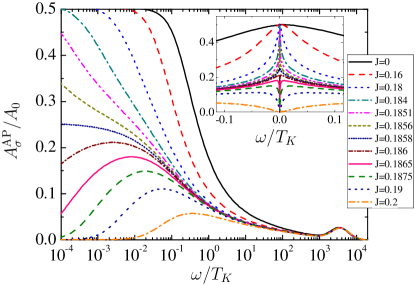
Figure 5: (color online) The spectral function of the $d$-level operator in the antiparallel magnetic configuration for the asymmetric Anderson model, $\varepsilon_{\rm d}=-0.05$, $U=0.2$, and for indicated values of the exchange coupling $J$. The Kondo temperature for assumed parameters (and for $J=0$ and $p=0$) is $T_{K}=3.4\times 10^{-5}$. The other parameters are the same as in Fig. 2.

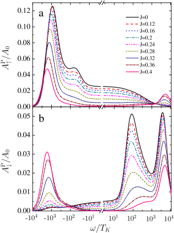
Figure 6: (color online) The spectral function of the $d$-level operator in the parallel magnetic configuration for the asymmetric Anderson model. The other parameters are the same as in Fig. 5.

The situation, however, changes significantly when the magnetizations of the leads switch to the parallel configuration. The corresponding spectral function for spin-$\uparrow$ and spin-$\downarrow$ is shown in Fig. 6. Note, that now the spectral function is shown for both positive and negative energies. As before, let us consider first the case of $J=0$. Due to an effective exchange field originating from the presence of ferromagnetic electrodes, the spin degeneracy of the dot level is lifted. At zero temperature, the magnitude of the splitting due to exchange field, $\Delta\varepsilon_{\rm d}$, can be estimated from the formula martinekPRL03 ; ChoiPRL04 ; martinek_PRB05

$$\Delta\varepsilon_{\rm d}=\frac{2p\Gamma}{\pi}\frac{|\varepsilon_{\rm d}|}{|\varepsilon_{\rm d}+U|}\,.$$ (7)

For the assumed parameters one then finds, $\Delta\varepsilon_{\rm d}\approx 2.15\times 10^{-3}$. The exchange field leads generally to the suppression of the Kondo peak, however the reminiscent of the Kondo effect are still visible as relatively small peaks in the $d$-level spectral function. The position of these peaks is shifted away from the Fermi level – to positive energies for spin-$\downarrow$ and to negative energies for spin-$\uparrow$. In fact, the peaks occur for energies comparable to the magnitude of the exchange field. As can be seen in Fig. 6, they develop at $\omega/T_{K}\approx 10^{2}$ for spin-$\downarrow$ and at $\omega/T_{K}\approx-10^{2}$ for spin-$\uparrow$ components of the spectral function. The other peaks in the spectral functions correspond to the dot level $\varepsilon_{\rm d}$ and its Coulomb counterpart $\varepsilon_{\rm d}+U$.

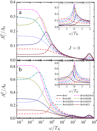
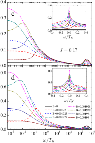
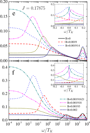
Figure 7: (color online) The spectral function of the $d$-level operator in the parallel magnetic configuration for the asymmetric Anderson model in the presence of external magnetic field $B$ applied along the $z$th direction for different values of exchange coupling constant $J=0$ (a,b), $J=0.17$ (c,d) and $J=0.17875$ (e,f). The other parameters are the same as in Fig. 5.

When the coupling parameter $J$ increases, the weak Kondo resonances in the spectral function gradually disappear for both spin orientations. The physics behind this disappearance remains similar to that described above, i.e. screening of the dot’s spin by the nonmagnetic reservoir exchange-coupled to the dot. Interestingly, there is no quantum phase transition in the case of parallel magnetic configuration shown in Fig. 6.

Let us now assume that there is an external magnetic field $B$ applied to the dot along the $z$th direction. In the case of antiparallel configuration, the magnetic field destroys both the Kondo resonance and quantum phase transition with changing $J$. However, when the leads are aligned in parallel, the Kondo effect is already suppressed by the effective exchange field coming from ferromagnetic electrodes, and one may consider the possibility of restoring the Kondo peak by applying an external magnetic field which compensates the effects due to exchange field. In Fig. 7 we show the spectral functions for the parallel magnetic configuration in the case of an asymmetric Anderson model, calculated for three different values of the exchange constant $J$ in the presence of external magnetic field $B$. The insets display behavior of the spectral function associated with the Kondo peaks. When $J=0$, see Fig. 7(a) and (b), the full Kondo peak at the Fermi level in the spectral density can be restored for both spin orientations by properly tuned external magnetic field, which happens for $B=B_{\rm c}=0.0020545$, where $B_{\rm c}$ (in the units of D) denotes the compensating field. This is in agreement with the result obtained earlier. martinekPRL03 ; ChoiPRL04 Similar behavior also appears for larger positive $J$, e.g. for $J=0.17$ shown in Fig. 7(c) and (d). Now, the Kondo resonance becomes restored when the compensating field is $B_{\rm c}=0.001928$. Note that the magnitude of magnetic field necessary for full restoration of the Kondo effect slightly decreases as $J$ increases. The question which arises now is whether such a restoration by magnetic field is also possible for larger values of $J$. By fine-tuning in the parameter space of $J$ and $B$, we have found that this is the case for $J$ below a certain critical value $J<\tilde{J}_{\rm c}^{\rm P}=0.17875$. Here $\tilde{J}_{\rm c}^{\rm P}$ denotes the critical value of $J$ in the parallel configuration and in the presence of the compensating magnetic field. From numerical results (not shown here), follows that for $J>\tilde{J}_{\rm c}^{\rm P}$, the magnetic field can only partially restore the Kondo effect, leading to small side peaks in the spectral function, while the full Kondo peak at $\omega=0$ cannot be restored. One may now expect that for $J=\tilde{J}_{\rm c}^{\rm P}$, the magnetic field should also restore the quantum critical state. Indeed, by fine-tuning in the parameter space we have found that the quantum critical state can be recovered for $B_{\rm c}=0.00191621$. This situation is shown explicitly in Fig. 7(e) and (f). Thus, we have shown that in the parallel configuration the properly-tuned magnetic field can restore both the full Kondo effect for $J<\tilde{J}_{\rm c}^{\rm P}$ as well as the quantum critical state for $J=\tilde{J}_{\rm c}^{\rm P}$.

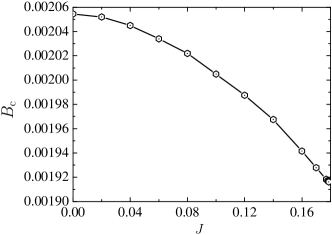
Figure 8: The dependence of the compensating magnetic field $B_{\rm c}$ on the exchange coupling constant $J$ in the case of the parallel configuration and asymmetric Anderson model. The other parameters are the same as in Fig. 5. $J$ and $B_{\rm c}$ are in units of $D=1$.

By comparing numerical curves presented in Fig. 7, one can note that the compensating field $B_{\rm c}$ decreases with increasing the exchange coupling $J$. This is explicitly shown in Fig. 8, where we have calculated the dependence of $B_{\rm c}$ on the exchange coupling $J$. For $J<\tilde{J}_{\rm c}^{\rm P}$, the Kondo resonance can be fully restored by applying compensating field $B_{\rm c}$. On the other hand, when $J>\tilde{J}_{\rm c}^{\rm P}$, the magnetic field cannot compensate the exchange field, so the notion of compensating field becomes meaningless.

IV Conclusions

In this paper we have considered spectral and transport properties of a single-level quantum dot connected to external ferromagnetic leads and exchange-coupled to a nonmagnetic reservoir. Using the numerical renormalization group method we have calculated the zero-temperature $d$-level spectral function and the conductance through the dot. We have shown that in the antiparallel configuration, depending on the strength of the exchange interaction $J$, the Kondo singlet ground state can form, in which the conduction electrons either in the ferromagnetic leads or in the nonmagnetic reservoir are involved. In the former case, the conductance is maximum, whereas in the latter case the conductance becomes fully suppressed. For a certain critical value of $J$, $J_{\rm c}^{\rm AP}$, both electron channels try to screen the dot’s spin and the conductance is equal to a half of its maximum value. The boundary between the two ground states is a quantum phase transition.

In the parallel magnetic configuration, on the other hand, the Kondo effect is generally destroyed due to an effective spin splitting of the dot level caused by the presence of ferromagnetic leads. However, there are still small side peaks – reminiscent of the Kondo effect – which occur on both sides of the Fermi level for energies of the order of effective exchange field. Nevertheless, with increasing the exchange constant $J$, these peaks become suppressed.

We have also considered the influence of an external magnetic field on the $d$-level spectral function and shown that in the parallel configuration the Kondo effect can be restored by applying appropriately tuned compensating magnetic field for $J<\tilde{J}_{\rm c}^{\rm P}$, where $\tilde{J}_{\rm c}^{\rm P}$ is the critical value of $J$ in the compensating magnetic field. If, however, $J>\tilde{J}_{\rm c}^{\rm P}$, the full Kondo effect cannot be restored by a magnetic field. In addition, we have found that the quantum critical behavior, which is suppressed in the parallel configuration, can also be recovered by tuning the external magnetic field.

- (1) D. Goldhaber-Gordon, H. Shtrikman, D. Mahalu, D. Abusch-Magder, U. Meirav, and M. A. Kastner, Nature (London) 391, 156 (1998).
- (2) S. Cronenwett, T. H. Oosterkamp, and L. P. Kouwenhoven, Science 281, 182 (1998).
- (3) A. C. Hewson, The Kondo Problem to Heavy Fermions (Cambridge University Press, Cambridge, 1993).
- (4) Rosa Lopez and David Sanchez, Phys. Rev. Lett. 90, 116602 (2003).
- (5) J. Martinek, Y. Utsumi, H. Imamura, J. Barnaś, S. Maekawa, J. König, and G. Schön, Phys. Rev. Lett. 91, 127203 (2003).
- (6) J. Martinek, M. Sindel, L. Borda, J. Barnaś, J. König, G. Schön, and J. von Delft, Phys. Rev. Lett. 91, 247202 (2003).
- (7) Mahn-Soo Choi, David Sanchez, and Rosa Lopez, Phys. Rev. Lett. 92, 056601 (2004).
- (8) Daisuke Matsubayashi and Mikio Eto, Phys. Rev. B 75, 165319 (2007).
- (9) P. Simon, P. S. Cornaglia, D. Feinberg, and C. A. Balseiro, Phys. Rev. B 75, 045310 (2007).
- (10) J. Martinek, M. Sindel, L. Borda, J. Barnaś, R. Bulla, J. König, G. Schön, S. Maekawa, J. von Delft, Phys. Rev. B 72, 121302(R) (2005).
- (11) M. Sindel, L. Borda, J. Martinek, R. Bulla, J. König, G. Schön, S. Maekawa, and J. von Delft, Phys. Rev. B 76, 045321 (2007).
- (12) A. N. Pasupathy, R. C. Bialczak, J. Martinek, J. E. Grose, L. A. K. Donev, P. L. McEuen, and D. C. Ralph, Science 306, 86 (2004).
- (13) H. B. Heersche, Z. de Groot, J. A. Folk, L. P. Kouwenhoven, H. S. van der Zant, A. A. Houck, J. Labaziewicz, and I. L. Chuang, Phys. Rev. Lett. 96, 017205 (2006).
- (14) K. Hamaya, M. Kitabatake, K. Shibata, M. Jung, M. Kawamura, K. Hirakawa, T. Machida, T. Taniyama, S. Ishida and Y. Arakawa, Appl. Phys. Lett. 91, 232105 (2007).
- (15) K. Hamaya, M. Kitabatake, K. Shibata, M. Jung, M. Kawamura, S. Ishida, T. Taniyama, K. Hirakawa, Y. Arakawa, and T. Machida, Phys. Rev. B 77, 081302(R) (2008).
- (16) J. Hauptmann, J. Paaske, P. Lindelof, Nature Phys. 4, 373 (2008).
- (17) H. Yang, S.-H. Yang, S. S. P. Parkin, Nano Lett. 8, 340 (2008).
- (18) Y. Oreg and D. Goldhaber-Gordon, Phys. Rev. Lett. 90, 136602 (2003).
- (19) P. Nozieres and A. Blandin, J. Phys. 41, 193 (1980).
- (20) A. Zawadowski, Pys. Rev. Lett. 45, 211 (1980).
- (21) I. Affleck, A. W. W. Ludwig, Phys. Rev. B 48, 7297 (1993).
- (22) D. C. Ralph, A. W. W. Ludwig, J. von Delft, R. A. Buhrman, Phys. Rev. Lett. 72, 1064 (1994).
- (23) M. H. Hettler, J. Kroha, S. Hershfield, Phys. Rev. Lett. 73, 1967 (1994).
- (24) N. Andrei and A. Jerez, Phys. Rev. Lett. 74, 4507 (1995).
- (25) E. Lebanon, A. Schiller, F. B. Anders, Phys. Rev. B 68, 155301 (2003).
- (26) S. Florens, A. Rosch, Phys. Rev. Lett. 92, 216601 (2004).
- (27) R. M. Potok, I. G. Rau, Hadas Shtrikman, Yuval Oreg, and D. Goldhaber-Gordon, Nature 446, 167 (2007).
- (28) M. Pustilnik, L. Borda, L. I. Glazman, and J. von Delft, Phys. Rev. B 69, 115316 (2004).
- (29) A. I. Tóth, L. Borda, J. von Delft, and G. Zárand, Phys. Rev. B 76, 155318 (2007).
- (30) Y. S. Liu X. F. Yang, X. H. Fan and Y. J. Xia, J. Phys.: Condens. Matter 20, 135226 (2008).
- (31) L. I. Glazman and M. E. Raikh, JETP Lett. 47, 452 (1988).
- (32) T. K. Ng and P. A. Lee, Phys. Rev. Lett. 61, 1768 (1988).
- (33) K. G. Wilson, Rev. Mod. Phys. 47, 773 (1975).
- (34) R. Bulla, T. A. Costi, and T. Pruschke Rev. Mod. Phys. 80, 395 (2008).
- (35) A. I. Tóth, C. P. Moca, O. Legeza, and G. Zaránd, Phys. Rev. B 78, 245109 (2008).
- (36) O. Legeza, C. P. Moca, A. I. Tóth, I. Weymann, G. Zaránd, arXiv:0809.3143 (2008) (unpublished).
- (37) R. Świrkowicz, M. Wilczyński, M. Wawrzyniak, and J. Barnaś, Phys. Rev. B 73, 193312 (2006).
- (38) Y. Utsumi, J. Martinek, G. Schön, H. Imamura, and S. Maekawa, Phys. Rev. B 71, 245116 (2005).
- (39) J. R. Schrieffer and P. A. Wolff, Phys. Rev. 149, 491 (1966).