Link Prediction Based on Local Random Walk

Abstract

The problem of missing link prediction in complex networks has attracted much attention recently. Two difficulties in link prediction are the sparsity and huge size of the target networks. Therefore, the design of an efficient and effective method is of both theoretical interests and practical significance. In this Letter, we proposed a method based on local random walk, which can give competitively good prediction or even better prediction than other random-walk-based methods while has a lower computational complexity.

1 Introduction

Recently, the problem of missing link prediction in complex network has attracted much attention [1, 2, 3]. Link prediction aims at estimating the likelihood of the existence of a link between two nodes. For some networks, especially biological networks such as protein-protein interaction networks, metabolic networks and food webs, the discovery of links (i.e., interactions) is costly in the laboratory or the field, and thus the current knowledge of those networks is substantially incomplete [4, 5]. Instead of blindly checking all the possible interactions, predicting based on the observed interactions and focusing on those links most likely to exist can sharply reduce the experimental costs if the predictions are accurate enough [1]. For some others like web-based friendship networks, very likely but not yet existent links can be suggested to users as recommendations of promising friendships, which can help users in finding new friends and thus enhance their loyalties to the web sites. In addition, the link prediction algorithms can be applied to solve the classification problem in partially labeled networks [6], such as to distinguish the research areas of scientific publications.

Commonly, two nodes are more likely to be connected if they are more similar, where a latent assumption is that the link itself indicates a similarity between the two endpoints and this similarity can be transferred through the links. In this case, the similarity indices are used to quantify the structural equivalence (see, for example the Leicht-Holme-Newman index [7] and the transferring similarity [8]). However, in some networks the two endpoints of one link are not essentially similar, such as the sexual network [9] and the word networks. In these cases, we can use the regular equivalence (see Ref. [10], for mathematical definition of regular equivalence), which indicates that two nodes are said to be similar if they have connected to the similar nodes. How to predict missing links in such kind of networks is still an open problem to us. Our study focuses on structure equivalence.

Node similarity can be defined by the essential attributes of nodes. For example, if two persons have same age, sex and job, we can say that they are similar. Another group of similarity is based only on the network structure. An introduction and comparison of some similarity indices is presented in Ref. [2], where the Common Neighbours [11], Jaccard coefficient [12], Adamic-Adar Index [13] and Preferential Attachment [14] are the node-dependent indices that require only the information about node degree and the nearest neighborhood, while the Katz Index [15], Hitting Time [16], Commute Time [17], Rooted PageRank [18], SimRank [19] and Blondel Index [20] belong to the path-dependent indices that ask for global knowledge of the network topology. In Ref. [21], Zhou et al. proposed two new local indices, Resource Allocation index and Local Path index. Empirical results show that these two indices perform very well among all known local indices. In particular, the local path index, asking for a little bit more information than common neighbours, provides competitively accurate prediction compared with the global index [22]. Lü and Zhou [23] studied the link prediction problem in weighted networks, and found that the weak links may play a more important role than strong links. Besides, Clauset et al. [1] proposed an algorithm based on the hierarchical network structure, which gives good predictions for the networks with hierarchical structures, such as grassland species food web and terrorist association network. In real application, similarity indices only exploiting local information are more efficient than those based on global information, for their lower computational complexity. However, due to the insufficient information, local indices may be less effective for their low prediction accuracy. To design an efficient and effective algorithm is a main challenge in link prediction.

In this Letter, we define the node similarity based on local random walk, which has lower computational complexity compared with other random-walk-based similarity indices, such as average commute time (ACT) and random walk with restart (RWR). We compare our method with five representative similarity indices, including three local ones (common neighbours, resource allocation and local path indices) and two global ones (ACT and RWR), as well as the hierarchical structure method. Empirical results on five real networks show that our method performs best.

Table 1: The basic topological features of the giant components of the five example networks. $N$ and $|E|$ are the total numbers of nodes and links, respectively. $\langle{k}\rangle$ is the average degree of the network. $\langle{d\rangle}$ is the average shortest distance between node pairs. $C$ and $r$ are clustering coefficient [34] and assortative coefficient [36], respectively. $H$ is the degree heterogeneity, defined as $H=\frac{\langle k^{2}\rangle}{\langle k\rangle^{2}}$.

Networks	$N$	$|E|$	$\langle k\rangle$	$\langle d\rangle$	$C$	$r$	$H$
USAir	332	2126	12.807	2.46	0.749	-0.208	3.464
NetScience	379	941	4.823	4.93	0.798	-0.082	1.663
Power	4941	6594	2.669	15.87	0.107	0.003	1.450
Yeast	2375	11693	9.847	4.59	0.388	0.454	3.476
C.elegans	297	2148	14.456	2.46	0.308	-0.163	1.801

2 Similarity Based on Local Random Walk

Consider an undirected simple network $G(V,E)$, where $V$ is the set of nodes and $E$ is the set of links. Multiple links and self-connections are not allowed. For each pair of nodes, $x,y\in V$, we assign a score, $s_{xy}$. In this Letter, we adopt the simplest framework, that is, to directly set the similarity as the score. All the nonexistent links are sorted in descending order according to their scores, and the links at the top are most likely to exist.

Random walk is a Markov chain describing the sequence of nodes visited by a random walker [24, 25]. This process can be described by the transition probability matrix, $P$, with $P_{xy}=a_{xy}/k_{x}$ presenting the probability that a random walker staying at node $x$ will walk to $y$ in the next step, where $a_{xy}$ equals 1 if node $x$ and node $y$ are connected, 0 otherwise, and $k_{x}$ denotes the degree of node $x$. Given a random walker starting from node $x$, denoting by $\pi_{xy}(t)$ the probability that this walker locates at node $y$ after $t$ steps, we have

$$\vec{\pi_{x}}(t)=P^{T}\vec{\pi_{x}}(t-1),$$ (1)

where $\vec{\pi_{x}}(0)$ is an $N\times{1}$ vector with the $x^{th}$ element equal to 1 and others all equal to 0, and $T$ is the matrix transpose. The initial resource is usually assigned according to the importance of nodes [26]. Here, we simply set the initial resource of node $x$ proportional to its degree $k_{x}$. Then, after normalization the similarity between node $x$ and node $y$ is

$$s^{LRW}_{xy}(t)=\frac{k_{x}}{2|E|}\cdot\pi_{xy}(t)+\frac{k_{y}}{2|E|}\cdot\pi_{yx}(t),$$ (2)

where $|E|$ is the number of links in the network. It is obvious that $s_{xy}=s_{yx}$. Note that, here we only focus on the few-step random walk not the stationary state which can be characterized by the eigenvector centrality [27, 28]. In the stationary state, we have $\pi_{xy}=\frac{k_{x}}{2|E|}$, and thus according to Eq. 2, $s_{xy}=\frac{k_{x}\cdot{k_{y}}}{2|E|^{2}}$, which is equivalent to the preferential attachment index (i.e., $k_{x}\cdot{k_{y}}$) that has been discussed in Ref. [21].

One difficulty with all random-walk-based similarity measures is their sensitive dependence to parts of the network far away from target nodes [2]. For example, in a random walk from $x$ to $y$, the walker has a certain probability to go too far away from both $x$ and $y$ although they may be close to each other. This may lead to a low prediction accuracy since in most real networks nodes tend to connect with the ones nearby rather than far away. This feature relates to the high clustering or locality of networks. A possible way to counteract this dependence is to continuously release the walkers at the starting point, resulting in a higher similarity between the target node and the nodes nearby. By superposing the contribution of each walker (walkers move independently), we obtain the similarity index:

$$s_{xy}^{SRW}(t)=\sum_{l=1}^{t}s_{xy}^{LRW}(l),$$ (3)

where SRW is the abbreviation for superposed random walk.

3 Metrics

To test the algorithm’s accuracy, the observed links, $E$, are randomly divided into two parts: the training set, $E^{T}$, and the probe set, $E^{P}$. Clearly, $E=E^{T}\cup E^{P}$ and $E^{T}\cap E^{P}={\o}$. We use two standard metrics, AUC [29] and precision [32], to quantify the accuracy of prediction algorithms. The former evaluates the overall ranking resulted from the algorithm, while the later focuses on the top-L candidates. In the present case, AUC can be interpreted as the probability that a randomly chosen missing link (a link in $E^{P}$) is given a higher score than a randomly chosen nonexistent link (a link in $U\setminus E$, where $U$ denotes the universal set). In the implementation, among $n$ independent comparisons, if there are $n^{\prime}$ times the missing link having a higher score and $n^{\prime\prime}$ times they are of the same score, we have

$$AUC=\frac{n^{\prime}+0.5n^{\prime\prime}}{n}.$$ (4)

If all the scores are generated from an independent and identical distribution, the AUC should be about 0.5. Therefore, the degree to which the AUC exceeds 0.5 indicates how much better the algorithm performs than pure chance. Precision is defined as the ratio of relevant items to the number of selected items. In our case, to calculate precision we firstly need to rank all the nonexistent links in decreasing order according to their score. Then we focus on the top-$L$ (here $L=100$) links. If there are $l$ links successfully predicted (i.e., in the probe set), then

$$Precision=\frac{l}{L}.$$ (5)

Clearly, higher value of precision means higher prediction accuracy.

4 Data

We consider five representative networks drawn from disparate fields: (i) USAir: The network of the US air transportation system, which contains 332 airports and 2126 airlines. (ii) NetScience: A network of coauthorships between scientists who are themselves publishing on the topic of network science [33]. This network contains 1589 scientists, 128 of which are isolated. In fact, it consists 268 components, and the size of the giant component is only 379. (iii) Power Grid: An electrical power grid of the western US [34], with nodes representing generators, transformers and substations, and edges corresponding to the high voltage transmission lines between them. (iv) Yeast: A protein-protein interaction network of yeast containing 2617 proteins and 11855 interactions [35]. Although this network is not well connected (it contains 92 components), most of the nodes belong to the giant component, whose size is 2375. (v) C.elegans: The neural network of the nematode worm C.elegans, in which an edge joins two neurons if they are connected by either a synapse or a gap junction [34]. In this Letter, we only consider the giant component, because the similarity indices based on local random walk, as well as those well-known indices (except the preferential attachment index) reported in Refs. [2, 21], will give zero score to a pair of nodes located in two disconnected components. This implies that if a network is unconnected, we actually predict the links in each component separately, and any probe link connecting two components can not be predicted. Therefore we need to make sure that the training set represents a connected network. Actually, each time before moving a link to the probe set, we first check if this removal will make the training network disconnected. Table 1 summarizes the basic topological features of the giant components of those networks.

Table 2: Comparison of algorithms’ accuracy quantified by AUC and Precision. For each network, the training set contains 90% of the known links. Each number is obtained by averaging over 1000 implementations with independently random divisions of training set and probe set. We set the parameters $\varepsilon=10^{-3}$ in LP and $c=0.9$ in RWR. The numbers inside the brackets denote the optimal step of LRW and SRW indices. For example, 0.9723(2) means the optimal AUC is obtained at the second step of LRW. The highest accuracy in each line is emphasized by black. For HSM we generate 5000 samples of dendrograms for each implementation.

AUC	CN	RA	LP	ACT	RWR	HSM	LRW	SRW
USAir	0.9542	0.9723	0.9524	0.9012	0.9765	0.9038	0.9723(2)	0.9782(3)
NetScience	0.9784	0.9825	0.9855	0.9338	0.9928	0.9295	0.9893(4)	0.9917(3)
Power	0.6257	0.6258	0.6974	0.8948	0.7599	0.5025	0.9532(16)	0.9631(16)
Yeast	0.9151	0.9163	0.9700	0.8997	0.9782	0.6720	0.9744(7)	0.9801(8)
C.elegans	0.8492	0.8705	0.8672	0.7470	0.8888	0.8082	0.8986(3)	0.9062(3)
Precision	CN	RA	LP	ACT	RWR	HSM	LRW	SRW
USAir	0.5907	0.6350	0.6078	0.4887	0.6519	0.2764	0.6435(3)	0.6724(3)
NetScience	0.2618	0.5442	0.3007	0.1911	0.5485	0.2502	0.5442(2)	0.5442(2)
Power	0.1121	0.0806	0.1284	0.0813	0.0863	0.0040	0.0806(2)	0.1140(3)
Yeast	0.6707	0.4949	0.6823	0.5680	0.5217	0.8408	0.8591(3)	0.7268(9)
C.elegans	0.1222	0.1266	0.1391	0.0654	0.1305	0.0763	0.1399(3)	0.1407(3)

Figure 1: (Color online) Dependence of AUC and Precision on the size of training set in USAir and C.elegans. Each number is obtained by averaging over 1000 implementations with independently random divisions of the training set and probe set. For HSM we generate 5000 samples of dendrograms for each implementation.

5 Results and Discussion

We compare the LRW index and SRW index with other five similarity indices, including three local ones: Common Neighbour (CN), Resource Allocation index (RA) and Local Path index (LP), and two global ones: Average Commute Time (ACT), Random Walk with Restart (RWR), as well as the Hierarchical Structure method (HSM). A brief introduction of each algorithm is shown as follow:

(i) CN: For a node $x$, let $\Gamma(x)$ denote the set of neighbours of $x$. By common sense, two nodes, $x$ and $y$, are more likely to have a link if they have more common neighbours. The simplest measure of this neighbourhood overlap is the directed count, namely

$$s^{CN}_{xy}=|\Gamma(x)\cap\Gamma(y)|.$$ (6)

(ii) RA: Consider a pair of nodes, $x$ and $y$, which are not directly connected. The node $x$ can send some resource to $y$, with their common neighbours playing the role of transmitters. Assuming that each transmitter has a unit of resource and will equally distribute it between all its neighbours, the similarity between $x$ and $y$, defined as the amount of resource $y$ received from $x$, is [21]:

$$s^{RA}_{xy}=\sum_{z\in\Gamma(x)\cap\Gamma(y)}\frac{1}{k_{z}}.$$ (7)

Clearly, this measure is symmetric, namely $s_{xy}=s_{yx}$. Note that this index is equivalent to the two-step LRW, where

$$\pi_{xy}(t=2)=\sum_{z\in\Gamma(x)\cap\Gamma(y)}\frac{1}{k_{x}\cdot{k_{z}}}.$$ (8)

Former analysis showed that RA preforms best among all the common-neighbour-based indices [21].

(iii) LP: This index takes consideration of local paths, with wider horizon than CN. It is defined as[22]:

$$S^{LP}=A^{2}+\epsilon A^{3},$$ (9)

where $S$ denotes the similarity matrix, $A$ is the adjacency matrix and $\epsilon$ is a free parameter. Clearly, this measure degenerates to CN when $\epsilon=0$. Refs. [21, 22] show that LP, as a semi-local index, is a good trade-off between effectiveness and efficiency.

(iv) ACT: Denote by $m(x,y)$ the average number of steps required by a random walker starting from node $x$ to reach node $y$, the average commute time between $x$ and $y$ is $n(x,y)=m(x,y)+m(y,x)$, which can be computed in terms of the Pseudoinverse of the Laplacian matrix $L^{+}$, as [37]:

$$n(x,y)=E(l_{xx}^{+}+l_{yy}^{+}-2l_{xy}^{+}),$$ (10)

where $l_{xy}^{+}$ denotes the corresponding entry in $L^{+}$. Assume that two nodes are considered to be more similar if they have a smaller average commute time, then the similarity between the nodes $x$ and $y$ can be defined as the reciprocal of $n(x,y)$, namely

$$s^{ACT}_{xy}=\frac{1}{l_{xx}^{+}+l_{yy}^{+}-2l_{xy}^{+}}.$$ (11)

(v) RWR: This index is a direct application of the PageRank algorithm [18]. Considering a random walker starting from node $x$, who will iteratively move to a random neighbour with probability $c$ and return to node $x$ with probability $1-c$, and denoting by $q_{xy}$ the probability this walker locates at node $y$ in the steady state, then we have

$$\vec{q_{x}}=cP^{T}\vec{q_{x}}+(1-c)\vec{e_{x}},$$ (12)

where $\vec{e_{x}}$ is an $N\times 1$ vector with the $x^{th}$ element equal to $1$ and others to $0$. The solution is straightforward, as

$$\vec{q_{x}}=(1-c)(I-cP^{T})^{-1}\vec{e_{x}}.$$ (13)

Accordingly, the RWR index is defined as

$$s^{RWR}_{xy}=q_{xy}+q_{yx}.$$ (14)

(vi) HSM: The hierarchical structure of a network can be represented by a dendrogram with $N$ leaves and $N-1$ internal nodes. Each internal node $r$ is associated with a probability $p_{r}$ and the connecting probability of a pair of nodes is equal to $p_{m}$ where $m$ is the lowest common ancestor of these two nodes. To predict missing links with this method we first sample a large number of dendrograms with probability proportional to their likelihood. And then calculate the mean connecting probability $\langle{p_{ij}}\rangle$ by averaging the corresponding probability $p_{ij}$ over all sampled dendrograms. A higher $\langle{p_{ij}}\rangle$ indicates a higher probability that nodes $i$ and $j$ are connected [1].

Figure 2: (Color online) A positive correlation between the average shortest distance, $\langle{d}\rangle$, and the optimal step of the LRW method. The eight points from left to right correspond to the cases with $p$ from 90% to 20%, respectively. The insets show the dependence of $\langle{d}\rangle$ on the size of the training set.

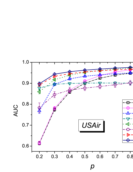
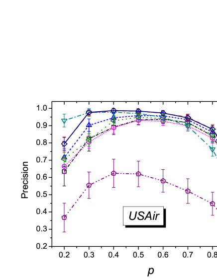
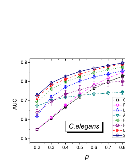
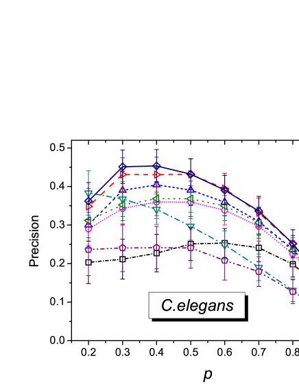
The results of these eight methods on five real networks are shown in Table 2. For each network, the training set contains 90% of the known links. Generally speaking, the global indices perform better than the local ones. And our proposed indices, LRW and SRW, can give overall better predictions than the other methods for both AUC and precision. Compared with LRW index, the SRW index can lead to an even higher accuracy. The dependence of accuracy on the proportion of training set, labeled by $p$, in USAir network and C.elegans network is shown in Fig. 1. The results indicate that the advantage of LRW index and SRW index are not sensitive to the density of the network.

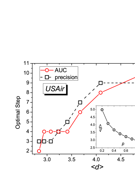
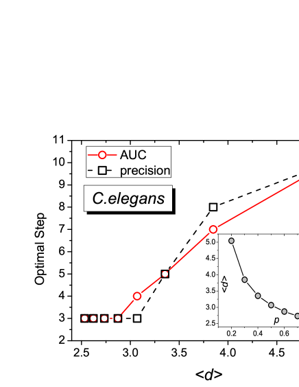
Interestingly, when predicting with the LRW index, as shown in Fig. 2, we find a positive correlation between the optimal step and the average shortest distance. For example, $\langle{d}\rangle$ of USAir and C.elegans are very small, no more than 3, their optimal steps are also small, 2 and 3 respectively in the case of $p=0.9$. However, in the power grid with $\langle{d}\rangle\approx{16}$, its AUC keeps increasing at the beginning and reaches a near optimum at step 16, where one more step leads to only 0.2% improvement. We also find that with the decreasing of $p$, the optimal step increases. This is because the removal of links to the probe set will increase $\langle{d}\rangle$, as shown in the insets of Fig. 2.

Besides high accuracy, the low computation complexity is another important concern in the design of prediction algorithm. Generally speaking, the global indices have a higher complexity than the local indices. As we known, the time complexity in calculating the inverse or pseudoinverse of an $N\times{N}$ matrix is $O(N^{3})$, while the time complexity of $n$-step LRW (or SRW) is approximately $O(N\langle k\rangle^{n})$. Science in most networks $\langle k\rangle$ is much smaller than $N$, LRW and SRW run much faster than ACT and RWR. This advantage is prominent especially in the huge-size (i.e. large $N$) and sparse (i.e. small $\langle k\rangle$) networks. For example, LRW for power grid is thousands of times faster than ACT, even when $n=10$. In HSM, the process to sample a dendrogram asks for $O(N^{2})$ steps of the Markov chain [1], and in the worse case, it takes exponential time [38]. Each step consumes a certain time to do some random selections. In addition, to predict the missing links, a large number of dendrograms are acquired. In this paper, we sample 5000 dendrograms for each implementation. Therefore, the time complexity of HSM is relatively high. It can handle networks with up to a few thousand nodes in a reasonable time, while LRW and SRW are able to handle such networks containing tens of thousands of nodes. Note that, although ACT, RWR and HSM have a higher time complexity, they provide much more information beyond link prediction. For example, the HSM algorithm can be used to uncover the hierarchical organization of real networks.

6 Conclusion

In this Letter, we proposed two similarity indices for link prediction based on local random walk, the Local Random Walk (LRW) index and the Superposed Random Walk (SRW) index. We compared our methods with six well-known methods on five real networks. The results show that our methods can give remarkably better prediction than the three local similarity indices. When comparing with the three global methods, LRW and SRW can give slightly better prediction with a lower computational complexity.