Breakdown of thermodynamic equilibrium for DNA hybridization in microarrays

Abstract

Test experiments of hybridization in DNA microarrays show systematic deviations from the equilibrium isotherms. We argue that these deviations are due to the presence of a partially hybridized long-lived state, which we include in a kinetic model. Experiments confirm the model predictions for the intensity vs. free energy behavior. The existence of slow relaxation phenomena has important consequences for the specificity of microarrays as devices for the detection of a target sequence from a complex mixture of nucleic acids.

Table 1: Target and probe sequences used in the experiments. All sequences have a 5’ to 3’ orientation. Target sequences have a 20-mer poly(A) stretch attached to their 3’ end, which terminates with a Cy3 fluorophore. Probes have a 30-mer poly(A) stretch at their 3’ end, which is covalently linked to the microarray surface.

Target sequences in solution
1.	CTTTGTCGAGCTGGTATTTGGAGAACACGT
2.	TCGAGCTGGTATTTGGAGAACACGT
Probes at the microarray surface
PM	ACGTGTTCTCCAAATACCAGCTCGACAAAG
1MM	ACGTGATCTCCAAATACCAGCTCGACAAAG
	ACGTGCTCTCCAAATACCAGCTCGACAAAG
	ACGTGGTCTCCAAATACCAGCTCGACAAAG
	…
2MM	ACGTGATCTCCCAATACCAGCTCGACAAAG
	…

DNA hybridization (the binding of two strands to form a double helix) in bulk solution has been extensively studied in the past Bloomfield et al. (2000). In this letter we discuss hybridization in DNA microarrays. Microarrays are high throughput devices which have been widely used to measure the activity of genes at a genome wide level. In a microarray singled stranded DNAs are arrayed on a solid substrate in spots, each containing a specific sequence. Hybridization takes place between surface-bound sequences (referred to as probes) and sequences in solution (targets) carrying a fluorophore. The amount of hybridized target is obtained from the emitted fluorescence from a given spot. Although hybridization in microarrays has attracted some interest in recent years its physical properties are still poorly understood (for reviews on the topic see, e.g., reviews ). We demonstrate here that, contrary to a widespread belief, in DNA microarrays equilibration times may largely exceed typical experimental times. These claims are based on experimental results and are corroborated by the analysis of a kinetic model.

The experimental setup is shown in Table 1 and extends that of Ref. Hooyberghs et al. (2009). A single sequence is present in solution: either a 30-mer or a 25-mer. The surface probe sequences are perfect matching, with one or two mismatches. The mismatches can be of different nature and they are at different positions along the sequence last_note . In total there are 1006 different probe sequences Hooyberghs et al. (2009). Custom arrays containing spots with the probe sequences of Table 1 were purchased from Agilent Technologies. We used 15K slides which accommodate 15 replicas of the 1006 sequences. The analysis is performed on the median intensities over the replicas. The standard Agilent protocol (except for target fragmentation) and Agilent buffers agi were used. The temperature is $65^{\circ}$ C.

Figure 1: Plot of $I/c$ as a function of $\Delta\Delta G$ for four different experiments at concentrations $c=2$, $10$, $50$ and $250$ pM. The hybridization time is of 17 h. The “collapse” of the four data sets into a single curve demonstrates that $I\propto c$ in the whole intensity range. Deviations from the equilibrium isotherm $I\propto e^{-\Delta G/RT}$ are observed at high intensities. Inset: plot of each individual concentration.

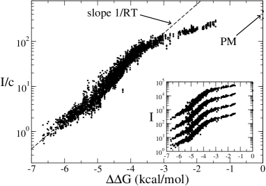
Figure 1 shows a plot of $I/c$ (the intensity divided by the target concentration) vs. $\Delta\Delta G$ for four experiments at different concentrations using the setup of Table 1 (for the 30-mer target). The variable $\Delta\Delta G\equiv\Delta G_{PM}-\Delta G$ is the difference in hybridization free energies between a given sequence and the perfect match (PM) sequence. It is calculated from the nearest-neighbor parameters obtained from the analysis of microarray data, as discussed in Ref. Hooyberghs et al. (2009) (the nearest-neighbor model assumes that $\Delta G$ can be written as a sum of dinucleotide terms Bloomfield et al. (2000)). Figure 1 shows that the intensity is proportional to the concentration for four orders of magnitude in $I$. In the low $c$ limit, equilibrium thermodynamics predicts that

$$I=Ace^{-\Delta G/RT}$$ (1)

where $A$ sets the intensity scale, $R$ is the gas constant and $T$ the temperature. Eq. (1) is obtained from the $c\to 0$ limit of the Langmuir isotherm (which was used in microarray data analysis Held et al. (2003); Naef and Magnasco (2003); Bhanot et al. (2003); Carlon and Heim (2006); Naiser et al. (2009)), but also from isotherms in which electrostatic effects are taken into account Vainrub and Pettitt (2002) (electrostatic effects were experimentally observed at low ionic strengths Gong and Levicky (2008)). In the latter $\Delta G$ contains a contribution from electrostatic interactions. For both isotherms, in the $I\propto c$ regime one expects a linear dependence of $\log I$ on $\Delta G$ (or $\Delta\Delta G$). Fig. 1 shows that the experimental data are only in partial agreement with Eq. (1), which is drawn as a dashed line in the figure.

Figure 2: Plot of intensity vs. $\Delta\Delta G$ four experiments at different times with a $30$-mer target and $c=50$ pM. Dashed lines have slope $1/RT$, dotted lines have slope $\gamma/RT$ with $\gamma=0.32$. Solid lines are obtained from the solution of Eqs. (2) and (3) using as parameters $k_{1}=10^{5}M^{-1}s^{-1}$ , $k_{2}=1s^{-1}$, $\gamma=0.32$ and $\Delta G_{\rm PM}=-14.5$ kcal/mol.

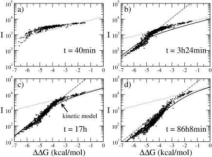
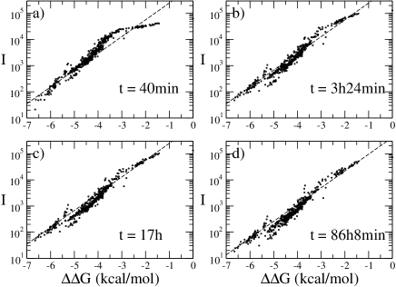
We then extended the analysis at different hybridization times. Figure 2 shows a plot of $I$ vs. $\Delta\Delta G$ for a $30$-mer target at four different times and for a concentration of $50$ pM (the $17$ h hybridization data are those already shown in Fig. 1). Once the desired hybridization time has been reached the experiment is stopped, the microarray washed and scanned to measure the emitted fluorescence from every spot. Experiments at different hybridization times thus require different slides. As the hybridization time increases, a larger fraction of the data aligns along a line with a slope $1/RT$, which shows that the observed deviations from Eq. (1) are due to the breakdown of thermodynamic equilibrium. Surprisingly, full equilibrium has not been reached here even after $86$h. In Fig. 2(b,c,d) the data for $\log I$ align along two slopes: in the equilibrium regime the slope is $1/RT$ (Eq. (1)), in the non-equilibrium regime the slope is smaller and appears to be constant in the course of time note_slope . Hybridization data for the shorter target sequence (25-mer) are shown in Fig. 3. The agreement with Eq. (1) is over three orders of magnitude in the intensity scale at times $>3$h. Hence equilibration is much faster for the shorter sequences. The experimental setup allows a detection of non-equilibrium effects as deviation from the $1/RT$ line without the need, in principle, of a time series analysis.

Figure 3: As in Fig. 2 for a target sequence of length $25$. The target concentration is $c=500$pM.

Hybridization of oligonucleotides in solution is usually described as a two state process. However, as will be shown, a two-state process cannot be reconciled with the experimental data shown in Fig. 2. During manufacturing the probes are tethered to the surface and can form a dense layer that slows down hybridization. Some of these effects have been discussed in Refs.Peterson et al. (2001); Hagan and Chakraborty (2004). The typical distance between probes is $10$ nm, and the length of a fully stretched 30-mer duplex is $10$ nm and its thickness of $2$ nm. Probe sequences in the experiment have also a poly(A) 30-mer spacer (see Table 1). Therefore a single target molecule can interact with more than one probe. Taking this into account, we have extended the two state hybridization model with an additional intermediate state (Fig. 4). Indicating with $\theta_{1}$ and $\theta_{2}$, the fraction of partially and fully hybridized probes on a microarray spot, the kinetics of these reactions is given by

$$\frac{d\theta_{1}}{dt} = ck_{1}(1-\theta_{1}-\theta_{2})+k_{-2}\theta_{2}-(k_{-1}+k_{2})\theta_{1}$$ (2)

$$\frac{d\theta_{2}}{dt} = k_{2}\theta_{1}-k_{-2}\theta_{2}$$ (3)

where $c$ is the target concentration in solution and $k_{1}$, $k_{-1}$, $k_{2}$ and $k_{-2}$ the four rates involved (see Fig. 4). For simplicity we have assumed that at most a single target molecule can bind to a given probe. $\theta_{1}$ is the average occupation fraction over several configurations in which partial binding can occur at different positions of the probe sequence.

Figure 4: The three state model for hybridization in DNA microarrays is specified by the four rate constants.

The rate constants, using a two state model description, have been measured in several microarray experiments. In Ref. Glazer et al. (2006) the hybridization of a common target sequence to a perfect match probe and to a probe containing one mismatch were considered. The following rates were measured (at $45^{\circ}$ C): $k_{1}^{\rm(PM)}=19\cdot 10^{4}M^{-1}s^{-1}$, $k_{1}^{\rm(MM)}=21\cdot 10^{4}M^{-1}s^{-1}$, $k_{-1}^{\rm(PM)}=12\cdot 10^{-4}s^{-1}$ and $k_{-1}^{\rm(MM)}=29\cdot 10^{-4}s^{-1}$. While there is more than a factor two of difference in the detachment rates, the attachment rates differ only by $10\%$. These results are in agreement with observation for kinetic behavior in bulk solution Cantor and Schimmel (1980). The probes in our experiment differ by at most two nucleotides out of 30. We will then take $k_{1}$ as sequence independent. Consider now the reaction rate $k_{2}$. In the partially hybridized state the target strand binds over a stretch of nucleotides with one probe sequence (primary contact) but it can also bind to a second neighboring probe (secondary contact). The rate limiting step is the unbinding from secondary contacts and the strand contraction so that the target probe can overcome steric hindrance and wind up into a fully formed helix all along its length. $k_{2}$ will depend on target length and probe length and density. We will assume $k_{2}$ to be the same for the probes of Table 1. The reverse rates are then fixed by the thermodynamics relations

$$k_{-1}=k_{1}e^{\Delta G^{\prime}/RT},\ \ \ \ \ \ k_{-2}=k_{2}e^{(\Delta G-\Delta G^{\prime})/RT}$$ (4)

where $\Delta G^{\prime}$ and $\Delta G$ are the free energy differences between configurations 1 and 2, and the unbound state, respectively. Next we link $\Delta G^{\prime}$ to $\Delta G$. Weak total binding (small $|\Delta G|$) caused by the presence of multiple mismatches should also correspond to weak partial binding (small $|\Delta G^{\prime}|$). As a simple approximation we will assume that the two free energies are monotonically linked as

$$\Delta G^{\prime}\approx\gamma\Delta G\ \ \ \ \ \ \ \ (\gamma<1)\,.$$ (5)

The model is thus characterized by $k_{1}$, $k_{2}$ and $\gamma$.

To gain some more insight we consider the limit of fast equilibration for Eq. (2). First we obtain the equilibrium value for $\theta_{1}$ by setting the right hand sides of Eqs. (2) and (3) to zero in the limit $ce^{-\Delta G/RT}\ll 1$. We then solve Eq. (3) replacing for $\theta_{1}$ its equilibrium value $\theta_{1}^{\rm(eq)}=ce^{-\Delta G^{\prime}/RT}$. Setting the initial condition $\theta_{2}(0)=0$ we get

$$\theta_{2}(t)=ce^{-\Delta G/RT}\left(1-e^{-t/\tau}\right),$$ (6)

$$\tau^{-1}=k_{-2}=k_{2}e^{(\Delta G-\Delta G^{\prime})/RT}=k_{2}e^{(1-\gamma)\Delta G/RT}.$$ (7)

The relaxation time, $\tau$, depends on $\Delta G$: weakly bounded sequences (small $|\Delta G|$) equilibrate faster than strongly bounded ones (large $|\Delta G|$). For fast equilibrating sequences ($\tau\ll t$) one recovers Eq. (1) from Eq. (6); for sequences with long equilibration times $\tau\gg t$ we expand Eq. (6) to lowest order in $t/\tau$. With this approximation we find that for a given time $t$

$$\theta_{2}(t)=\left\{\begin{array}[]{ccc}ce^{-\Delta G/RT}&&|\Delta G|\ll|\Delta G^{*}|\\ ctk_{2}e^{-\gamma\Delta G/RT}&&|\Delta G|\gg|\Delta G^{*}|\end{array}\right.$$ (10)

where $\Delta G^{*}$ is a crossover free energy that depends on time and is obtained by setting $\tau=t$ in Eq. (7). After hybridization the slides undergo washing steps according to the standard Agilent protocol, which are expected to remove weakly bound target molecules from the slide and have been also included in thermodynamics models of arrays wash . In the present setup there is only one target sequence in solution and washing is likely to affect the partial hybridized state. In this case one can assume that the measured intensity is given by $I\approx A\theta_{2}$ (in the model the typical free energies of the partially hybridized states are such that $\theta_{1}\ll\theta_{2}$). Equation (10) reproduces the two slopes in the $\log I$ vs. $\Delta\Delta G$ plots as seen in the experiments (Fig. 1). It shows that the non-equilibrium regime is characterized by a slope equal to $\gamma/RT$.

The solid lines in Fig. 2(b,c,d) are plots of the intensity $I=A\theta_{2}$ obtained from the solution of Eqs. (2) and (3). The parameters used are given in the caption of Fig. 2. For the choice of parameters given, the fast equilibration limit (Eq.(6)) approximates very well the full solution of Eqs. (2) and (3). There is a reasonable agreement between the experiments and the kinetic model. We note though that the crossover between the two regimes is somewhat sharper in experiments. In addition, the experimental $I$ vs. $\Delta\Delta G$ data show a slight sigmoidal trend which is not present in the kinetic model. Within the two state model kinetics, and using the assumption $k_{1}$ as sequence independent, one arrives to a solution similar to Eq. (10) although with $\gamma=0$. Therefore the two state model cannot account for a second finite slope as observed in the experiments. Note that the fit of the kinetic model to the data requires also an estimate of $\Delta G_{\rm PM}$, as the method of Ref. Hooyberghs et al. (2009) does not provide absolute $\Delta G$ for a sequence but only $\Delta\Delta G$, i.e. differences in free energies with respect to a perfect match hybridization. In addition, in the fit we adjusted the constant $A$ ($I=A\theta_{2}$) as we note in the experimental data a global decrease of the intensity scale. This is probably due to some degradation of the fluorophores or of the target and probe strands (as depurination, the loss of purines, which alters the binding energies of the involved strands). The overall decrese in intensity occurs both for the 25-mer and the 30-mer sequences. In the latter the effect is somewhat stronger, especially at longer hybridization times.

Eq. (7) predicts that the relaxation time is a function of $\Delta G$, $\Delta G^{\prime}$ and $k_{2}$. We can use this equation to compare the ratio between the times for a $L=30$ and $L=25$ targets. Consider the same probe sequence hybridizing to the two targets. Assuming $\Delta G^{\prime}(L=30)\approx\Delta G^{\prime}(L=25)$ and using as estimate of the difference in binding energies between $\Delta G(L=30)-\Delta G(L=25)\approx-2.5$ kcal/mol note1 , we get from Eq. (7) a decrease of a factor $\exp(2.5/RT)\approx 40$ in the relaxation time. In addition one also expects $k_{2}(L=25)>k_{2}(L=30)$ which decreases the relaxation time even further. The similarities between Fig. 2(c) and Fig. 3(a) suggest that the relaxation time ratio between $25$-mers and $30$-mers is approximately $25$, which is the same order of magnitude just obtained from Eq. (7). Since typical biological experiments involve target strands of lengths 30-50, the breakdown of equilibrium shown here may occur in many different microarrays platforms and in biological experiments, and could involve even longer relaxation times.

Summarizing: We showed that hybridization in DNA microarrays under standard conditions is characterized by relaxation times which may largely exceed the experimental time. In the non equilibrium regime the intensities are distributed as $e^{-\gamma\Delta G/RT}$, with $\gamma<1$. This is equivalent to introducing an effective temperature $T_{\rm eff}=T/\gamma>T$. Interestingly effective temperatures were used as adjustable phenomenological parameters to fit biological microarray data Held et al. (2003); Carlon and Heim (2006). This work provides an insight on the origin of these.

The breakdown of equilibrium implies lower specificity of the microarrays as devices for the detection of a desired sequence from a complex mixture. To see this consider a probe at the microarray surface and two sequences at equal concentration in solution: one perfect matching with the probe and one with a mismatch. In the equilibrium regime the two sequences hybridize to the probe with a probability ratio $e^{(\Delta G_{PM}-\Delta G_{MM})/RT}\approx 0.05$, where we have used a typical value $\Delta G_{MM}-\Delta G_{PM}\approx 2$ kcal/mol Hooyberghs et al. (2009) and a temperature of $T=65^{\circ}$ C. In the nonequilibrium regime, due to the presence of a factor $\gamma<1$ in the exponential the ratio is about $0.4$ (taking $\gamma=0.32$). Therefore in the non-equilibrium regime a significant fraction of a measured signal may be due to hybridization to non-complementary targets, a phenomenon known as cross-hybridization. For an optimal functioning of the microarrays it is then desirable to work under equilibrium conditions Bhanot et al. (2003). Several parameters may influence the relaxation time as temperature, salt and buffer conditions. The experimental setup discussed in this paper provides a good test of equilibrium (single line vs. broken line in a $I$ vs. $\Delta\Delta G$ plot) and can be used to investigate the best working conditions for hybridization.